

Abstract
Objective. The correspondence between the anatomical STN and the STN observed in T2-weighted MRI images used for deep brain stimulation (DBS) targeting remains unclear. Using a new method, we compared the STN borders seen on MRI images with those estimated by intraoperative microelectrode recordings (MER). Approach. We developed a method to automatically generate a detailed estimation of STN shape and the location of its borders, based on multiple-channel MER measurements. In 33 STNs of 19 Parkinson patients, we quantitatively compared the dorsal and lateral borders of this MER-based STN model with the STN borders visualized by 1.5 T (n = 14), 3.0 T (n = 10) and 7.0 T (n = 9) T2-weighted MRI. Main results. The dorsal border was identified more dorsally on coronal T2 MRI than by the MER-based STN model, with a significant difference in the 3.0 T (range 0.97–1.19 mm) and 7.0 T (range 1.23–1.25 mm) groups. The lateral border was significantly more medial on 1.5 T (mean: 1.97 mm) and 3.0 T (mean: 2.49 mm) MRI than in the MER-based STN; a difference that was not found in the 7.0 T group. Significance. The STN extends further in the dorsal direction on coronal T2 MRI images than is measured by MER. Increasing MRI field strength to 3.0 T or 7.0 T yields similar discrepancies between MER and MRI at the dorsal STN border. In contrast, increasing MRI field strength to 7.0 T may be useful for identification of the lateral STN border and thereby improve DBS targeting.
Export citation and abstract BibTeX RIS
Corrections were made to this article on 18 October 2016. A spelling was corrected in the title and the first line of the abstract.
1. Introduction
Deep brain stimulation (DBS) of the subthalamic nucleus (STN) is an effective surgical treatment to alleviate the symptoms of severe Parkinson's disease (PD) [1–4]. The surgical procedure [5], as well as the stimulation itself may lead to side effects [6–9]. These include side effects like tonic motor contractions and rhythmic myoclonus in the face [7], paraesthesia, dysarthria [6] and effects on cognition and mood [8, 9]. Stimulation-induced side effects are attributed to the aberrant stimulation of the limbic and associative subareas of the STN or structures outside the STN and are therefore dependent on the location of the stimulating contact [10–13]. Therapeutic effects of STN-DBS can be improved and stimulation-induced side effects can be avoided by specifically targeting the dorsolateral portion of the STN [14–18], which is associated with sensorimotor function [13, 19, 20]. Therefore, it is essential that localization of the STN is performed as accurately as possible.
Targeting of the STN for the implantation of DBS electrodes has shifted from an indirect approach to direct visualization of the STN. In the indirect approach, autopsy-based atlases were used to provide the coordinates of the STN relative to landmarks that were established with imaging techniques that do not show the STN itself [21–24]. With the advances in MRI, it became possible to directly visualize (parts of) the STN on preoperative images and establish a stereotactic target for the STN directly based on the hypointense signal observed on T2-weighted MRI images [21, 24–28]. This patient-specific approach is based on the contrast between white and gray matter by which the contours of the STN can be identified in the MRI images [24, 29]. However, disadvantages of this direct visualization are its dependence on high-quality images and the fact that different forms of MRI sequencing result in different STN shapes and sizes [12, 24, 29–31]. For these reasons, the correspondence between the STN observed in T2-weighted MRI images and the exact anatomical STN still remains unclear [32]. High field strength T2 MRI can improve visualization of the STN and it could therefore possibly improve the direct targeting approach [33–37].
For additional verification of the STN position after imaging, microelectrode recordings (MER) are often performed during DBS surgery to delineate the boundaries of the STN [21, 30, 38]. The interpretation of high frequency spiking activity measured with MER thereby helps to guide electrode placement and allows the neurosurgeon to adjust MRI-based targeting [39, 40]. The primary purpose of intraoperative MER measurements is to define the dorsal and ventral borders of the STN along each planned electrode path and to identify the most lateral path that passes through the STN with sufficient length [41]. Additionally, the differences between the STN dimensions based on MRI contrast and the STN dimensions based on intraoperative MER measurements could be evaluated postoperatively [32].
The discrepancies between T2 MRI and MER in STN targeting have been the subject of several studies [21, 30, 32, 40, 42–45]. Most studies discuss the additional value of MER by reporting how frequently extra MER channels need to be added to the central one when the recordings demonstrated that MRI targeting was insufficient [43, 44]. Some studies report on how the use of MER alters the predefined MRI target for DBS implantation [21, 36, 40, 42, 45]. Only a few studies actually perform a direct comparison between the STN borders estimated by preoperative T2 MRI and those found by MER [30, 32]. Hamani et al concluded that the STN was underestimated on 1.5 T T2 MRI images and mainly extended more anteriorly than was determined by T2 MRI [30]. Polanski et al reported a relatively low positive predictive value (65.5%) of 3.0 T T2 MRI for the MER-based STN and a high negative predictive value (82.5%), indicating that the STN was estimated larger on T2 MRI than it was by MER [32]. Overall, literature suggests that the borders of the STN are variable between patients and comparisons between MER and T2 MRI in literature are not always able to point out exactly where the discrepancies lie and are even sometimes contradictory [12, 30, 32, 42].
In the present study, a method was developed to automatically generate a detailed STN model that includes estimation of STN size, shape, and the location of its borders, based on the classifications of multiple-channel MER measurements. This estimated MER-based STN model can be easily fused with all available preoperative images and then a detailed one-on-one comparison can be performed between the STN borders seen in the MRI images and those estimated based on the MER measurements without the need for changes in standard surgical procedures. The goal of this study was to quantify the discrepancies between MRI and MER at the borders of the STN. We have compared these discrepancies between MRI images made with low (1.5 T), high (3.0 T) and ultra-high (7.0 T) magnetic field strengths.
2. Methods
This study consists of two separate phases. In the first phase, the model building algorithm was optimized by determining the correct boundaries for MER-based STN estimation. For this, a large dataset of preoperative images and MER measurements was used. In the second phase, the STN models created by the algorithm were used to quantitatively compare the MRI-based STN with the MER-based STN. For this second phase, a second dataset was used to prevent overfitting of the models to the initial dataset.
2.1. Surgical procedures and MER measurements
All patients presented in this study underwent DBS using either a one-stage bilateral or unilateral stereotactic approach, including MERs and test stimulation. STN target calculation and path planning was done with frame-based T2 MRI using the Leksell stereotactic frame and Surgiplan software (Elekta Instruments AB, Stockholm, Sweden). Standard STN coordinates (11–12 mm lateral, 2 mm posterior, and 4 mm ventral to the midcommissural point) were visually adjusted by the neurosurgeon if necessary. Cerebrospinal fluid (CSF) loss and subdural air invasion was minimized by planning the paths to enter on top of a precoronal gyrus, by operating patients while in a semi-sitting position with the head elevated at 20°–30° and by closing the burr holes with fibrin glue after introduction of the microelectrodes [46].
To identify the STN during surgery, MER measurements were performed with one to five steel cannulas and microelectrodes (FHC, Inc., Bowdoin, ME, USA). The MER electrodes were arranged in a cross-shaped array with an inter-electrode distance of 2 mm. MER measurements started 6 mm above the planned STN target, simultaneously advancing downward in 0.5 mm steps until substantia nigra activity was visible in at least one channel or STN activity significantly decreased in all channels.
Over time, two different systems were used for the MER measurements; first the Leadpoint system (Medtronic, Minneapolis, MN, USA) and later the ISIS MER System (Inomed, Emmendingen, Germany). Using the Leadpoint system, recordings were amplified with a gain of 10 000, analogue bandpass filtered between 500 Hz and 5000 Hz and sampled at 12 kHz. Later, using the ISIS MER System, recordings were amplified with a gain of 10 000, analogue bandpass filtered between 160 Hz and 5000 Hz and sampled at 20 kHz. Although the two recording techniques are slightly different, this should not interfere with the identification of STN activity. Both systems are well able to measure single/multi-unit spiking within 100–200 μm of the electrode [47] and overall background activity. Recordings were visually assessed by an experienced physicist and a neurologist who scored them as recorded either inside or outside the STN. The scoring of MER measurements was based on the observed abrupt increase in background activity upon entry into the STN combined with the amount of single/multi-unit spiking activity [39, 41, 48].
2.2. Phase 1: optimization of the model building algorithm
In the first phase, to optimize the model building algorithm, we studied the surgical records and MRI images of 34 PD patients (63 STNs) who underwent DBS surgery in the Academic Medical Center in Amsterdam between April 2004 and July 2007.
To estimate patient-specific models of STN size and position, the model building algorithm used the classifications of MER measurements, either inside or outside the STN, to fit an atlas-derived representation of the STN onto the coordinates of the MER sites. The MER coordinates were all in reference to the stereotactic frame, which is recognized in the Surgiplan software that is used for preoperative targeting. Only MER tracks that passed through the STN were used in the model building algorithm [49, 50]. Tracks that did not show STN activity in any of its recordings were excluded. This was done because high values of electrode impedance and other possible microelectrode malfunctioning could have interfered with the visual MER assessment and it could therefore not be concluded with certainty that these tracks missed the STN, which could induce large estimation errors in the model.
STN fitting was performed off-line using MATLAB (Mathworks, Inc., Natick, MA, USA). The original STN representation was a three-dimensional polygon surface extracted from the Cicerone software package [51, 52]. First, this STN body was placed with its center on the planned stereotactic target, then both the STN body and the MER sites were rotated using the arc and ring angles of the preoperative planning, such that the MER trajectories were aligned parallel to the z-axis. This MER-based orientation, centered on the planned stereotactic target, is the starting point of the optimization procedure. This was done so to be able to estimate appropriate boundaries for the STN fitting algorithm based on the directions in which there was either a high or low density of MER measurements. From here, the size and location of the patient-specific STN was estimated based on the MER classifications. Using an optimization routine, the initial 3D body was translated, rotated and scaled in all three directions (in total nine degrees of freedom) to fit the classifications of the MER sites as good as possible. The optimization routine itself has been described in more detail by Lourens et al [49] initial boundaries for the transformations were based on the variability of STN size and location reported by Daniluk et al [12] and were ±2 mm translation in all directions, ±20° rotation around all axes and ±25% scaling in all directions. To obtain the best possible estimation of STN size and location, the optimization routine was performed 50 times. The best fittings were selected by excluding all STNs for which the fitting value, which was minimized in the optimization routine, exceeded the median fitting value of 50 iterations. From the remaining STNs, the model that had the lowest amount of total transformation was chosen as the best STN model.
The model building algorithm was further optimized by examining the size and location of MER-based STN models in relation to the preoperative 1.5 T T2 MRI images and determining the appropriate boundaries for the transformations. For this, cross-sections of the best STN model in stereotactic orientation were made at 0.5 mm slices with a pixel size of 0.5 mm × 0.5 mm. The contours of these cross-sections were then exported as a set of DICOM images. Every DICOM image included markers on the stereotactic coordinates of the Leksell frame fiducials. This created an image of the same stereotactic frame as the one used in preoperative targeting, together with a patient specific STN body which is in reference to this frame. The images were then imported into the Surgiplan software with the original frame recognition and co-registered to the preoperative images using the stereotactic frame. The overlays of MER-based STN contours and the T2 MRI images of the STN were then independently evaluated in axial and coronal images by two experienced DBS neurosurgeons (P.R.S. and P.v.d.M.). Cases with too much rotation, translation or scaling were identified based on the discrepancies between the contours of the STN model and parts of the STN border that were well visible on 1.5 T T2 MRI. Based on these cases, realistic boundaries for all transformations were identified in relation to the information available for the optimization routine, that is, the amount of MER trajectories that measured STN activity. Visual assessment of the fused images suggested that at least three MER tracks were needed for adequate estimation of the STN; this was not the case in 8 out of 63 STNs. The specific transformation boundaries for STNs estimated by three or more tracks can be found in the supplementary materials (table S1). In general, the presence of more MER trajectories passing through the STN results in more freedom for the optimization routine to transform the STN. If a certain direction of the cross-shaped array only has two MER tracks instead of three, then the freedom for transformations in this direction was limited. Transformations affecting the dorsoventral dimensions of the STN had the highest degree of freedom and were independent of the number of MER tracks available. This was done because the resolution of MER classifications is highest in this direction and therefore these transformations will always be accurately limited.
2.3. Phase 2: quantified comparison between the MER-based STN model and the MRI-based STN
In the second phase of this study, after optimization of the model building algorithm, a new dataset was used to compare the STN borders in a quantitative manner. The first phase of model optimization suggested that at least three MER tracks were needed for adequate estimation of the STN, therefore in the second dataset only STNs for which three or more MER tracks showed STN activity were included. Additionally, cases in which only three MER tracks showed STN activity were not included when these three tracks were in the same plane (e.g., when only the lateral, central and medial channels in the cross-shaped array showed STN activity). This new dataset was composed out of the surgical records and T2 MRI images of PD patients who underwent DBS surgery in the Academic Medical Center in Amsterdam between November 2009 and November 2015. Surgical procedures were identical to those in the first dataset. From this period, three groups of patients were selected based on the field strengths in which T2-weighted MRI images were available: 1.5 T, 3.0 T or 7.0 T. The MRI images that were used for the quantitative comparison were the same as the images used for preoperative targeting. A strict selection of patients was performed to ensure that only MRI images of the highest possible quality were used for STN identification in all groups. Figure 1 shows examples of both axial and coronal cross-sections of the STN in T2-weighted MRI images in the three different groups.

Figure 1. Examples of STN imaging using T2-weighted MRI in three different field strengths. Figures (a)–(c) show axial cross-sections of the STN in 1.5 T, 3.0 T and 7.0 T MRI respectively. Figures (d)–(f) show coronal cross-sections of the STN in 1.5 T, 3.0 T and 7.0 T MRI respectively.
Download figure:
Standard image High-resolution imageTo objectively compare the STN borders on these MRI images with the MER-based STN borders, one neurosurgeon (P.R.S.) used the coronal MRI images to identify the borders without knowledge of the MER-based STN borders. The STN identification was performed in the Surgiplan software with the original stereotactic frame recognition, The neurosurgeon that performed the anatomical STN identification had extensive experience with this software and with STN identification in 1.5 T, 3.0 T and 7.0 T MRI images. If however, he was unable to accurately identify the STN borders in a certain patient because of low quality MRI images, this patient was excluded from further analysis. This resulted in 19 PD patients that were used for the quantitative analysis. Table 1 shows the number of patients and STNs included in each group together with the MRI systems, MRI sequences and specific scanning parameters that were used to obtain images of the STNs. While in the 1.5 T and 3.0 T groups we used coronal MRI images with a good in-plane resolution and a slice thickness of 2 mm, in the 7.0 T group the in-plane coronal MRI images often suffered from motion artifacts and we had to use the coronal reconstruction of the 3D T2 acquisition instead.
Table 1. Overview of the number of patients and STNs included and the scanning parameters used to obtain MRI images of the STNs in the three groups of different magnetic field strengths.
| Field strength | MRI system | MRI sequence | TR (ms) | TE (ms) | Voxel size [x, y, z] (mm × mm × mm) | Number of patients | Number of STNs 7 |
|---|---|---|---|---|---|---|---|
| 1.5 T | Siemens Avanto5 | Coronal T2-weighted TSE | 5750 | 99 | 0.5 × 2.0 × 0.5 | 8 | 14 |
| 3.0 T | Philips Ingenia6 | Coronal T2-weighted TSE | 4823 | 80 | 0.4 × 2.0 × 0.4 | 5 | 10 |
| 7.0 T | Philips Achieva6 | Three-dimensional T2-weighted TSE | 3000 | 295 | 0.7 × 0.7 × 0.7 | 6 | 9 |
5Siemens Healthcare, Erlangen, Germany. 6Philips Healthcare, Eindhoven, The Netherlands. 7In the 1.5 T group, only 14 out of 16 imaged STNs were used because in 2 STNs less than three MER tracks were available. In the 7.0 T group, only 9 out of 12 imaged STNs were used because of the same reason. TE = echo time, TR = repetition time, TSE = turbo spin-echo.
All T2 MRI images were co-registered with the 1.5 T axial T1 images with stereotactic frame and MRI-based STN borders were identified based on the difference in contrast between the gray matter of the STN and the surrounding white matter. The initial visual comparison, performed during the optimization of the model building algorithm, showed the greatest discrepancies between MER-based and MRI-based STN at the dorsal and lateral borders. Moreover, the dorsolateral part of the STN is associated with sensorimotor function, which makes the dorsal and lateral borders the most relevant borders to identify. Therefore, the quantitative comparison focused on both these borders, but especially on the dorsal border because the accuracy of the MER-based STN estimation was highest in the dorsoventral direction.
Three coronal T2 MRI images were used to identify six points that represent the dorsal and lateral STN borders. MRI-based borders were identified in a coronal image based on the y-coordinate of the target. Three points were placed by the neurosurgeon representing the dorsal border in this image on (1) the most lateral part of the dorsal border visible on the MRI, (2) on the dorsal border 2 mm more medial than the first point and (3) on the dorsal border 2 mm more medial than the second point (points 1–3, figure 2(b)). Two more points were identified on the most lateral part of the dorsal border in the coronal images which were 2 mm more anterior (point 4, figure 2(c)) and 2 mm more posterior (point 5, figure 2(a)) to the central image. Finally, a 6th point was placed on the most lateral part of the STN in the central image, approximately 3 mm ventral to the dorsal border (point 6, figure 2(b)).
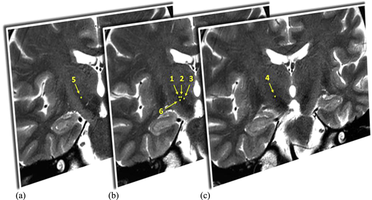
Figure 2. Example of three coronal 3.0 T T2-weighted MRI images, (b) the central image closest to the y-coordinate of the stereotactic target on the right side, (a) the image 2 mm more posterior and (c) 2 mm more anterior. In these images the dorsal (1–5) and lateral (6) border points of the right STN are identified by the neurosurgeon.
Download figure:
Standard image High-resolution imageThis procedure resulted in six points representing the most relevant STN borders in reference to the original stereotactic frame that was used for preoperative targeting and thus for the creation of the MER-based STN model. These six stereotactic coordinates were then exported from the Surgiplan software to MATLAB. There, the MER-based STN model was combined with the points that represent the MRI-based STN borders, both in reference to the original stereotactic frame. An example of this is shown in figure 3. Both the STN model and the identified border points were rotated from the patient specific stereotactic orientation to the general AC-PC aligned orientation. In this orientation, the dorsoventral distances between the dorsal border points (points 1–5) and the dorsal border of the MER-based STN model directly above or beneath it were calculated. Additionally, we calculated the mediolateral distance between the lateral border point (point 6) and the lateral border of the STN model directly medial or lateral to this point.
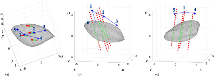
Figure 3. Example of the model STN body (gray) fitted onto the classifications of the MER sites (red dot = outside, green dot = inside) viewed from a (a) dorsal, (b) anterior and (c) lateral perspective. The blue crosses represent the STN dorsal and lateral border points as they are identified in coronal 1.5 T, T2-weighted MRI images. In every view, only the most relevant border points for that perspective are displayed. The numbering on the axes shows the distance to the stereotactic target in mm. (For interpretation of the references to color in this figure legend, the reader is referred to the web version of this article.)
Download figure:
Standard image High-resolution image2.4. Statistical analysis
Two-way ANOVA was used to compare mean values of size and location of the MER-based STN models between the three groups; the 1.5 T, 3.0 T and 7.0 T MRI groups. Similarly, the mean amount of transformation in all directions was compared between groups.
The quantified difference between the MRI-based STN border points and the MER-based STN borders was compared to a value of zero using two-tailed one-sample t-tests with Bonferroni correction (n = 6). This was done for all three groups of images independently.
3. Results
3.1. Patient data
For the comparison between the MER-based STN and the MRI-based STN, the MER records and MRI images of 33 STNs in 19 patients were examined. The clinical characteristics of the patients are shown in table 2. In eight patients, 14 STNs were compared using 1.5 T MRI images, in five patients, 10 STNs were compared using 3.0 T MRI images and in six patients, 9 STNs were compared using 7.0 T MRI images. Two-way ANOVA showed no significant differences in clinical characteristics between the 1.5 T, 3.0 T and 7.0 T groups.
Table 2. Clinical characteristics of the 19 patients at time of surgery (mean ± SD, [range]).
| Patient characteristics | Values (n = 19) |
|---|---|
| Male/female | 10/9 |
| Age (years) | 61.1 ± 6.0, [48.6–70.5] |
| Disease duration (years) | 12.6 ± 5.0, [7.4–29.4] |
| UPDRS part III motor score OFF medication | 44.4 ± 12.3, [31–77] |
| UPDRS part III motor score ON medication | 20.0 ± 6.5, [8–34] |
UPDRS = Unified Parkinson's disease rating scale.
3.2. MER-based STN models
Using the optimized STN fitting routine, 33 MER-based STN models were created. Characteristics describing the size and location of these STN models are shown in table 3. Statistical testing of the variables in table 3 with two-way ANOVA showed no significant differences in MER-based STN size and location between the 1.5 T, 3.0 T and 7.0 T groups. Additionally, no significant differences between the three groups were found when comparing the amount of transformation. This was found for all transformations (translation, rotation and scaling) in all individual directions (x, y and z).
Table 3. Characteristics (mean ± SD, [range]) describing the size and location of the 33 MER-based STN models in an AC-PC aligned orientation.
| STN characteristics8 | Values (n = 33) |
|---|---|
| Dorsoventral dimension (mm) | 5.3 ± 0.5, [4.5–7.3] |
| Anteroposterior dimension (mm) | 8.2 ± 0.5, [7.2–9.2] |
| Mediolateral dimension (mm) | 9.1 ± 0.9, [7.4–11.0] |
| Target x-coordinate (mm lateral to MCP) | 11.0 ± 0.8, [8.4–12.2] |
| Target y-coordinate (mm posterior to MCP) | 2.4 ± 0.5, [1.4–3.9] |
| Target z-coordinate (mm ventral to MCP) | 4.1 ± 0.4, [3.4–5.4] |
8All measures of size and location were assessed in an AC-PC aligned orientation. The STN dimensions were assessed by calculating the difference between two most extreme points in a certain direction. MCP = midcommissural point.
3.3. Quantified comparison between MER-based STN and MRI-based STN
The results of the assessment of dorsoventral distances between the five dorsal border points identified in the MRI by the neurosurgeon and the dorsal borders of the MER-based STN models are shown in figure 4. Per group, for each of the dorsal border points, the mean distance in millimeter plus and minus one standard deviation of the distribution is shown. Here, a positive distance indicates that the dorsal border of the STN was identified more dorsally on MRI than it was by MER. In figure 4(a), the comparisons of points 1, 2 and 3 in the MRI are shown against a centrally located coronal cross-section of the MER-based STN model. Figure 4(b) shows the comparisons of points 1, 4 and 5 in the MRI against a sagittal cross-section of the MER-based STN.

Figure 4. Overview of discrepancies between MRI-based STN and MER-based STN at the dorsal border. Shown are the mean distances in millimeters plus and minus one standard deviation, a positive distance indicates that the dorsal border of the STN is identified more dorsally by MRI than it is by MER. Results significantly different from zero are marked. (a) Comparisons of (from left to right) points 1, 2 and 3 identified in the MRI. For comparison with the MER-based STN, a centrally located coronal cross-section the STN model is shown. (b) Comparisons of (from left to right) points 5, 1 and 4 identified in the MRI. For comparison with the MER-based STN, a laterally located sagittal cross-section the STN model is shown.
Download figure:
Standard image High-resolution imageThe average identification of the dorsal border of the STN based on the MRI was located more dorsally on all points compared to the MER-based STN. Two-tailed one-sample t-tests with Bonferroni correction (n = 6) showed that, in the 3.0 T and 7.0 T groups, the lateral part of the dorsal border was identified significantly more dorsal on the MRI than by the MER-based STN model (i.e., the distance was significantly greater than zero). In the 3.0 T group, significant differences were found at the lateral part of the dorsal border at the central (point 1, M = 0.97 mm, p < 0.001), anterior (point 4, M = 1.05 mm, p = 0.006) and posterior (point 5, M = 1.19 mm, p = 0.002) levels. The 7.0 T group, shows significant differences at the central (point 1, M = 1.23 mm, p < 0.001) and anterior (point 4, M = 1.25 mm, p = 0.002) levels of the dorsolateral border.
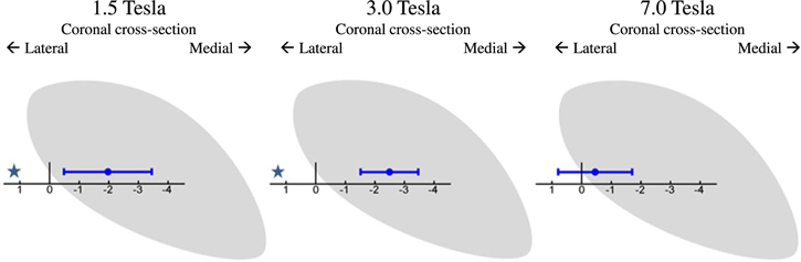
Figure 5 shows the results when comparing the lateral border point identified on the MRI with the lateral border of the MER-based STN model for the three groups. Here, a negative distance indicates that the lateral border was identified more medially by MRI than it was by MER. Two-tailed one-sample t-tests with Bonferroni correction (n = 6) showed that the lateral border was identified significantly more medial on the MRI (i.e. the distance was significantly smaller than zero) in both the 1.5 T (point 6, M = −1.97 mm, p < 0.001) and 3.0 T (point 6, M = −2.49 mm, p < 0.001) group.
Figure 5. Overview of discrepancies between MRI-based STN and MER-based STN at the lateral border. Shown are the mean distances in millimeters plus and minus one standard deviation, a negative distance indicates that the lateral border of the STN is identified more medially by MRI than it is by MER. Results significantly different from zero are marked. For comparison with the MER-based STN, a centrally located coronal cross-section the STN model is shown.
Download figure:
Standard image High-resolution image
4. Discussion
The results of this study suggest that there are discrepancies between the borders of the STN identified by MRI and those identified by MER, found at the dorsal border and at the lateral border. These discrepancies are different depending on the field strength of the T2 MRI used for identification of the borders.
4.1. Discrepancies at the dorsal STN border
Both the 3.0 T group and the 7.0 T group showed significant differences at the lateral part of the dorsal border. The mean difference was comparable between the two groups and indicates that the dorsal border was identified approximately 1.00–1.25 mm more dorsally by MRI than by MER. The mean difference in the 1.5 T group was similar, but it did not reach significance because of the larger spread of observations. This spread decreases with the increase in field strength from 1.5 to 3.0 T which can be explained by the increased signal to noise ratio and increased MRI contrast obtained with higher field strengths. Furthermore, the voxel size decreases from 0.5 × 2.0 × 0.5 mm3 to 0.4 × 2.0 × 0.4 mm3. This leads to an MRI image with a higher spatial resolution and better MRI contrast and should therefore lead to a more precise identification of the STN border. However, only the spread of the observations seems to decrease, while the mean difference between the MRI-based border and the MER-based border remains the same. Even when field strength increases to 7.0 T, a mean difference remains. This may indicate that the discrepancies at the dorsal border are not just the result of a random error due to low MRI contrast, but also of a systematic difference in the visualization of the STN on MRI and the localization of the STN based on MER. This systematic difference implies that either there is a systematic error in the used comparison method or the dorsal border of the STN as seen on MRI extends beyond the functional border as found by MER.
Errors in the comparison itself can be caused by inaccuracy of the co-registration of T1 and T2 images or by inaccuracies in the stereotactic frame [53]. However, these errors would be random errors and can explain some of the variance, but they cannot explain the systematic difference. A systematic difference might by caused by the comparison of the preoperative brain (on MRI) with the intraoperative brain (on MER) due to either positional differences of the brain or brain shift caused by CSF leakage. However, it is very unlikely that brain shift caused by leakage of CSF is the cause as CSF leakage is kept to an absolute minimum by the surgical procedures described in the methods [46, 54] and CSF leakage would mainly lead to posterior displacement of the frontal lobe with very little effect on the basal structures like the STN [55, 56]. Because of the different effect of gravity when comparing preoperative MRI taken in supine position, with intraoperative MER taken in semi-sitting position, a caudal displacement of the brain could possibly be a contributing cause of the difference found in this study. Another contributing factor to the more ventral location of the STN as determined by MER could be that the insertion of several cannulas for the MER close to the STN actually causes drag and compression, resulting in a ventral displacement of the structures during surgery. Misidentification of the STN on MER measurements is unlikely to be the cause of the systematic difference. The STN is very densely populated with neurons and, therefore, the observed increase in background activity is easy to identify and abrupt [41]. A structural border zone that does not display typical neuronal firing has not been reported. Although the density of MER measurements around the dorsal STN border is high, the distance between two successive measurements in the same trajectory is still 0.5 mm. This will result in an imprecision in MER-based dorsal border estimation of maximally 0.5 mm. Moreover, the model building algorithm will interpolate the border somewhere between a MER site classified as inside the STN and one classified as outside the STN. This interpolation is also based on the information from surrounding MER trajectories, which will likely make the imprecision less than 0.5 mm. Again, this imprecision would lead to a random error and could explain some of the variance observed in the discrepancies at the dorsal border, but it cannot explain the systematic difference that has been observed.
A plausible explanation for the systematic difference is that the dorsal anatomical border of the STN seen on MRI extends beyond the functional border found by MER. The systematic difference we found on the anterior side of the dorsolateral border of STN might be associated with the findings of others that the anteriorly located pallidofugal fiber pathways result in extra hypointense T2 MRI signal and are therefore difficult to distinguish from the STN [26, 30]. Previous reports on discrepancies between MER and T2 MRI have been contradictory [30, 32]. While Hamani et al [30] showed a smaller estimation of the STN in the dorsoventral direction on T2 MRI compared to MER, Polanksi et al [32] showed a larger estimation on T2 MRI. The contradicting results at the dorsal border in previous studies could be the result of a limited analysis of the locations of MER measurements. MER trajectories are often analyzed separately or the location of the MER sites with respect to the STN is only based on the preoperative planning. The advantage of this study lies in the detailed estimation of the complete STN based by multiple channel MER measurements. Thereby, we could locate the discrepancies between MER and MRI more accurately and discriminate between discrepancies at the anterior and posterior levels of the dorsal border. This can be seen in figure 4(b) in the sagittal cross-section of the 7.0 T results. A significant difference of approximately 1.25 mm was found at the central and anterior level of the dorsolateral border, possibly the result of extra hypointense T2 MRI signal caused by the pallidofugal pathways, while at the posterior level of the dorsolateral border, a large variability but no mean difference was found, which may possibly be caused by the smaller iron content and consequently a less accurate delineation of the posterior STN by hypointense T2 MRI signal [26].
4.2. Discrepancies at the lateral STN border
Figure 5 shows that in the 1.5 T and the 3.0 T groups the lateral border was identified significantly more medial on coronal T2 MRI images than by MER. The mean differences found in these groups are approximately 2.0–2.5 mm. Similarly to the dorsal border, the spread decreases with increased field strength from 1.5 to 3.0 T. Again, this may be caused by the increase in MRI contrast and the decrease in voxel size which should lead to a more precise identification of the lateral border. However, a significant discrepancy between MRI and MER still remains. When the field strength increases further to 7.0 T, the mean difference between the lateral border on MRI and the border estimated by MER greatly decreases and was no longer significantly different from zero. This may indicate that the observed mismatch in the 1.5 T group, and even in the 3.0 T group, might be the result of insufficient T2 MRI contrast on coronal images at the lateral border which makes it difficult to discriminate the lateral part of the STN from the adjacent internal capsule. This finding is different from the study by Hamani et al [30] in which no STN activity was found outside the lateral border of the STN identified on 1.5 T T2 MRI images. Again, the more detailed estimation of the STN in our study may explain this difference. Fitting a 3D body of the nucleus onto the MER sites, can lead to an estimation of the lateral border several millimeters past the most lateral MER trajectory. For example, the combination of a relatively short trajectory with STN activity on the central channel with a very long trajectory on the lateral channel implies that the STN will extent some more laterally where there were no MER measurements. This estimation, compared to the limited identification of the STN only at the precise MER sites used in other studies, may explain why we find a discrepancy at the lateral border in the 1.5 T and 3.0 T groups.
It is important to note that although the dorsal border of the STN may be well identified using MER, identification of the lateral border with MER is difficult, To estimate the location of the lateral border, the model partially relies on extrapolation of the lateral STN border beyond the sites of MER measurements based on an assumed shape of the STN, which might be inaccurate. Therefore, an imprecision will always remain when estimating the lateral STN with MER and this imprecision is likely the cause of the high amount of variance that is seen in the discrepancies at the lateral border. It is however unlikely to cause systematic differences unless the assumed shape of the STN is not correct. However, the correspondence between the lateral STN border estimated with this model and the lateral border identified on the highest quality (7.0 T) MRI images indicates that the assumed STN shape is likely to be correct and our model building algorithm seems to be a valid way to estimate STN size and location, even regarding its lateral border.
4.3. Limitations
This study compared the location of the STN borders based on MER with the borders based on three groups of MRI field strengths. For this, three different groups of patients were used. To accurately study the effects of MRI field strength on the locations of the STN borders, one should compare the three types of images within the same group of patients to ensure that no other factors may influence the discrepancies between MER and MRI. However, we have ensured that all surgical techniques used in the three groups were identical. Furthermore, we have checked for differences in the created MER-based STN models and have found no differences between the three groups. Therefore, the difference in the observed discrepancies between the groups is most likely due to differences caused by the MRI images used for STN identification. This way of comparing the discrepancies in different groups also gives extra value to the discrepancies that remain consistent over the three groups, like the discrepancies at the lateral part of the dorsal border.
Both the discrepancies at the lateral and the dorsal border showed a decrease in variability when MRI field strength increased from 1.5 to 3.0 T. We expected the variability to be decreased even more in the 7.0 T group, but it remained at the same level as in the 3.0 T group. Apparently 3.0 T scanning provides a level of detail that is surpassed only marginally when further increasing the field strength to 7.0 T for the purpose of STN target determination. However, in our comparison a different type of MRI image was used in the 7.0 T group. While in the other two groups we used coronal MRI images with a good in-plane resolution and a slice thickness of 2 mm (voxel size: 0.5 × 2.0 × 0.5 mm3 and 0.4 × 2.0 × 0.4 mm3 for the 1.5 T and 3.0 T group respectively), in the 7.0 T group the in-plane coronal MRI images often suffered from motion artifacts and we had to use the coronal reconstruction of the 3D T2 acquisition instead. These had a higher resolution in the y-direction, but a slightly worse resolution in the coronal plane than the in-plane acquisitions in the 1.5 T and 3.0 T group (voxel size: 0.7 × 0.7 × 0.7 mm3). We do not expect that the use of this different type of image has influenced the systematic discrepancy between MER-based STN and MRI-based STN, but it might explain why the variability did not decrease further with 7.0 T images. Another explanation might be that the variability did not decrease any further because it was overshadowed by the random errors created by the co-registration of T1 and T2 images and the inaccuracies of the stereotactic frame or the MER fitting procedure itself, since it partially relies on interpolation and extrapolation.
In this study we have compared the MER-based STN model only with the STN border seen in T2-weighted MRI images. Other groups have reported the successful use of other MRI imaging sequences like susceptibility weighted imaging (SWI) to identify the STN [32, 57–59]. However, T2 MRI images are still most widely used for DBS targeting. For the future it remains interesting to study the discrepancies at the dorsolateral border between the MER-based STN model and the SWI-based STN, although a recent study by Bot et al [60] from our group showed that the correlation between STN representation on MER and on MRI was worse for SWI images than it was for T2-weighted MRI images.
5. Conclusions
Using a newly developed method to accurately estimate the MER-based STN, we conclude that discrepancies exist between the T2 MRI-based STN and the MER-based STN at the dorsal and lateral borders. Therefore, MER can help to refine the delineation of the dorsal and lateral borders of the STN in T2 MRI-based targeting. Increasing the field strength to 3.0 T or 7.0 T yields similar average discrepancies between MER and MRI at the dorsal border of the STN, but with significantly smaller variations. In contrast with the dorsal border, increasing the MRI field strength further from 3.0 T to 7.0 T may be useful for identification of the lateral STN border.
Independent of the precise reasons for the discrepancies between the MER-based STN and the MRI-based STN, both the remaining discrepancies at the dorsal border and the positive effects of 7.0 T MRI on identification of the lateral border are important when relying on T2-weighted MRI images for preoperative DBS targeting.
Acknowledgments
This work was supported by a grant from TWIN, Applied Scientific Institute for Neuromodulation.