
Abstract
Objective. The wider adoption of Riemannian geometry in electroencephalography (EEG) processing is hindered by two factors: (a) it involves the manipulation of complex mathematical formulations and, (b) it leads to computationally demanding tasks. The main scope of this work is to simplify particular notions of Riemannian geometry and provide an efficient and comprehensible scheme for neuroscientific explorations. Approach. To overcome the aforementioned shortcomings, we exploit the concept of approximate joint diagonalization in order to reconstruct the spatial covariance matrices assuming the existence of (and identifying) a common eigenspace in which the application of Riemannian geometry is significantly simplified. Main results. The employed reconstruction process abides to physiologically plausible assumptions, reduces the computational complexity in Riemannian geometry schemes and bridges the gap between rigorous mathematical procedures and computational neuroscience. Our approach is both formally established and experimentally validated by employing real and synthetic EEG data. Significance. The implications of the introduced reconstruction process are highlighted by reformulating and re-introducing two signal processing methodologies, namely the 'Symmetric Positive Definite (SPD) Matrix Quantization' and the 'Coding over SPD Atoms'. The presented approach paves the way for robust and efficient neuroscientific explorations that exploit Riemannian geometry schemes.
Export citation and abstract BibTeX RIS

Original content from this work may be used under the terms of the Creative Commons Attribution 4.0 license. Any further distribution of this work must maintain attribution to the author(s) and the title of the work, journal citation and DOI.
1. Introduction
Computational neuroscience is the field of study in which mathematical tools and theories are used in order to study and model brain functions. It may also incorporate diverse approaches, ranging from physics and chemistry to electrical engineering and computer science. The key purpose is to understand the information processing procedures that underpin the nervous system. This understanding typically passes through the employment of statistical methods and conventional mathematical tools. More precisely, a typical study in macroscopic computational neuroscience (e.g. studying the brain at a higher level using neuroimaging technologies such as electroencephalography (EEG), fMRI, fNRIS, etc) involves, in one way or another, the extraction of feature descriptors that abide to a vector space. This is mainly attributed to the fact that these descriptors mostly rely on statistical modeling in addition to classical pattern recognition methods that are primarily based on features represented as vectors in an Euclidean space [1, 2].
However, classical approaches fail to capture very distinctive characteristics of neuroimaging data such as their inherent structure, the manifolds and the interrelation across the feature dimensions [3]. In the past decade, data analysis that exploits the concept of manifold analysis has been proved to be more robust and has been adopted in many applications. More specifically, Riemannian geometry has recently entered the picture and is considered among the most promising fields in neuroimaging data processing [4, 5]. The particular sub-fields that have taken great advantage by this methodological approach are EEG decoding and EEG-based brain computer interfaces (BCIs). This is due to the fact that spatial covariance matrices, which are among the simplest functional brain connectivity estimators and a useful tool for brain state decoding, lie on a Riemannian manifold [6].
The key property of covariance matrices that is being exploited, concerns symmetry and positive definiteness 3 . This property has led to a rapid growth of covariance matrix-based methods, in the fields of signal processing and machine learning, by making use of the well-established mathematical branch of differential geometry. Symmetric positive definite (SPD) matrices are known to live in smooth manifolds [7]. Each one of these manifolds, equipped with a Riemannian metric (i.e. an inner product for each point of the tangent space that varies smoothly from point to point), forms a Riemannian manifold [8, 9]. Riemannian geometry, therefore, provides a solid methodological framework for manipulating covariance matrices and performing computations. Its potential for mediating robust BCIs and EEG decoding has already been recognized and examples from the successful application to spatial covariance matrices derived from EEG measurements are reported in the corresponding literature [10–12].
In this context, the choice of the Riemannian metric for studying a particular manifold is of paramount importance. Although a wide variety of metrics have been proposed for studying the manifold of SPD matrices (e.g. Log-Euclidean, Cholesky, Procrustes, etc) [13], in EEG signal processing the affine-invariant Riemannian metric (AIRM) is typically employed, which in turn induces a congruent invariant geodesic distance for SPD matrices. As its name states, the metric is invariant to affine transformations and therefore the sensor and the source spaces are equivalent under this setting. This equivalence is based on a widely accepted assumption, that the observed EEG is well approximated by a linear mixture of independent bipolar brain sources [14], where the mixing model is mathematically formulated as an invertible (i.e. full rank) mixing matrix.
Despite the advantages that Riemmanian geometry brings into the field, a critical issue that still needs further exploration when treating an instance of spatial covariance as an ensemble of features, is the high computational cost during the processing of the involved data [11]. This issue poses severe limitations, in particular for high density EEG recordings and real-time applications. Moreover, since the features are SPD matrices and not vectors, it is extremely difficult to adapt established machine learning and pattern recognition algorithms as it requires in-depth knowledge of this complicated mathematical branch.
It is exactly the two aforementioned shortcomings that we aim to address in this work. Our work relies on the previous, widely accepted, EEG model [15] according to which the electrical fields reflect the activity of a linear combination of presumably independent cortical bipolar sources lying in the brain [16]. Since the sources that produce the brain's activity are considered anatomically fixed (at least for a certain/short period of time/lifespan) [17], a common unmixing matrix should exist that when applied to the multichannel EEG signal will decompose it into a set of mutually uncorrelated signals such that their covariance will be a diagonal matrix. It becomes evident that unmixing the recorded EEG signals and diagonalizing the respective covariance matrices are analogous problems [18, 19]. However, exact diagonalization is only the ideal scenario. In the actual case, the source signals are mixed with noise and then captured by the EEG device.
Therefore, we base our approach on the approximate joint diagonalization (AJD) [20] of the spatial covariance matrices [21]. In practice, AJD finds a common unitary matrix that allows us to approximately diagonalize all the spatial covariance matrices (e.g. covariance matrices correspond to different segments of the same recording session) simultaneously. Then, the obtained dominantly diagonal matrices are used, by considering only their diagonal entries and discarding the almost zero off-diagonal elements. The advantage offered by this procedure is twofold. Firstly, the diagonal elements can be used to reconstruct the covariance matrices under a common mixing model (expressed by the common unitary matrix uncovered through AJD). Intuitively, this procedure serves as denoising on the spatial covariance matrices and leads to more robust estimates of the spatial covariance pattern. Secondly, since the mixing matrix is common for all the covariance matrices and the employed Riemannian metric is invariant to affine transformations, we are able to exploit the covariance matrices in their diagonal form and treat them as vectors. Therefore, the Riemannian geometry tools typically employed in such settings are simplified, pave the way for computationally efficient matrix calculations while simultaneously maintain the structure of the original matrix manifold. The proposed approach is outlined in figure 1.

Figure 1. Outline of the proposed methodology. Initially the 'average' eigenspace (i.e. the assumed common mixing matrix) is uncovered utilizing the AJD method. Then, this eigenspace is employed to diagonalize the covariance matrices. One may either exploit their strictly diagonal form (depicted in step 2) or reconstruct the covariance matrices (depicted in step 3).
Download figure:
Standard image High-resolution imageOur approach is initially mathematically established and then experimentally validated by employing both real and synthetic EEG data. More specifically, we analytically prove that the reconstructed matrices are approximately similar to the original ones and maintain the SPD property. Hence, Riemannian geometry tools indeed can be employed for appropriate handling of the reconstructed covariance matrices. Additionally, we show that typical Riemannian geometry-based operations (i.e. Karcher mean calculation and geodesic mean re-recentering) are simplified after the diagonalization procedure. Then, we show experimentally that the proposed transformation over a set of covariance matrices that belong to the same recording leads to a new representation that preserves the structure of the original manifold. Moreover, we introduce two approaches that exploit the fact that the reconstructed matrices are jointly diagonalizable in order to facilitate computationally efficient neuroscientific explorations. The first approach extends the idea of vector quantization to the Riemannian manifold of SPD matrices. This enables the realization of covariance matrix quantization in an effort to pave the way for a computationally efficient covariance-based microstate analysis [22]. The second approach, termed as coding over SPD atoms, is based on the idea of expressing a diagonal SPD matrix as a positive sum of diagonal covariance-atoms so as to enable a computationally efficient classification approach for a demanding EEG-based BCI application.
2. Methodology
Here, we present our approach in a formal way. Emphasis is given on the reconstruction of spatial covariance matrices under a common eigenspace. This procedure can be interpreted as a robust estimation for covariance matrices under the constraint of a common mixing matrix and uncorrelated activity in the source space. Beyond that, it is our scope to re-introduce basic concepts of Riemmanian geometry, that are typically employed in EEG processing, tailored specifically for jointly diagonalizable spatial matrices. To further demonstrate the simplicity induced by our approach we present two methodologies, namely SPD matrix quantization and coding over SPD atoms, with the sole purpose being the demonstration of the capabilities that our approach brings. Most of the code that was deployed for this research is publicly available 4 .
2.1. Elements of Riemannian geometry
Let  be a multichannel EEG segment, where E denotes the number of electrodes, T the number of time samples and n the number of available segments (or trials). Each segment (assuming zero mean signals) can also be described by the corresponding spatial covariance matrix
  , where
  denotes the transpose operator. By definition and under a sufficiently large T value to guarantee a full rank covariance matrix, spatial covariance matrices are SPD that lie on a Riemannian manifold instead of a vector space (e.g. scalar multiplication does not hold on the SPD manifold). In the field of differential geometry, a Riemannian manifold is a real, smooth manifold endowed with an inner product on the tangent space of each point that varies smoothly from point to point.
When treating EEG data, the manifold of SPD matrices denoted by  , for all non-zero
  , is typically studied when it is equipped with the AIRM [7],

for  and
and  , where
  denotes the tangent space of
  at P. Then, the following geodesic distance is induced

where  denotes the matrix logarithm operator and λq
the eigenvalues of the matrix
denotes the matrix logarithm operator and λq
the eigenvalues of the matrix  or equivalently of the matrix
  . We note that these two matrices are similar (i.e. hold the same eigenvalues) and that the indices i and j can be permuted. Among the other useful properties that are discussed thoroughly in [23], δ is congruent invariant for non singular matrices W, i.e.
  . This is an important property in EEG signal processing since it provides equivalence between the sensor and the source space [6]. According to the prevailing EEG model, the recorded activity is well approximated by a linear mixture of source signals. Hence,
  with M denoting the mixing matrix and Si
the source signals. Then, by substituting the observed signal with the equivalent mixing of sources, one may obtain the following covariance matrix,
with M denoting the mixing matrix and Si
the source signals. Then, by substituting the observed signal with the equivalent mixing of sources, one may obtain the following covariance matrix,  . Therefore, the mixing procedure in the time domain results in a congruent transformation in the corresponding covariance matrices. It becomes obvious that since δ is invariant to such transformations, the two spaces are considered equivalent. In a strict mathematical sense this is partially true (e.g. for certain forms of M) and this topic is thoroughly discussed in [6]. Hereafter, the terms 'AIRM-induced geodesic distance' or simply 'geodesic distance' will be used interchangeably and will refer to equation (2).
2.2. Revisiting Riemannian geometry through AJD
The mixing matrix, M, depends on the dipole position and orientation in the brain, the physical properties of the head and the positioning of the electrodes on the scalp. Therefore, it is sound to consider that M is constant for a certain period of time (e.g. during a single recording session). Given that sources are independent and the corresponding activity (e.g. source signals) is mutually uncorrelated, the source spatial covariance matrices are diagonal.
The estimation of M from the observed sensor-signals is an ill-posed problem referred to as blind source separation (BSS). There are two approaches related to the BSS problem [24]: the most popular is known as independent component analysis [25], where the goal is to transform the data such that the components become as independent as possible. An alternative approach is based on the notion of diagonality of certain characteristic matrices derived from the data [26]. In such a case, one may approximate M−1 by exploiting the concept of AJD [27]. The joint diagonalization of a set of symmetric square matrices consists in finding the orthonormal change of basis, U such that  , which makes the matrices as diagonal as possible. When the matrices in the set are 'almost exactly jointly diagonalizable' (which is the prevailing assumption here), this approach intuitively defines the 'average eigenspace' of the matrix set [20].
Following the notation of section 2.1, with Ci
we will denote the spatial covariance matrices that correspond to the EEG segments, Xi
. Let U be the orthonormal matrix calculated by AJD over the set of Ci
with  that estimates the mixing matrix M. Then, each Ci
can be converted to a dominantly diagonal matrix by following the transformation,
that estimates the mixing matrix M. Then, each Ci
can be converted to a dominantly diagonal matrix by following the transformation,  . Here we introduce the
  notation, which discards the non-diagonal elements of a matrix and results on a strictly diagonal matrix whose elements correspond to the elements of the main diagonal of the initial matrix. Therefore, given that
  is dominantly diagonal, we can reconstruct (e.g. re-estimate them under the constraint of a common eigenspace) all the spatial covariance matrices as
  .
Lemma 1.
.
Lemma 1.
lemma The reconstructed covariance matrices are a 'good' approximation (i.e. approximately similar matrices) of the original ones.
Proof.proof Let U be an orthonormal matrix that approximately diagonalizes an SPD matrix C. Since C is an SPD matrix it has an eigen-decomposition  with
with  being a diagonal matrix with positive elements only. Since U approximately diagonalizes C then we have the approximately diagonal matrix as follows:

It becomes obvious from the penultimate equation that the reconstructed covariance matrices are almost similar to the initial ones (i.e. hold the same eigenvalues). This is an important aspect of the reconstruction process since the AIRM-induced geodesic distance is highly affected by the involved matrices' eigenvalues. Moreover, since δ is invariant to congruence transformations,  , working with the reconstructed diagonal matrices is equivalent to working with the initial ones. We note that in supplementary material we show that
  , which expresses the approximation error between the initial and the reconstructed matrix, is bounded by
  where Lii
and λi
are the diagonal elements and the eigenvalues of L respectively. Additionally, the Results section provide experimental evidence to support the validity of this reconstruction process.
where Lii
and λi
are the diagonal elements and the eigenvalues of L respectively. Additionally, the Results section provide experimental evidence to support the validity of this reconstruction process.
Having shown the aforementioned, we need to show that the reconstructed matrices (as obtained through force diagonalization) still hold the SPD property. The proof lies on the concept that a matrix is SPD if and only if its eigenvalues are strictly positive.
Lemma 2.lemma The reconstructed covariance matrices (i.e. under the constraint of a common eigenspace) maintain the SPD property.
Proof.proof Let U be an orthonormal matrix and C a full-rank spatial covariance matrix. Since C is a real SPD matrix, it admits an eigen-decomposition  with V being orthonormal and
  being a diagonal matrix with positive elements on its diagonal. We transform C such that
  . By setting
  , we may re-write L as
  , with Q being also orthonormal (the product of two orthonormal matrices is also orthonormal). Then, the diagonal entries of L are in the form of:

Since all λi
are positive (eigenvalues of an SPD matrix) and there exists at least one non-zero matrix element  for each i (Q constitutes a base in
  ), then the above summation is strictly positive. Since these elements serve as the eigenvalues of the reconstructed covariance matrix, this matrix still holds the SPD property. This fact allows us to employ Riemannian geometry in order to manipulate the reconstructed covariance matrices.
2.3. Exploiting jointly diagonalizable matrices in Riemannian geometry
In this section we present two approaches that exploit the fact that the reconstructed spatial covariance matrices (as obtained through the process described in section 2.2) admit a common eigenspace defined by U. Before describing the advanced neuroscientific explorations, namely (a) SPD matrix quantization, and (b) coding over SPD atoms, we will prove that the geodesic mean (i.e. Karcher mean) of diagonal SPD matrices is also a diagonal SPD matrix. Moreover, we will show that the typical Riemannian geometry-based transfer learning procedure followed to align different sets of spatial covariance matrices (each stemming from different subjects and/or recording) so that each set of matrices has the identity matrix as its geodesic mean [28], serves as a scaling factor in order to normalize the energy of the source signals (each signal normalized by a different scaling factor).
Let us denote by  , a set of SPD matrices that admit a common eigenspace. Each
  admits an eigendecomposition in the form of
  with Di
being a diagonal matrix with positive elements only and U being an orthonormal matrix that expresses their common eigenspace. We know that
with Di
being a diagonal matrix with positive elements only and U being an orthonormal matrix that expresses their common eigenspace. We know that  , where
  denotes the Karcher mean over a set of matrices. Hence,
  , or equivalently,
  . By showing that the matrix
  is also diagonal we are able to infer that the geodesic mean of matrices that admit a common eigenspace also admits the same eigenspace.
Lemma 3.
is also diagonal we are able to infer that the geodesic mean of matrices that admit a common eigenspace also admits the same eigenspace.
Lemma 3.
lemma The Karcher mean, under the AIRM, of diagonal matrices is also a diagonal matrix.
Proof.proof The computation of the Karcher mean relies on the convergence of the following iterative formula

with ν expressing the iteration step, θ a positive tuning parameter and  . It is known that the power, the logarithm and exponentiation of a diagonal matrix lead to a diagonal matrix. Moreover, the product of two diagonal matrices is a diagonal matrix too. Therefore, we may deduce from equation (5) that the Karcher mean of diagonal matrices is also a diagonal matrix.
Having the Karcher mean over  calculated, which for sake of notation simplicity will be denoted as
  , we may align the set of covariance matrices by applying the transformation
  . Then, the geodesic mean of the new, transformed covariance matrices, will be the identity matrix. This, transfer learning, procedure is typically employed in order to align multiple recordings so that each set of covariance matrices (i.e. each set stems from a different recording or subject) is centered at (i.e. has as geodesic mean) the identity matrix. Such a procedure offers the ability to use data from previous sessions or from a dataset of past users to calibrate and initialize the decoding scheme, allowing a calibration-less mode of operation.
It is important to notice that the previous algorithmic procedure of alignment, which operates on the covariance matrices, is equivalent to applying the  as a spatial filter in the time domain. Therefore, the sensor signals Xi
are spatially filtered as
as a spatial filter in the time domain. Therefore, the sensor signals Xi
are spatially filtered as  . Exploiting Lemma 3, this is equal to
  . Then, replacing Xi
by its linear mixture of sources (where U serves as the mixing matrix) leads to
. Then, replacing Xi
by its linear mixture of sources (where U serves as the mixing matrix) leads to  . Since U is orthonormal the spatial filtering operation is equal to
  where the term
  expresses the scaling of sources. More precisely, each row of Si
, which is a source signal, is multiplied by the corresponding diagonal element of
expresses the scaling of sources. More precisely, each row of Si
, which is a source signal, is multiplied by the corresponding diagonal element of  . After the source signals have been scaled, they are mixed by U.
2.3.1. SPD matrix quantization
In this section we exploit jointly diagonalizable SPD matrices in order to reformulate the concept of matrix quantization in a computationally efficient way. As in the typical vector quantization, it allows us to assign each SPD matrix to its closest prototype and consequently estimate the discretized description of a probability density function over a set of predefined prototypical matrices. Therefore, the following approach gives rise to a computationally efficient framework for functional connectivity microstate analysis that abides to Riemannian geometry. The advantage of this approach is that brain's functional connectivity is investigated as whole, instead of studying connectivity features individually.
The most straightforward way to obtain the prototypical matrices, collectively referred to as the codebook, is through the k-means algorithm. The classical k-means algorithm has been extended particularly for the SPD manifold under several Riemannian metrics, including the AIRM [29]. Given that the initial set of matrices admits a common eigenspace and the prototypes are calculated via the Karcher mean, these prototypes abide to the same eigenspace too. In order to assign each covariance to the closest prototype, it is essential to calculate its distance from each of the available prototypes.
Formally, the codebook  with
with  divides the manifold into k voronoi regions as follows

Then, to assign each spatial covariance matrix Ci
to its closest Ai
, one has to calculate  . However, both of the involved matrices admit a common eigenspace U. By exploiting the congruence invariance property of δ we may simply calculate
  . Since under this transformation the matrices are diagonal, the calculation of δ reduces from
  to
to  with E being the number of sensors. Therefore, the computational cost, in the context of Riemannian geometry-based microstate analysis, is significantly reduced. This is supported by the fact that the distance function, δ, has to be computed k times (k denoting the number of prototypes that form the codebook) for each of the given covariance matrices in order to uncover the closest prototype.
2.3.2. Coding over SPD atoms
In the context of Riemannian geometry, brain's functional connectivity is typically captured by a single covariance matrix and studied as a whole. However, this functional connectivity estimator might squeeze, in a fuzzified summary, distinct underlying neural processes that take place in the brain simultaneously or sequentially. In other words, the estimator may result in an artificial superposition of connectivity patterns ('sub-connectivities'), with each one having the potential to uniquely be ascribed to a different neural process. Therefore, when investigating a particular neurophysiological response, it is expected that among the involved sub-connectivities only few will have a dominant presence, presumably those directly related to the phenomenon of interest. The following approach paves the way for neuroscientific explorations of such kind.
The key concept here is to re-write a spatial covariance as a positive sum of prototypical covariance matrices (will be referred to as covariance atoms or simply atoms). Although the process of obtaining the covariance atoms is a critical aspect, it is beyond the scope of this work to propose such a methodology. Here we exploit the fact that covariance matrices can be reconstructed by admitting common eigenvectors and we focus on the representation over the atoms (e.g. as obtained through the Riemannian k-means). We show that this problem is reduced to the problem of obtaining a representation of the vectors holding the eigenvalues under a positivity constraint.
Let  with
with  be the set of atom matrices and C a spatial covariance matrix. We note that each of Ai
and C are SPD matrices that admit an eigen decomposition
be the set of atom matrices and C a spatial covariance matrix. We note that each of Ai
and C are SPD matrices that admit an eigen decomposition  and
and  respectively. We wish to find the appropriate weights
  ,
,  such that C and
  are as close as possible under the AIRM-induced geodesic distance. We note that the positivity constraint imposed for wi
ensures that the resulting matrix maintains its SPD property. By substituting the matrices with their eigen decomposition forms, the above summation can be written as
are as close as possible under the AIRM-induced geodesic distance. We note that the positivity constraint imposed for wi
ensures that the resulting matrix maintains its SPD property. By substituting the matrices with their eigen decomposition forms, the above summation can be written as  . Since δ is invariant to congruence, we want to minimize
  . By exploiting δ's analytic form, we obtain the following optimization problem:

where  denotes the jth diagonal element of
  and
and  to the jth diagonal element of Dk
(i.e. the element that lies at position (j, j)). Since the involved matrices in the optimization problem are strictly diagonal the formula can be expressed using vectors that contain their diagonal elements. Formally, equation (7) is a non-linear optimization problem imposed by linear constraints, therefore, a wide variety of solvers can be employed to reach an optimal solution [30, 31]. The simplicity of our solution comes in contrast to the existing frameworks for SPD coding over atoms. Existing approaches found in recent literature [32], which do not exploit the concept of a common eigenspace, are based on complex mathematical manipulations and require specialized software for reaching a solution. A procedure that comes with an extremely high computational cost.
to the jth diagonal element of Dk
(i.e. the element that lies at position (j, j)). Since the involved matrices in the optimization problem are strictly diagonal the formula can be expressed using vectors that contain their diagonal elements. Formally, equation (7) is a non-linear optimization problem imposed by linear constraints, therefore, a wide variety of solvers can be employed to reach an optimal solution [30, 31]. The simplicity of our solution comes in contrast to the existing frameworks for SPD coding over atoms. Existing approaches found in recent literature [32], which do not exploit the concept of a common eigenspace, are based on complex mathematical manipulations and require specialized software for reaching a solution. A procedure that comes with an extremely high computational cost.
3. Datasets
In order to demonstrate and validate the proposed methodology we employ three distinct EEG datasets with each one enabling us to present its implications in different aspects of brain signal analytics. The first dataset concerns multi-channel EEG recordings of event related responses and it is included here in an attempt to differentiate between attentive and passive recording condition. The second, is a motor imagery dataset and our methodology will be employed so as to differentiate between distinct mental states (imaging of closing left or right fist). Finally, the proposed approach is also validated on synthetic EEG data. Synthetic data generation allows us to construct EEG signals that exhibit particular phenomena of interest.
3.1. Dataset A: attention
Six subjects (four female, two male) participated in a pc-game, where they were engaged into the scenario of controlling a racing-car by means of eye-saccades while their brain activity was being recorded with 64-channel EEG device [33]. While the car was moving ahead, a wall appeared suddenly on the left (right) of the road and the participant had to avoid it by performing an anti-saccade (i.e. moving his gaze towards the opposite direction). The wall had a checkerboard pattern embedded on it, like the ones traditionally employed to elicit the transient visual evoked potential responses in neurophysiology research. During a second round, the subjects performed the same task but this time without having to perform the anti-saccade. The subjects should simply watch the racing car passively while it was avoiding automatically the wall. The first condition is referred to as attentive whereas the second as passive and the brain-decoding task was defined as 'predict the attention level' based merely on the early visual evoked response. This is a challenging task since the spatio-temporal characteristics of the EEG do not offer any significant separability [34]. With the scope of isolating the neural patterns that are mostly associated with the conditions we aim to separate, the multichannel signal was first band-limited within the alpha-rhythm range (i.e. 8–13 Hz) [35, 36] and covariance patterns were derived for the latency range [−50 400] msec, with zero denoting the latency of wall appearance. This time interval includes a well-defined brain activation pattern that appears in both cases (i.e. attentive and passive), known as P100 response, and excludes the anti-saccade event which takes place 3.6 s later.
3.2. Dataset B: physionet motor imagery
The original dataset (DOI: 10.13 026/C28G6P) contains the brain activity of 109 healthy participants, recorded via a 64-sensors EEG array at a sampling frequency of 160 Hz [37]. The participants' brain activity was recorded while they were performing a series of pseudo-randomized cue-triggered motor imagery (MI) tasks. Initially, we excluded data from six participants (subjects 88, 89, 92, 100, 104 and 106) due to inconsistencies in either the sampling frequency or the duration of the performed tasks. Then, we selected runs corresponding to the MI of left/right hand. Finally, we extracted trials corresponding to MI hand movements in the form of segments starting with the visual cue and lasting for 4.1 s.
3.3. Dataset C: simulated data
Simulated data were employed to validate the introduced framework with specific benchmark connectivity patterns that follow certain spatial or/and temporal modulations. Briefly, an EEG forward model was generated using the OpenMEEG package [38]. The model consists of 2004 dipoles placed over the cortex that generate electrical fields registered, on the scalp, via 64 electrodes following the 10–20 system. Projecting dipole time series to the scalp through a particular mixing matrix is a physiologically plausible model of EEG signals [39]. Dipole time series were generated as pink noise apart from few specific dipoles that were assigned activations that resulted from the band-pass filtering of white gaussian noise (so as to simulate narrowband nonstationary timeseries) [40]. The generated timeseries however may vary from case to case (e.g. based on the aspect of the introduced methodology we wish to demonstrate), and will be described with more detail within the Results section accordingly.
4. Results
Our initial and primary concern is to demonstrate that the reconstruction of the spatial covariance matrices under a common eigenspace preserves the original data structure. In addition, we dedicate two subsections, for SPD matrix quantization and coding over SPD atoms respectively, in order to showcase the implications when spatial covariance matrices that admit a common eigenspace are being employed. We note that when a classification accuracy is reported, the eigenspace (i.e. an estimation of the mixing matrix) is uncovered based on the training set only. Additionally, it should be noted that in order to depict the spatial covariance matrices in two dimensions, by means of geodesic semantic maps, we employ the classical multi-dimensional scaling (cMDS) algorithm [41] combined with the AIRM induced geodesic distance unless it is otherwise stated.
4.1. Manifold structure preservation
Undeniably, forcing a set of matrices to be jointly diagonalizable leads to some sort of distortion and to loss of information. To quantify this loss we employ a 'diagonal dominance' metric [42] which, intuitively, expresses the percentage of matrix energy that lies on its main diagonal. Therefore, after the AJD of matrices (i.e. prior to strict diagonalization and reconstruction), we calculated the ratio of the L2-norm of the diagonal elements over the matrix Frobenius norm. For the datasets A and B, the obtained average diagonal dominance values were exceeding 80% in both cases. Whereas, in the case of dataset C (as described in this section), the average diagonal dominance value was approximately 88%. Beyond that, it is important to demonstrate experimentally that this process neither provides an altered view of the underlying physiological processes nor interferes with the structure of the data manifold. To this end, we exploit all of the datasets described in section 3.
We commence with results concerning dataset A. Figure 2 presents an indicative 2D semantic geodesic map [43], achieved through the cMDS algorithm. Each dot corresponds to a spatial covariance matrix of a single-trial response (all belonging to the same participant) and as it can be seen, the semantic geodesic maps are similar in both cases (x-axis is inverted). This fact serves as an indication that despite the error that is being introduced by the reconstruction process, the structure that underpins these spatial covariance matrices remains unaltered. Moreover, some particular neighborhoods have need marked and indexed in order to demonstrate how the reconstruction process affects the data structure in more detailed manner. Specifically, neighborhood #1 is identical in both of the semantic maps. On the other hand, neighborhoods #2 and #3 have been affected (mostly exhibiting orientation and scaling deformations).

Figure 2. 2D semantic geodesic map, obtained via the cMDS algorithm, of spatial covariance matrices under the AIRM-induced geodesic distance. Each dot corresponds to a single-trial spatial covariance matrix with its color indicating the corresponding condition. The left and right map correspond to the original and the reconstructed covariance space respectively. Some particular neighborhoods are marked and indexed in order to demonstrate the differences between the two spaces.
Download figure:
Standard image High-resolution imageTo quantify the aforementioned tendency, we adopted a structure preservation metric that is based on the k-nearest neighbor [44]. In the original covariance space we calculate for each spatial covariance matrix its five nearest neighbors. This calculation is also performed on the reconstructed covariance space. The metric indicates the number of neighbors being common (their order is not being taken into account) in the two spaces. On average, over the six subjects, we calculated 82% neighborhood preservation. In other terms, this means that approximately, four out of the five neighbors in the original covariance space continue to belong to the five-neighborhood in the reconstructed covariance space. Finally, it is important to study how classification accuracy is affected by the reconstruction process. To this end, a typical Riemannian geometry classifier is employed to measure the classification accuracy in the two spaces (original and reconstructed). Considering the passive vs attentive task we managed to obtain 87% and 89% on the original space when the chessboard appeared on the right and left side respectively. The corresponding accuracy values for the reconstructed space appeared as 91% and 92% under the same cross-validation folds. We note that no statistical significance was found in the reported classification accuracies (p > 0.1). With respect to the computational cost of classifying a covariance matrix, the reconstructed matrices require on average 75% less time than the original ones.
Then, we examine our approach on dataset B, a dataset that deals with a popular BCI paradigm and contains a large amount (i.e. 103) of subjects. Previously, we presented evidence that the reconstruction process does not affect the covariance matrices that originate from a single recording session. However, the BCI domain typically deals with signals that stem from a variety of recording sessions and/or subjects. Hence, transfer learning procedures are employed in order to facilitate subject-independent schemes. Here, a different eigenspace is uncovered for each subject independently and then the reconstructed covariance matrices are aligned accordingly (refer to section 2.3). It is therefore crucial to demonstrate that the original geometrical relations between the covariance matrices of different subjects are not tampered by the reconstruction procedure.
In the left panels of figure 3 we present the 2D semantic geodesic maps, as obtained with the cMDS method, for the original and the reconstructed covariance matrices. For each subject a pair of prototypical covariance matrices has been calculated, corresponding to the Karcher mean of MI-left and MI-right trials. These prototypical covariance matrices are presented in blue and orange color respectively. Since the data have been aligned, each blue-red pair is centered at the identity matrix which is located at (0,0) in the 2D plane. As it can be seen, the distribution of prototypical covariance matrices over the two spaces (original and reconstructed) is almost identical. Moreover, two straight lines connect the MI-left/right pairs of two randomly chosen subjects. This illustration serves as a strong indication that the relation between covariance patterns belonging to different subjects is only slightly affected. Another important aspect that should be investigated in such a dataset concerns the separability of the two conditions (left vs right hand imagery movement). To this end, we employ the multivariate Wald–Wolfowitz (WW) test and calculate the corresponding score [45]. The obtained values (−11.47 and −10.76 for the original and reconstructed space respectively) are similar in both cases and indicate that data separability is well maintained. Additionally, we estimated the distances between the prototypical covariance matrices for every subject independently (i.e. in total 103 task-related deviations, shown in the rightmost panels of figure 3. As it can be seen, the calculated distances in the two spaces exhibit similar characteristics. Ignoring the DC-offset that is being absent in the reconstructed space, the distances maintain their original trend. These measures provide experimental evidence that the reconstructed space maintains the separability of the original one. To quantify the aforementioned, the pairwise linear correlation coefficient was calculated with a value exceeding 70% value (statistically significant; p < 0.001). Moreover, in terms of classification performance (subject specific; 10-fold cross validation scheme), under the minimum distance to mean (MDM) [6] classifier, the obtained average accuracy for the original and reconstructed covariance matrices were 62.27% and 61.97% respectively (same folds; no statistically significant difference). Concerning the computational cost, the classification time of a single covariance matrix is, again, approximately 75% less in the case of the reconstructed than the original. It is noted that during the testing phase of the MDM classification scheme, the geodesic distance of a new test sample from the prototypical centers (each corresponding to the geodesic mean of each class) is calculated and the label of the closest prototype is assigned to the testing sample. Hence, the reported reduction in the computational cost incorporates the gain from the estimation of two geodesic distances (of test sample to either of the prototypes) in an efficient way.

Figure 3. In the left panels shown are the semantic geodesic maps of the original (top) and reconstructed (bottom) covariance patterns corresponding to dataset B. For every subject, two prototypical covariance patterns (left/right hand accordingly) had been mined first, and then all these patterns were compared against each-other based on AIRM induced geodesic distance. Blue/orange dots correspond to motor imagery of left/right hand, while two such pairs of prototypes coming from two randomly selected subjects are joined via lines. In the right panels, shown are the subject specific geodesic distances for the whole dataset B. These distances quantify the differences in the two recording conditions (MI-left vs MI-right).
Download figure:
Standard image High-resolution imageFinally, we examine the validity of our method on simulated EEG data. To this end, we generated simulated data that belong to two distinct classes, namely class A and class B. Initially, we selected a kernel dipole for each class and assigned an alpha-band activation signal, by means of filtering a white noise signal. Then, to its 30 closest neighbors we assigned a similar activation pattern with the distance modulating the strength of the activation (i.e. the strength was fading while moving away from the kernel dipole). Pink-noise activations were assigned to remaining dipoles. This simulated data generation strategy allows us to examine our approach when a particular brain region is governed by a non-diagonal covariation pattern (i.e. source signals of this region are not independent). We note that in class A the kernel dipole was located in the left occipital brain region whereas in class B it was located in the right occipital brain region. The neurophysiological characteristics of the simulated single-trial signals are depicted in figure 4 (panels A, B and D). As it can be seen in panel C, where the 2D semantic geodesic map of the reconstructed single-trial covariance matrices (as derived from 1.5 s long signals) is depicted, the reconstruction process clearly preserves the separability of data.
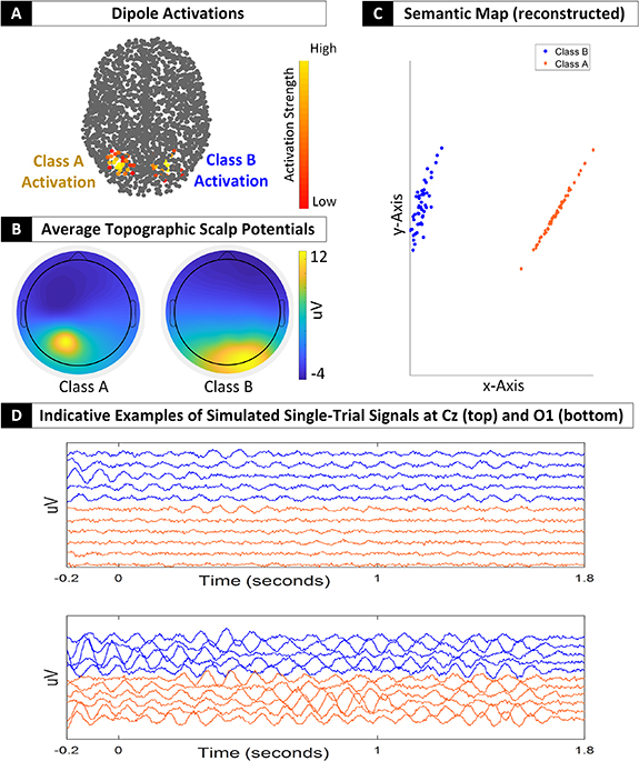
Figure 4. (A) Dipole activations for the two classes of simulated single-trial signals. In the first class an activation pattern appeared on the left occipital dipoles whereas in the second on the right. Color coding (from red to yellow) indicates the strength of the activation pattern. Dipoles colored in gray correspond to pink noise. (B) Topographic scalp potentials for the two classes. They were obtained by calculating the leading eigenvector for the average covariance matrix of each class. (C) 2D semantic geodesic map of the Single-trial covariance patterns. Blue and orange color indicate coavariance matrices of class A and B respectively. (D) Indicative examples of the simulated signals at two sensors (Cz and O1). Blue and orange color indicate single-trial signals of Class A and B respectively.
Download figure:
Standard image High-resolution image4.2. SPD matrix quantization
To demonstrate the new possibilities opened by the reconstruction of covariance matrices under a common eigenspace, we apply the method presented on section 2.3.1. Using the Riemannian k-means method over a set of spatial covariance matrices, we initially uncover a codebook. Since we aim to employ this method in order to perform connectivity-based microstate analysis, for each single-trial a series of covariance patterns is calculated. Then, each of these patterns is assigned to its closest prototype (which is part of the codebook) and in this way the single-trial covariation dynamics are represented by means of a symbolic timeseries.
In order to examine the efficiency of this application, we exploit the recordings of dataset A. Our aim here, is to demonstrate that the concept of SPD matrix quantization is capable to uncover the differences between the passive and the attentive conditions. The time-varying covariance patterns were calculated with a step size equal to 0.1 s and 1 s long window size. Then, the Riemannian k-means algorithm [29] was employed in order to uncover the four (as decided in preliminary analysis) protypical matrices that formed the codebook. Figure 5 depicts the symbolic times-series for the passive and attentive conditions that belong to the same, indicative, subject. Moreover, we present the aggregated distribution of the symbolic-timeseries over the codebook. As it can be seen, the prototypes #1 and #4 are capable of discriminating the attentive and passive single trials. To quantify the aforementioned, we were able to achieve an average classification accuracy of 93% and 94% when the wall appeared on the right and left side respectively. The reported accuracy values are based on a ten-fold cross validation scheme, using linear support vector machines (SVMs), in a subject-specific manner. Although similar classification results were achieved when the original covariance matrices were employed (inferior by 1%, but without a statistically significant difference), it should be noted that the classification time of a reconstructed covariance matrix requires approximately 95% less time compared to an original one.

Figure 5. In the top panel, we present the symbolic timeseries for single-subject trials belonging to dataset A. Each color represents a different prototype. In the bottom panel, the distribution of each condition over the four prototypes is illustrated.
Download figure:
Standard image High-resolution imageTo further demonstrate this approach we generated 100 artificial signals, 3 s long each, according to the model described in section 3.3. All dipole signals were generating pink noise, apart from one that was generating nonstationary alpha-band activity. Half of the simulated trials were characterized by their alpha-band energy which was modulated by a sigmoid function (i.e. increasing energy) whereas the other half had their alpha-band modulated by an inverse sigmoid function (i.e. decreasing energy in alpha band over time). Again, the time-varying covariance matrices were calculated with a step size equal to 0.1 s and 1 s long window size. The key concept here is to illustrate that SPD matrix quantization on the time-varying reconstructed matrices is capable to detect such subtle, time-varying, changes. Figure 6 depicts the colorcoded symbolic times-series for the two aforementioned conditions alongside with their corresponding distributions over the codebook. As expected, the distribution diagrams do not exhibit any significant separability for the two conditions, since, the two conditions differ in the order of appearance of the prototypes. However, the presented quantization, illustrated in the form of color coded time series, follows the trend of the source signals (i.e. energy modulated by a sigmoid function). This serves as a clear evidence that the introduced reconstruction process does not tamper the underlying, simple yet subtle, physiological processes.

Figure 6. On the top side of the figure we present the symbolic time series for the simulated EEG data. Each color represents a different prototype. On the bottom the distribution of each condition over the four prototypes is illustrated.
Download figure:
Standard image High-resolution image4.3. Coding over SPD atoms
In this section we demonstrate the employment of coding over SPD atoms on Dataset A. Our effort is mostly dedicated to demonstrating how the reconstruction of covariance under a common eigenspace paves the way for efficient and easily conceivable neuroscientific explorations that lie on the principles of Riemannian geometry. The key concept here is to approximate each covariance matrix as a supersposition of covariance atoms. Hence, each covariance matrix can be now represented solely by its membership (i.e. the non-negative weights) to the covariance atoms. Therefore, the number of atoms characterizes the dimension of the new, weight space. Although the process of uncovering suitable atoms is very important for neuroscientific explorations, in the presented case the atoms are uncovered by exploiting the Riemannian k-means algorithm.
Figure 7 depicts the 2D semantic geodesic map of the approximated covariance matrices alongside with the 2D semantic map of the weight space under the Euclidean distance. As it can be seen, the 2D semantic geodesic map of the approximated covariance matrices is a highly distorted version of the reconstructed one. This is due to the fact that only two covariance atoms were used for the approximation. However, the approximated covariance matrices exhibit clearer separability characteristics than the reconstructed ones. Moreover, the inspection of the weight space allows us to infer that trials belonging to the passive condition, mostly located close to the y-axis, are clearly characterized by their membership to the second atom. On the other hand, attentive trials cover a more wide spectrum of membership over both of the atoms. We should note, that in both conditions there are several trials (those abiding on the axies) that can be characterized solely by their membership to one of the uncovered atoms. Despite that such interpretations are bound to the method that was employed to uncover the atoms, they clearly demonstrate the implications of this approach on neuroscientific explorations. In practical terms, using linear SVMs on the weight space which is Euclidean and under a ten-fold cross validation scheme, we achieved an average classification accuracy (over the six subjects) of 97% and 96% when the chessboard appeared on the right and left side respectively. These results are on par with state-of-the-art methodologies [34].

Figure 7. 2D semantic geodesic map of the approximated covariance matrices on the left and right respectively. On the right, the semantic map of the weight space is depicted under the Euclidean distance. Since only two atoms were employed in this indicative example, the weight space illustration depicts the obtained approximation weights unaltered. Blue dots correspond to the attentive condition whereas orange to the passive condition of a randomly selected participant.
Download figure:
Standard image High-resolution image
5. Discussion
In this work we presented a methodology that allows the reconstruction of spatial covariance matrices under the assumption of a common eigenspace. The vast majority of our effort is dedicated to showing that the introduced reconstruction process does not tamper the structure of the original covariance manifold. Given its validity, our research aims to bridge the gap between Riemannian geometry and neuroscience. Indeed, Riemannian geometry has been proved to be an invaluable asset in EEG signal analysis (e.g. [46]), however it requires rigorous mathematical procedures that may hinder its wider adoption. Moreover, this problem becomes more acute given that classical pattern recognition and machine learning schemes cannot be readily employed in Riemannian schemes.
In many cases, EEG decoding algorithms are agnostic with respect to the physiological processes that accompany the brain signals (e.g. their origin or the information they may carry) [47, 48]. Here, we aim to offer a valuable insight on the connection of the neural mechanisms that underpin the EEG signals in the context of Riemannian geometry. Although AJD has been previously exploited in this context (particularly for BSS [49, 50]), the pervasive and elusive EEG variability among different individuals have remained, among others, insufficiently explored. Towards this end, we established, that under the assumption of common mixing matrix, one of the most typical transfer learning approaches has a strong neurological basis, that of normalizing the energy of the source signals. Ultimately we believe that our work may further foster neuroscientifically-aware brain decoding algorithms.
In the presented work we show that when the AIRM is employed to deal with spatial covariance matrices, one may reconstruct (exploiting the concept of AJD) these matrices under a common eigenspace and equivalently work with the corresponding eigenvalues. Such a reconstruction offers the advantage of vectorization, where the spatial covariance matrices can be completely characterized by their diagonalized form and consequently be treated as vectors. However, in order to maintain the original structure of the matrices a reformulation of the AIRM and its induced geodesic distance should be employed for vectors, as described in section 2.1.
In addition to the simplifications that the presented methodology brings, it also comes with a second advantage; that of computational efficiency. As a matter of fact inner products and distance calculations under the AIRM have a computational complexity of  . However, working with the equivalent diagonalized forms the corresponding computational complexity reduces to
  . This is a large improvement, especially when dealing with dense EEG recordings or incorporating Riemannian geometry schemes in real-time applications. However, the reduction in computational complexity (e.g. in terms of time cost) can be observed only during the testing phase or when complicated manipulations are required (e.g. in Riemannian geometry-based microstate analysis) subsequent to the diagonalization process. In cases where the classification task is applied only on a few samples (compared to the training set), the reduced testing time cannot compensate for the increased cost induced by AJD. Hence, it becomes obvious that AJD, which is a computationally demanding operation, may cancel out any computational gain achieved by the proposed reconstruction process. A straightforward solution to this shortcoming, concerns the calculation of the common eigenspace only on a small sample of data. This will allow the proposed approach to generalize, at the cost of a less accurate mixing matrix estimation, effectively for the entire dataset. Moreover, the AJD concept can be incorporated as a calibration procedure, since it has to be performed only once, leading to computationally efficient online applications.
The introduced methodology is based on physiologically plausible assumptions that underpin the EEG recordings. Our major assumption concerns the existence of a constant mixing matrix. Despite that this idea is supported by a wide variety of literature, we experimentally show that a 'physiologically ideal' unmixing matrix indeed exists within each recording session. Since the scalp position is stable with respect to the electrodes, it is sound to assume that there should exist a matrix which can approximately and jointly diagonalize the independent physiological sources for all the trials within each session.
One important aspect that has not been discussed particularly in the manuscript concerns the dimensionality of the mixing matrix and its mathematical connections with the employed Riemannian geometry schemes. In a strict mathematical sense, the AIRM-induced geodesic distance is invariant to congruence when the matrix is full-rank. Therefore, equivalence between the sensor space and the source space can be achieved when the number of sources and the number of electrodes are equal (i.e. the mixing matrix is a non-singular square matrix). In practice however, Riemannian geometry has offered significant achievements in EEG signal processing and is still an evolving research field. As discussed in [6], Riemannian geometry in the EEG field is more robust when the number of available sensors is sufficiently enough. This, still unexplored, aspect may limit the implications of both Riemannian geometry generally and the introduced methodology particularly.
As mentioned earlier, bridging the gap between rigorous mathematical procedures and computational neuroscience is among the most profound contributions of this work. Hence, it was within our scope to show the implications of the introduced methodology. To this end, we reformulated and re-introduced two approaches, namely SPD matrix quantization and coding over SPD atoms, in order to showcase the benefits that the reconstruction of spatial covariance matrices under a common eigenspace brings. One important aspect in these two approaches concerns the codebook and atom learning respectively. In both cases we employed a naive algorithm, the Riemannian k-means. This of course may confine the reported results but it was beyond the scope of our work to propose new algorithms for unsupervised learning. Our objective here was to demonstrate the capabilities that open via the introduced reconstruction procedure. We believe, that the presented work may pave the way for robust and efficient neuroscientific explorations that abide to Riemannian geometry.
Acknowledgment
This work was supported by the NeuroMkt project, co-financed by the European Regional Development Fund of the EU and Greek National Funds through the Operational Program 'Competitiveness, Entrepreneurship and Innovation', under RESEARCH CREATE INNOVATE (T2EDK-03661).
Data availability statement
The data that support the findings of this study are openly available at the following URL/DOI: https://github.com/fkalaganis/Riemannian_AJD.
Footnotes
- 3
In rigorous terms, covariance matrices are positive semi-definite whereas strictly positive definite if and only if they are full rank.
- 4
Supplementary data (0.1 MB PDF)