
Abstract
Objective. Technical advances in deep brain stimulation (DBS) are crucial to improve therapeutic efficacy and battery life. We report the potentialities and pitfalls of one of the first commercially available devices capable of recording brain local field potentials (LFPs) from the implanted DBS leads, chronically and during stimulation. The aim was to provide clinicians with well-grounded tips on how to maximize the capabilities of this novel device, both in everyday practice and for research purposes. Approach. We collected clinical and neurophysiological data of the first 20 patients (14 with Parkinson's disease (PD), five with dystonia, one with chronic pain) that received the Percept™ PC in our centres. We also performed tests in a saline bath to validate the recordings quality. Main results. The Percept PC reliably recorded the LFP of the implanted site, wirelessly and in real time. We recorded the most promising clinically useful biomarkers for PD and dystonia (beta and theta oscillations) with and without stimulation. Furthermore, we provide an open-source code to facilitate export and analysis of data. Critical aspects of the system are presently related to contact selection, artefact detection, data loss, and synchronization with other devices. Significance. New technologies will soon allow closed-loop neuromodulation therapies, capable of adapting stimulation based on real-time symptom-specific and task-dependent input signals. However, technical aspects need to be considered to ensure reliable recordings. The critical use by a growing number of DBS experts will alert new users about the currently observed shortcomings and inform on how to overcome them.
Export citation and abstract BibTeX RIS

Original content from this work may be used under the terms of the Creative Commons Attribution 4.0 license. Any further distribution of this work must maintain attribution to the author(s) and the title of the work, journal citation and DOI.
1. Introduction
Deep brain stimulation (DBS) is a common practice for the treatment of many neurological conditions (e.g. Parkinson's disease (PD), dystonia, essential tremor) [1, 2]. Despite impressive technological advances over the past 30 years, stimulation therapies are still restricted to continuous stimulation protocols that are tuned manually during in-clinic visits. This lack of adaptability fails to address essential disease-, medication-, and activity-related fluctuations of the clinical condition. To address these limitations, next-generation neurotechnologies are being developed to operate in closed-loop [3–5]. These devices offer the possibility of automatically adapting stimulation parameters in response to feedback signals, chronically and in real time. Emerging evidence suggests that adaptive stimulation approaches may exhibit greater efficacy with fewer adverse effects [6–8]. However, translation of such strategies into everyday life is yet to be achieved [9], and strongly relies on the user-friendliness, quality, and robustness of the sensing capabilities endowed in chronic devices.
Recently, new implantable devices capable of chronically recording local field potentials (LFPs) during stimulation became available [10, 11]. Their sensing capabilities should enable better understanding of disease-related brain activity patterns, their evolution over time, and their modulation in response to therapies, bringing the implementation of adaptive stimulation therapies closer to clinical practice.
Here, we report the potential applications and pitfalls that emerged when using Percept™ PC (Medtronic PLC, USA) in the first 20 patients implanted at our centres. We provide relevant surgical, technical, and operational aspects to be considered to maximize its performance and signal quality in the clinical practice and in clinical research contexts. The aim of this report is to share insightful views coming from our early experience, in order to provide clinicians who plan to use this novel device with practical tips to optimize and facilitate its use.
2. Methods
2.1. Patients
We collected clinical and neurophysiological data for the first 20 patients (14 PD, five dystonia, one chronic pain; 12 males) that received the Percept PC at our three centres. Patients were not selected based on specific characteristics and the implant was performed in the context of clinical practice.
The severity of PD and dystonia symptoms was assessed using clinical rating scales by an experienced movement disorders clinician, as part of the clinical routine (supplementary table 1 available online at stacks.iop.org/JNE/18/042002/mmedia).
2.2. Surgical procedure
Four patients received the Percept PC during replacement of their implantable pulse generator (IPG). All others received it simultaneously to lead implantation or 5 days afterwards (two patients) (supplementary table 1). In one patient (PW4), the IPG was implanted in the right abdominal region; in all others it was implanted in the chest (left: NL1, NL2, PW2–3; right: CH1–10, PW1, 5–8, PW1A).
All patients but CH10 received bilateral leads (3389, Medtronic, PLC, USA) with four cylindrical contacts. By convention, and in order to reflect the extraction files structure of the Percept PC, the lowermost contacts of each lead are labelled 0, and uppermost contacts are labelled 3 for either side. For example, 0–2 L designates the contact pair 0 and 2 of the left side, 0–2 R designates the contact pair 0 and 2 of the right side, etc. Patient CH10 (with refractory chronic pain in the left hand) received two quadripolar electrocorticography (ECoG) strips (Resume II, four contacts per lead) for epidural right motor cortex stimulation.
The surgical procedure of each centre has been previously reported [12–15]. No specific procedures were followed for Percept PC implantation. The proper lead placement in the subthalamic nucleus (STN) for PD patients and within the Globus pallidus internus (GPi) region for dystonic patients was checked by means of intraoperative microelectrode recordings and test stimulation, and by image fusion of pre- and postoperative scans. A standard silicon sleeve (Medtronic PLC, USA) was used to cover the connection between the lead and extension cables, and fixed it with one stich on the distal end (Haga/LUMC) or two stitches at the proximal and distal end (CHUV, UKW). The lead was fixed to the skull with a silicon cap (StimLoc, Medtronic, PLC) (UKW, LUMC) or with cement (Palacos R+G, Heraeus Medical, Germany) (CHUV).
2.3. Patient recordings
The Percept PC can continuously record LFP in real time, also during active stimulation, and transmit them wirelessly to a storage device (a tablet—user interface). Bipolar recordings can be performed in several modes (BrainSense™, table 1). Data can be partially visualized online (figure 1) and saved.

Figure 1. Online evaluations using BrainSense™. (A) Screenshot of the Percept™ PC user interface (tablet) displaying the PSD generated in the BrainSense survey modality (patient NL1, left lead, meds-off condition). The highest beta power could be identified between contacts 1 and 3. Monopolar stimulation from contact point 2 had the best effect but induced dyskinesia, thus contact 1 was chosen for chronic stimulation. (B) Online visualization of LFP power sensing for a pre-selected frequency band in the BrainSense streaming mode (one new datapoint visualized every 500 ms), while manually increasing stimulation amplitude (patient CH5, right STN). Increase in stimulation amplitude induced a decrease in beta-band power after reaching 2 mA. Concurrent clinical motor evaluations confirmed improvements in rigidity associated with LFP beta power modulations.
Download figure:
Standard image High-resolution imageTable 1. Main functions and features of the available recording modes with the Percept™ PC device.
| Recording modes | Stimulation | Use | Contact pairs | Main functions and features | |
|---|---|---|---|---|---|
| BrainSenseTM survey | Survey | Off | In clinic | All possible contact pairs (figure 1(A)). |
|
| Survey indefinite streaming | Off | In clinic | All stimulation-compatible contact pairs (e.g. 0–3, 1–3, 0–2) |
| |
| BrainSenseTM streaming | Setup | Off or on | In clinic | All possible contact pairs |
|
| Streaming | Off or on | In clinic | A single pre-defined contact pair for each hemisphere (if both have a complete Setup) |
| |
| Timeline | Off or on | At home | Preselected contact pairs (dependent on active stimulation contact) |
| |
| |||||
| Events | Off or on | At home | Preselected contact pairs (dependent on active stimulation contact) |
| |
The timing of recordings with respect to implant, medication and stimulation state, and recording modality used are reported in supplementary table 1 for all patients.
In three patients (NL1, NL2, and CH6) at-home chronic recordings were performed with Timeline modality during several days. For purpose of demonstration, one patient (CH6) was asked to mark events of freezing of gait. In addition, in-office recordings were performed.
For Haga/LUMC subjects, recordings were obtained in the context of routine monopolar contact review, and subsequent outpatient evaluations.
For all UKW subjects but one (PW4), we collected LFP during the eyes-open resting state. LFP of patient PW4 were acquired during unperturbed walking with Streaming mode in a gait laboratory environment [14, 16, 17]. This patient was asked to stand quietly and to start walking over an 8 m long walkway after a verbal cue. The task was repeated four times. Body kinematics was measured with a full-body marker set and a motion capture system (SMART-DX, BTS, Italy). [18–20] Recordings in PD patients were performed after overnight suspension (>12 h) of all dopaminergic drugs and after pausing the stimulation for 30–60 min. The duration of each recording session was 90–120 min. In one case (PW1, figure 2(B)), we also performed the recordings in meds 'on' and 30 min after switching the stimulation on at the clinically effective parameters. In patients with dystonia, we aimed for a longer pause of DBS (72 h for PW4, 5, 1 A, 8 and 12 h for PW6). Dystonic patients were not taking medication during the recordings.
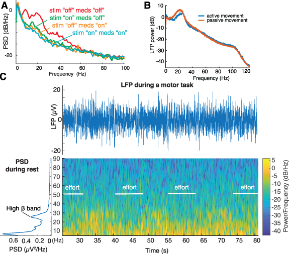
Figure 2. Offline evaluations of high-resolution LFP recordings modulated by medication, stimulation, and movement. (A) PSD estimates of resting state recordings (patient PW3, sitting with eyes open) in four different conditions: meds 'off' (overnight suspension of all dopaminergic drugs), meds 'on' only (1 h after intake of a standard levodopa dose), stim 'on' only (stimulation with optimal amplitude, 180 Hz), and combined stim 'on' and meds 'on'. Suppression in beta power is captured both in the stimulation-only and medication-only conditions, and with the cumulative effect of both medication and stimulation. (B) Average LFP power estimate recorded from cortical strips placed over the motor cortex during a passive or an active movement of the contralateral arm (CH10). We observed a suppression of beta power during active movement compared to passive movement. (C) Raw LFP signal and Welch's PSD estimates of BrainSense survey indefinite streaming recordings at rest and spectral changes over time during iterative movements (knee extension movements while sitting, patient CH6, right STN, contacts 0–2, meds 'off' and stim 'off'). Unprocessed LFP and spectrogram accurately captured expected movement-related changes in beta power.
Download figure:
Standard image High-resolution imageFor all CHUV subjects, we collected LFP for at least 1 min in the eyes-open resting state, using the Survey indefinite streaming mode (CH1–4, 6–9) or the Streaming mode (CH5). Additionally, we recorded modulations during a motor task (i.e. knee extension movements while sitting) in the Survey indefinite streaming mode (CH1–4) or the Streaming mode (CH5–9—figure 2(C)).
To synchronize Percept PC recordings with other devices for monitoring electrophysiological signals (i.e. muscular electromyography (EMG) and cortical electroencephalogram (EEG) data, we explored two methods:
- (a)In two patients, we induced DBS artefacts in Streaming mode. Specifically, we turned the stimulation briefly 'on' and 'off' at the beginning of the recording to produce an artefact simultaneously visible in the LFP and other data streams. This artefact was then used as a reference point to align the signals. In patient CH5, the stimulation artefact was captured by an EMG probe (DTS EMG, Noraxon) with one electrode (ECG electrode, H124SG, Kendall) placed on the clavicle, the other placed over the IPG. In patients PW6, we captured the DBS artefact (2.0 mA, 110 Hz, 90 µs) simultaneously with a wireless EMG probe (FREEMG, BTS, Italy) placed on the neck in correspondence of the extension cable connecting the IPG and the leads, and with a 64 channel wireless device for EEG recordings (Sessantaquattro, OT Bioelettronica, Italy). To optimize the detection of the synchronization artefact in the EEG data stream, we selected across the 64 channels the one with the highest variance. Synchronization across all signals (i.e. LFP, EMG, EEG) could then be achieved offline by aligning the data to the sharp drop of the stimulation artefact.
- (b)Following our past experience with the Activa PC+S device (Medtronic PLC, USA) [14, 16, 17, 21], we explored the possibility of recording electrical artefacts produced by a transcutaneous electrical nerve stimulator (TENS) for synchronization purposes in research applications. The company recommends not to place TENS electrodes so that current might spread over any part of the neurostimulation device, as TENS currents are considered potential sources of electromagnetic interference with the implanted stimulator. However, no issues or adverse effects in this regard have been reported so far. In two patients, we induced a TENS artefact while recording in Indefinite streaming mode. Two surface electrodes (Neuroline 715, Ambu, Ballerup) were placed on the neck of two patients (CH5 and CH10) over the lead extension and on the contralateral mastoid for the delivery of the TENS. An EMG probe (Trigno Avanti Sensor, Delsys) was placed on the neck. Multiple 1 s TENS bursts (1 ms pulse width, 1.5 mA, charge-balanced square pulse, 80 Hz, interleaved with 1 s pause) were sent with an external stimulator (NIM-Eclipse™ E4, Medtronic PLC). Synchronization across data was achieved by aligning the onset of an LFP artefact to the onset of the corresponding EMG burst. No stimulation burst appeared on the raw LFP signal (figure 12(B)). Yet, the burst could be identified by computing the power of the 80 Hz band (Butterworth band pass filter, order 2, 78–82 Hz) (figure 12(D)). However, the onset of the burst cannot be precisely identified as the filter introduces a temporal smoothing. To find the actual onset time of the LFP artefact, we identified the LFP contact pair displaying the highest power on the 80 Hz band, and set an arbitrary power threshold on the band. Then we identified the middle of the burst as the point halfway between the initial and last threshold crossing. As each TENS burst was sent with a defined duration of 1 s, we could infer the actual start of the LFP burst as being 0.5 s before the middle of the burst. In the EMG recordings, we manually labelled the start of the bursts as the onset of the stimulation artefacts. Of note, pre-defining the burst duration is not necessary (e.g. if the TENS is not able to send a burst of a controlled duration), as it could be inferred by measuring the burst duration in the EMG recordings.
2.4. Data analysis
For analysis, data were exported in a JavaScript Object Notation (JSON)-format file (figure 2). Since the software to read and analyse the JSON files is not provided, we imported the data into MATLAB (Mathworks, Natick, MA) with a custom-built toolbox, and analysed it using custom-built code (available at https://github.com/YohannThenaisie/PerceptToolbox.git).
All raw LFP recordings were visually inspected for cardiac-related artefacts. To remove the cardiac artefact, we computed the singular value decomposition of LFP data epoched around the QRS peaks. The component resembling the QRS complex was visually identified (namely the ones explaining more than 97.5% of the variance) and subtracted from the raw data [17].
In PD patients, beta-band analysis was performed on Survey indefinite streaming or Survey data (supplementary table 2, figure 3). For each Survey indefinite streaming, we reconstructed bipolar LFP signals from adjacent contacts by subtracting the signals of recorded channels as extracted from the JSON file as: LFP0–1 = LFP0–3 − LFP1–3, LFP1–2 = LFP1–3 + LFP0–2 − LFP0–3, LFP2–3 = LFP0–3 − LFP0–2, similarly to standard EEG montages. Power spectrum density (PSD) estimates were computed via Welch's method (pwelch function). We defined the frequency of the beta peak fPeak as the frequency with the local maxima power in the 13–35 Hz range. We visually verified each PSD for the presence of beta (13–35 Hz) and gamma (60–90 Hz) bands. For each STN, we reported the contact pair with the highest fPeak power in the beta band. Short-time Fourier transform was applied on raw LFP from all Streaming recordings (supplementary table 1).

Figure 3. Beta peak frequency and power in all contact pairs of 22 STNs recorded with Survey and Survey indefinite streaming modalities during resting. (A) Power of the beta peak in all contact pairs of 22 STN, normalized by STN. A contact pair is displayed as black when no peak could be identified in the beta range (13–35 Hz). For each STN, the contact pair with the maximum beta peak power is labelled with a star. (B) Peak frequency of the contact pair with the highest beta power for the 19 STN in which the beta peak was identified in at least one contact pair. The horizontal dashed line indicates the average beta frequency of all STN. (C) Number of times each of the contact pairs was identified as the one with maximum beta power across the 19 STN in which a beta peak was present.
Download figure:
Standard image High-resolution imageIn dystonic patients, theta–alpha band analysis was performed on Survey data. We reconstructed bipolar LFP signals from adjacent contacts as described above. PSD was computed using Welch's method and 1/f component removal [21]. For each contact pair, PSD was normalized for the standard deviation computed between 6 and 96 Hz to minimize spectral contamination due to movement artefacts (e.g. phasic dystonic movements and myoclonic jerks) [22]. Artefact-free recordings as identified by the Percept PC were visually inspected for peaks in the theta–alpha band (4–12 Hz) (figure 4). In patient PW5 we performed three consecutive Survey recordings and evaluated and compare the movement artefacts (supplementary figure 1). LFP data were synchronized with kinematic tracks and epoched in 800 ms windows centred at the heel contacts (HCs), detected as the local minima of the markers tracks placed on the heels (figure 10).
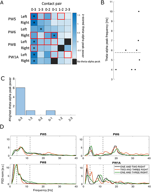
Figure 4. Theta–alpha peak frequency and power in all contact pairs of eight globus pallidus internus (GPi) recorded using the Survey mode during resting. (A) Power of the theta–alpha peak in all contact pairs of eight GPi nuclei, normalized by GPi. A contact pair is displayed as black when no peak could be identified in the theta–alpha range (4–12 Hz). For each GPi, the contact pair with the maximum theta–alpha peak power is labelled with a star. Red boxes indicate contact pairs labelled as artefactual by the device. (B) Peak frequency of the contact pair with the highest theta–alpha power for all GPi. The horizontal dashed line indicates the average theta–alpha peak frequency of all GPi. (C) Number of times each of the contact pairs was identified as the one with maximum theta–alpha power across the eight GPi. (D) PSD of local field recordings (LFP) recorded by contact pairs labelled as non-artefactual in all patients. Vertical dashed lines indicate the theta–alpha band. A peak in the theta–alpha band was evident in patients PW5, PW6, and PW1A from all recording pairs, and present also in recordings of PW8 even if less prominently. Patient PW6 also showed a prominent peak in the beta band.
Download figure:
Standard image High-resolution image2.5. In vitro recordings
For in vitro tests, a DBS lead (3389) was inserted in a paper towel soaked in a saline solution (Phosphate-buffered saline pH 7.4 1×, 10 010, Gibco) and connected to the Percept PC.
The Percept PC recording device uses a nominal sampling frequency of 250 Hz, and contains two low-pass filters at 100 Hz and two high-pass filters at 1 Hz, and 1 or 10 Hz (user-defined) [23]. Because the previous prototypal device Activa PC+S (Medtronic PLC, USA) showed variable sampling frequency, we preliminarily tested the sampling frequency Fs of Percept PC in vitro. To do so, we generated a sinusoid signal (10 Hz, 500 mV) with a function generator (Agilent 33210A LXI) and recorded in Indefinite streaming mode for ∼74.5 s in the saline bath. Offline, we counted the number of oscillations and samples, and computed Fs = (number of samples)/(number of oscillations) × (frequency of oscillations).
Other tests were aimed at evaluating stimulation artefacts and compare them with those observed in patients and validating the synchronization methods.
For these purposes we stimulated with different stimulation amplitudes while recording simultaneously in Streaming mode with Percept PC and with an external amplifier at 24 414.06 Hz (RZ5D BioAmp Processor, Tucker Davis Technologies, USA). Signals from both systems were synchronized by sending an external 10 Hz sinusoidal signal generated with Agilent 33210A LXI at 100 mA for a few seconds.
2.6. Ethics
The Medical ethical committee Leiden Den Haag Delft, the Ethik-Kommission of the University Hospital Würzburg and the Ethical Committee of the Canton of Vaud approved the respective studies and/or waived review for the data collection of the respective centre.
All patients gave written informed consent according to the Declaration of Helsinki.
3. Results
We report here our considerations concerning the recording of biomarkers of potential clinical relevance and some advices and recommendations for successfully recording LFP signals with the Percept PC device (summarized in table 2).
Table 2. General considerations to improve LFP recordings with the Percept™ PC device.
| Tips and tricks | |
|---|---|
| Recording procedure and data export: How to avoid data loss |
|
| Synchronization with other devices Possible methods |
|
| Artefacts management |
|
3.1. In-clinic recordings
3.1.1. Recordings of STN beta oscillations in PD
A beta peak was identified in 19/22 STN for which the Survey or Survey indefinite streaming mode was available, at an average frequency of 22.6 Hz (SD ± 4.9 Hz) (figures 3(A) and (B)). In three STN, no contact pair displayed a beta band. In 13/19 STN, the maximum beta peak was found in contact pair 1–3 or 0–3 (figure 3). In all but three STN (of three different patients), the clinically chosen contact for chronic stimulation was either in between or one of the contact pairs displaying the maximum beta peak (supplementary table 2). In some patients, we could also identify a stimulation amplitude-dependent modulation of the beta power (figure 1(B), supplementary figure 2), concomitant with clinical improvement of rigidity. We could also confirm that the Percept PC captures modulations in beta power induced at rest by STN-DBS and levodopa alone or in combination (figure 2(A)). Finally, we could record the expected changes in beta power induced by movements during a motor task off medication and off stimulation (figure 2(C)).
3.1.2. Recordings of GPi theta–alpha oscillations in dystonic patients
A theta–alpha peak was identified in all the eight GPi nuclei analysed (94% of all the available contact pairs, 91% of the non-artefactual contact pairs). For each patient and hemisphere, we considered the contact pairs with maximum theta–alpha peak and computed an average frequency of 5.7 Hz (SD ± 2.1 Hz) (figure 4). In 6 out of 8 GPi, the maximum theta–alpha peak was found in contact pair 0–3. In these recordings, 27% of the contact pairs were labelled as artefactual by the Percept PC (see below). Consecutive Survey recordings showed high variability of LFP measurements. The signal recorded in the same patient (PW5) by the same contacts during consecutive sessions was differently identified as artefactual or non-artefactual (supplementary figure 1), possibly due to episodic movement artefacts.
3.1.3. Recordings of motor cortex LFPs with ECoG strips in one patient with chronic pain
The left arm of one subject (CH10) was actively or passively moved while we recorded LFP from the ECoG strips implanted on the contralateral motor cortex. The Percept PC system successfully captured lower beta band power during active movements compared to during passive movements (figure 2(B)).
3.2. At-home recordings
In all three PD patients with Timeline chronic recordings, we observed circadian and daily power fluctuations of the preselected beta band during the whole recording duration (up to 49 d) (figure 5). Beta power was suppressed overnight, which we assume corresponds to sleep time. Some fluctuations were present during the day. One patient was asked to mark Events during freezing of gait episodes. The Percept PC successfully computed bilateral PSD estimates over a ∼30 s window following each marked Event (figure 6(C)). There was no consistent Event-related modulation of the recorded PSD, suggesting multiple possibilities: (a) (most likely) the Event was not actually marked during a freezing episode (e.g. due to the short duration of the freezing episode and the time needed to reach for the programming device/smartphone and mark the event), (b) there were no freezing-related PSD modulations, or (c) the Percept PC was not capable to capture these modulations.

Figure 5. At-home recordings and marked events Recordings performed with the Timeline modality in patient CH6. A frequency band in the beta range (23.39 Hz) was selected by the clinician to be chronically monitored in 'passive mode' by contact pair 1–3 L. Stimulation was 'on' on contact 2 L at the optimal therapeutic value (2.9–3.2 mA). (A) LFP band power between 48 d (D + 48) and 97 d (D + 97) after surgery. (B) Three-day close-up view of the recording in (A). Circadian and daily fluctuations in power are evident, including power depressions at night. In addition, the patient manually reported freezing of gait events (purple lines) on their patient controller. (C) Example PSD of an event reported by the patient (left STN displayed only). This data is only proposed as a representation of this function (see text).
Download figure:
Standard image High-resolution image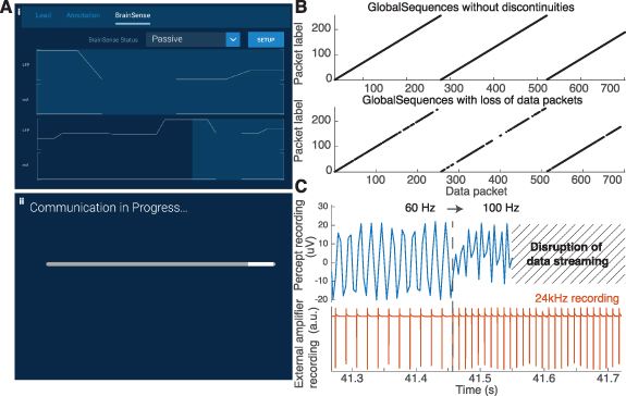
Figure 6. Data-packet loss due to transmission failures, and data re-alignment. (A) We encountered two main data transmission problems, which would display either (i) a discontinuity in the data trace display, and resulted in a loss of packets, or (ii) a loading bar indicating communication difficulties, which resulted in the data recording being cut in two matrices. (B) The presence and location of missing data packets could be inferred (and corrected) from the exported JSON file. The fields 'GlobalSequences', 'TicksInMses', and 'GlobalPacketSizes' provided the necessary information to ensure a proper alignment in time, even in presence of missing data. (C) Changes in the frequency of stimulation temporarily terminated the data transmission, and automatically started a new recording after 5 s, resulting in data loss. Tests in saline water confirmed that changes from 60 to 100 Hz during a recording (1.0 mA, 60 μs) resulted in such disruption in the recording.
Download figure:
Standard image High-resolution imageFor each marked event, the Percept PC successfully computed bilateral PSD estimates over a ∼30 s window following each marker.
3.3. Sampling frequency (in vitro)
Base on the in vitro experiments, we computed the sampling frequency to be 249.7 Hz (over 745 oscillations). This confirms the manufacturer's nominal value (Fs = 250 Hz).
3.4. Size and structure of exported files
Each session may be exported as one JSON file for offline analysis. Importantly, multiple consecutive recordings within the same session are appended and saved in a unique JSON file during export, which may make it difficult to later identify the single recordings.
We observed that recordings longer than 10 min (exported before December 2020) resulted in export failures and data loss, possibly due to excessively large files. Furthermore, there was no correspondence between the user interface (tablet) recording names and times and the names attributed to the JSON files, which were identified by a timestamp with the date and time of the export from the tablet (and not of the recording). The time of start and end of the recording is saved within the JSON file.
3.5. Data loss during online streaming
We encountered two situations of temporary loss of data streaming
- (a)The data stream lost a few data packets, but the recording was not interrupted. Such events can be observed as an interruption of the continuous LFP line displayed on the tablet (figure 6(A)(i)). We experienced data-streaming loss when the Communicator (positioned onto the IPG) and the Tablet were >3–5 m apart, or when an obstacle (including the patient's body) was in-between. Of note, data appeared as a continuous matrix, without indication of the missing samples in the JSON file.
- (b)The data stream was temporarily interrupted (figure 6(A)(ii)). This can happen when the Communicator and Tablet or IPG are far from each other, or when changing the stimulation frequency or programming group with active Streaming mode (figure 6(C)). In this case, data recorded after the interruption was stored in a new data matrix after the streaming was retrieved. No data packet was lost when changing the stimulation amplitude during active Streaming mode.
In both situations, the missing data could not be retrieved. Moreover, streaming disruptions jeopardized the alignment of the LFP recordings with other devices. Fortunately, the JSON file contained the timestamps of the received data packets (TicksInMses) and the number of samples of each data packet (GlobalPacketSizes) (figure 6(B)). These two metainformation could be used to infer the time and duration of streaming disruptions and restore time synchronization with other devices. We provide a Matlab Toolbox for this purpose (see section 2).
3.6. Artefact detection
3.6.1. Stimulation-related artefacts (in patients and in vitro observations)
For stimulation frequencies below the Nyquist frequency (125 Hz), a stimulation-related peak artefact corrupted the PSD at the corresponding frequency and its ascending harmonics (figure 7). For stimulation frequencies above the Nyquist frequency (i.e. 130 Hz and above), we also measured stimulation artefacts but at lower frequencies (figure 7). This effect is due to aliasing and is characterized by: artefact frequency = sampling frequency – stimulation frequency. These in-patient observations were verified in a saline bath setup, by comparing Percept PC signals with recordings performed using a high-resolution amplifier that is not limited to 125 Hz Nyquist frequency (figure 7(C)). The amplitude of these artefacts decreased as the stimulation frequency increased from 125 Hz upwards. This could be an effect of the 100 Hz low-pass filter.

Figure 7. Stimulation aliasing artefacts. (A) PSD estimate of LFP signals during a rest recording with contact pair 0–2 R with continuous 130 Hz deep brain stimulation (1 R-C+, 1 mA, 60 μs) in Streaming mode (patient CH6). A power peak corrupted the spectrum at 120 Hz (According to the formula artefact frequency = sampling frequency (250 Hz) − stimulation frequency). (B) PSD estimates in saline water during Streaming recordings, for stimulation profiles of four frequencies (60, 100, 130, and 180 Hz). Stimulation under the 125 Hz Nyquist frequency (i.e. 60, 100 Hz) induced power peaks at the stimulation frequency and potential harmonics. Stimulation at 130 Hz induced an artefact at 120 Hz. No artefacts were apparent during 180 Hz stimulation. (C) We stimulated in saline water at various frequencies (1.0 mA, 120–140 Hz, 60 μs) while recording with the Percept PC in Streaming mode and with an amplifier of 25 kHz sampling frequency. Stimulations above 125 Hz induced artefacts at frequencies symmetric to 125 Hz in the Streaming recording only. For example, stimulation at 130 Hz (5 Hz above the Nyquist frequency) induced artefacts at 120 Hz (5 Hz below). (D) In saline water, the power of the artefact peak observed on Streaming recordings decreased as the stimulation frequency increased from 125 Hz upwards (1.0 mA, 125–140 Hz, 60 μs).
Download figure:
Standard image High-resolution imageAt high amplitudes, in two patients (NL1 and CH5), we also recorded stimulation-related subharmonics. In patient NL1, stimulation of contacts 1 L and 2 L induced narrow power peaks in the gamma band at half (i.e. 64.9 Hz), one-quarter (32.5 Hz) and three-quarters (97.4 Hz) of the stimulation frequency in the ipsilateral recording only, starting above 2.5 mA and stopping abruptly when stimulation amplitude is turned to 0 mA, simultaneously with dropping of the 120 Hz artefact. (Figure 8) stimulation of contacts 1 R and 2 R induced a single power peak at half the stimulation frequency above 3 mA and at 2.9 mA, respectively (data not shown). The patient had no dyskinesias during the recordings but developed stimulation-related dyskinesia with chronic stimulation from contact 2 L. At the last follow-up visit, the patient did not show any dyskinesia, but the stimulation-related signals were still present (data not shown).
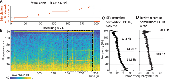
Figure 8. Subharmonic artefacts appearance above a stimulation amplitude threshold. Aligned stimulation amplitude profile (A), LFP spectrogram (B), and PSD estimate (C) (computed between 200 and 290 s) recorded by contact pair 0–2 L during monopolar contact review of contact 1 L at 130 Hz, 60 μs and with a stepwise increment of stimulation amplitude from 0 to 4 mA, off-medication (patient NL1). Stimulation at amplitudes of 2.5 mA and above induced peak power activities at 35.5, 64.9, and 97.4 Hz, which abruptly stopped when stimulation amplitude was lowered to 0 mA. The 125 Hz symmetrical artefact at 120 Hz is also visible and is already present with the stimulator turned on at 0 mA. No dyskinesias were observed during the recording. Similar findings were recorded when stimulating with contacts 2 L, 1 R, and 2 R, and recording from 1–3 L, 0–2 R, and 1–3 R respectively (data not shown). (D) We stimulated saline water at 5 mA, 130 Hz and 60 μs, while recording in Streaming mode. Only 50 Hz (electrical line power) and 120 Hz (stimulation artefact) power bands are visible in this setup.
Download figure:
Standard image High-resolution imageIn patient CH5, in a similar setup, only one subharmonic oscillation peak at half the stimulation frequency was recorded (besides the 120 Hz artefact), starting from 4 mA, and only when stimulating through contact 1 R (sensing pair 0–2 R). The patient did not display dyskinesia during the recordings (supplementary figure 2).
To investigate the nature of these artefacts, we replicated the experiment in a saline setup and recorded no subharmonic oscillations (figure 8). We cannot exclude a biological nature for these stimulation-related signals.
3.6.2. Cardiac-related artefacts
Cardiac artefacts notably affected the power of the beta range [10] and were observed in at least one contact pair in four patients (20%), two of which with the IPG implanted on the right chest (supplementary table 3).
We observed two categories of cardiac artefact
- (a)In three patients (NL1, NL2, and PW1), we observed cardiac artefacts in Streaming or Setup modes when stimulation was on (even at 0 mA) but not when stimulation was off. The artefacts were absent in Survey mode. Monopolar impedances of the artefactual and stimulation contacts were all in acceptable range (between 785 and 1643 Ω) and we did not observe an imbalance of impedance between an artefactual recording contact and its corresponding stimulation contact (difference range 9–495 Ω) (supplementary table 3). The manufacturer suggested that these artefacts may be linked to the involvement of the stimulation contact in the sensing circuitry that might arise from fluid leakage, typically at the leads-extensor connector.The cleaning process effectively removed the QRS peaks from the raw signal, likely preserving the signal neural content (figure 9).
- (b)In one patient (CH6), we observed cardiac-related artefacts with Survey indefinite streaming, Setup and Streaming mode recordings (stimulation 'off' and 'on').
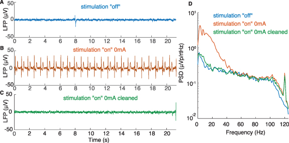
Figure 9. Cardiac artefacts. Illustrative example of LFP signals recorded with Setup in the stimulation 'off' (A) and stimulation 'on' (0 mA) (B) conditions (patient NL1, contact pair 1–3 R) in the early postoperative period. The inclusion of the active contact (monopolar configuration, referenced to the IPG case), even at 0 mA, immediately induced cardiac-related artefacts that corrupted the raw signal and covered most frequencies under 50 Hz in the PSD estimate (D). The cleaning process effectively removed the QRS peaks from the raw signal (C). The resulting PSD shows a decrease in the frequency content between 1 and 40 Hz, the range typically affected by the cardiac artefact (D). The similarity between the PSD in stim 'off' and cleaned 'on' conditions suggests that the neural content of the signal was mainly preserved after processing.
Download figure:
Standard image High-resolution image3.6.3. Movement-related artefacts
There was an evident gait-related movement signal in the right hemisphere recordings of PW4 (IPG in the right abdomen) while recording in Streaming mode 'off' stimulation (figure 10). Its presence in one hemisphere only and the lack of relation with the corresponding stepping leg supports the hypothesis of the artefactual origin of these oscillations, rather than a gait-related neural modulation. No cardiac-related artefact was present in these recordings. Impedances were within the normal range for all contact pairs. This artefact's origin remains unclear; IPG location may play a role, but is probably not the only factor of influence [10]. Of relevance, such an artefact was visible exclusively when recordings were epoched to specific events of the gait cycle, i.e. heel strike. We cannot exclude the presence of artefacts during other motor tasks, and LFP recordings with Percept PC during movement should thus be carefully evaluated.
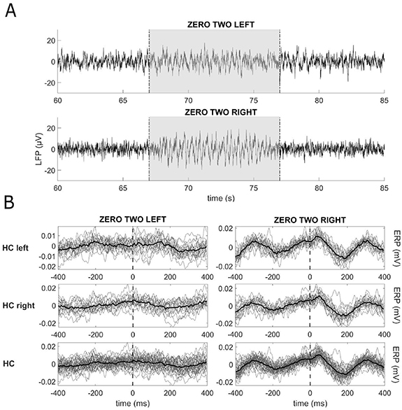
Figure 10. Movement-related artefacts during walking. Recordings from one dystonic patient (PW4) during walking. (A) Raw data of LFP recordings in Streaming mode in stimulation 'off' from contact pairs 0–2 L and 0–2 R. The grey area identifies the walking window (from about 67 to 77 s), preceded and followed by quiet standing. Movement-related artefacts are visible in the raw signal. (B) LFP of 4 walking trials epoched in 800 ms windows centred at the heel contacts (HCs) (vertical dashed lines), as detected by the kinematic assessment. In total, 37 epochs of gait were analysed. The left and right columns show the data of the left and right hemispheres epoched with respect to the left (first line) and right (second line) HCs, and to all the HCs (third line). In each subpanel, the grey lines represent the LFP recorded in each epoch and the thick black line represents the average across all epochs. We found a modulation on the right hemisphere only, not related to the side of the on-going stepping.
Download figure:
Standard image High-resolution imageSpike-like artefacts were also noticed in recordings identified as non-artefactual by the Percept PC (supplementary figure 1(B)). This is possibly related to the transient and episodic nature of dystonic and myoclonic jerks, which might be variably captured by the Percept PC. Longer recordings (with Survey indefinite streaming and Streaming) might be more robust against movement artefacts for PSD computation, especially when estimating theta–alpha activity, and might facilitate proper contact selection for chronic sensing (supplementary figure 3).
3.7. Synchronization of the Percept PC with other devices
Synchronization input/output signals are not presently available within Percept PC. We tested two alternatives for synchronization in the Survey indefinite streaming and in the Streaming mode; alignment may only be performed offline.
3.7.1. Electrical artefact induced by the DBS (in patients and in vitro observations)
A sudden change of the stimulation amplitude of the Percept PC can be picked up by external devices such as an EMG sensor placed over the IPG or an EEG (figures 11(A) and (B)). Unfortunately, the stimulation amplitude data stored by the Percept PC has a low sampling frequency (2 Hz) and is imprecise (figure 11(A)). Therefore, this data should not be relied on for synchronization.

Figure 11. DBS artefacts can be used to synchronize recordings in the Streaming modality with EMG and EEG recordings. (A) A change in DBS amplitude (from 1.3 to 0 mA, 130 Hz, 60 µs—top) induced an artefact recorded by BrainSense™ streaming (middle) in patient CH5. In addition, a bipolar surface EMG captured single-pulse artefacts. Therefore, Streaming and EMG recordings could easily be aligned (vertical dashed line). Note the temporal inaccuracy of the stimulation amplitude stored at 2 Hz (top): the stimulation amplitude stored in Percept PC indicated that stimulation changed 70 to 570 ms before the actual stimulation change. (B) Recordings from the two LFP channels (left and right), one EMG channel, and EEG channel FT10 while bilateral stimulation (2.0 mA, 110 Hz, 90 µs) was turned 'on' and 'off' in BrainSense streaming mode in patient PW6. A ∼0.5 s long transition artefact was evident on the LFP recording when stimulation was turned on and, with opposite polarity, when the stimulation was switched off. Both EMG and EEG clearly show stimulation-related bursts as DBS was turned on. Synchronization could then be achieved offline by aligning the signal to the sharp drop of the stimulation artefact. (C) In saline water, the stimulation amplitude was changed from 0 to 1 mA and from 1 to 0 mA (130 Hz, 60 µs) while simultaneously recording with Streaming and a synchronized high-resolution amplifier. The first and last DBS pulses captured by the amplifier were aligned to the onset of the deflections observed in Streaming. (D) In saline water, DBS-induced artefacts for stimulation changes of different amplitudes (+0.1, +0.5, or +1.0 mA), either when starting at 0 mA (top row) or 1 mA (bottom row). The amplitude of the artefact correlated with the stimulation amplitude.
Download figure:
Standard image High-resolution imageA clear-cut ∼0.5 s-long transition artefact appeared on the LFP recording when stimulation was turned on (or when amplitude was increased) and, with opposite polarity, when the stimulation was switched off (or when amplitude was reduced). For stimulation frequencies below the Nyquist frequency (125 Hz), the pulses could be directly detected on the LFP recordings and added their shape to the onset artefact. We successfully synchronized the LFP signal measured with Percept PC with signals recorded by EEG and EMG by aligning the signal to the sharp rise/drop of the stimulation artefact.
By simultaneously recording the stimulation artefact with the Percept PC and a high-sampling frequency amplifier in saline setup, we confirmed that these artefacts started at the time of the first and last stimulation pulses (figure 11(C)). Comparisons of the amplitude of DBS-induced artefacts for stimulation changes of different magnitude and starting at different baseline stimulation amplitude confirm that artefacts may be captured independently of the base level of stimulation. The amplitude of the artefact correlated with the stimulation amplitude (figure 11(D)).
3.7.2. Electrical artefact induced by a TENS
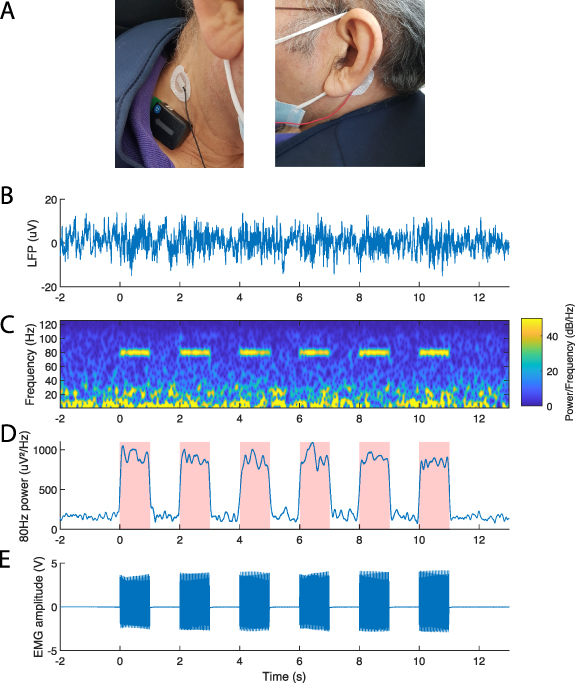
We managed to visualize the TENS artefact both on the LFP and EMG recordings in one patient with a DBS implant (figure 12) and in one patient with a cortical implant. Artefacts were successfully observed in the spectrograms of all six contact pairs (data not shown). The maximum difference between alignments was 12 ms (i.e. three LFP samples) in the DBS patient (figure 12) and 18 ms in the patient with ECoG leads. The artefact was evident when recording with Survey indefinite streaming modality with stimulation 'off' and can thus be used for synchronization instead of the DBS artefact. The TENS artefact cannot be monitored online, but was only evident after offline analysis.
Figure 12. Generation of a synchronization artefact with a transcutaneous electrical nerve stimulator (TENS) in a DBS patient. (A) Two surface electrodes (Neuroline 715, Ambu, Ballerup) were placed on the neck of patient CH5 over the lead extension and on the contralateral mastoid. An EMG probe (Trigno Avanti Sensor, Delsys) was placed on the neck. (B) Raw LFP signal recorded from 0 to 3 L in Survey indefinite streaming (stimulation 'off'). Note that the synchronization artefacts were not visible in the raw LFP signal. (C) Spectrogram displaying six 1 s TENS bursts (1 ms pulse width, 1.5 mA, charge-balanced square pulse, 80 Hz, interleaved with 1 s pause) recorded from 0 to 3 L, sent with an external stimulator. (D) Average power of the 78–82 Hz band with short-time Fourier transform at a 4 ms time resolution (200 ms window, 196 ms overlap) across all six contact pairs. Pink-shaded areas display the time-estimation of the stimulation artefacts. (E) The stimulation artefact was simultaneously recorded at 1259 Hz by the EMG probe.
Download figure:
Standard image High-resolution image
4. Discussion
The sensing capabilities of devices like Percept PC open new opportunities to optimize DBS clinical efficacy. First, the possibility of monitoring LFP power in chronically-implanted patients, both in-clinic and at home, allows readouts of symptom-specific brain activity patterns, their response to therapies, and fluctuations over time. These neurophysiological maps could complement anatomical model-based approaches for DBS programming, used to predict the shape of the volume of tissue activated [24, 25], to support informed stimulation programming. Second, real-time sensing algorithms provide the substrate for novel adaptive DBS systems that modulate stimulation parameters in response to an input signal representing symptoms, motor activity, or other behavioural features. These new protocols promise truly personalized treatment adherent to everyday life necessities, reducing side-effects and battery consumption, and overall improving therapeutic efficacy for a wider set of motor and non-motor symptoms.
Complementary to the clinical use, the sensing capacities offered by the Percept PC promise to foster translational and clinical research which, until recently, was limited to a few centres using externalized electrodes or who have access to research-dedicated devices [11, 26]. This represents an important springboard for extensive collaborations that aim to identify novel and more specific biomarkers and their true biological meaning.
4.1. Biomarkers identification
Our results confirm that the Percept PC is capable of recording and monitoring the most clinically-relevant biomarkers for PD and dystonia. In PD patients, a beta peak could be identified in at least one contact in 86% of STN (figures 1 and 3), suggesting that Streaming mode recordings could help clinicians to set the optimal stimulation amplitude for best beta-band power reduction (figure 1, supplementary figure 2).
The Percept PC also allows recording gamma-band modulations,Z opening opportunities for new symptom-specific and network-related biomarkers [27–29]. However, interpretations in this band need to be taken with caution, as the nature of modulations (either stimulation-related harmonics or artefacts) is unclear (figure 8). Similar stimulation-related signals were recorded earlier in patients implanted with the Activa PC+S [29]. The authors described them as an entrainment of the local gamma activity at half of the stimulation frequency in the presence of dyskinesia. In another study [30], the authors reported stimulation-induced subharmonics at half the stimulation frequency in 11/17 STN, which they interpreted as an electrical artefact. Similar to what we observed, the subharmonic artefacts had a narrow and stable frequency band, time-locked with stimulation, which supported their artefactual nature. Although these artefacts could interfere when monitoring high frequency content, the predictability of the artefact frequency and its features could help recognize them in post-processing phases. As a caveat, the relatively low sampling frequency (250 Hz) imposes some constraints to the computation of high-frequency oscillations [31].
Although the Percept PC is mainly intended for beta- and gamma-band recordings, a theta–alpha band was identified in 91% of non-artefactual contacts of dystonic patients, potentially offering a more meaningful approach for DBS programming in these patients.
4.2. Sensing options
The simplicity of manipulation and the signal quality of the Percept PC makes it an easy-to-use and reliable tool that can help guide the selection of optimal therapy parameters (e.g. stimulation contact pairs and amplitudes) during in-clinic visits, and monitor the condition of patients over longer periods at home and during daily activities. However, important aspects need to be considered to ensure reliable recordings. The most critical aspects were related to contact selection, artefact detection, and data loss.
The choice of the appropriate sensing mode is pivotal to how these aspects are handled by the device. Each mode provides specific pros and cons that make it more or less appropriate depending on the aim of the recording. For example, the Survey and Setup modes allow short recordings from all and stimulation-compatible contact pairs, respectively. They both check for the presence of artefacts, but only the latter performs this evaluation in simulation 'off' and 'on'. With the Streaming mode, sensing and stimulation contacts are restricted to predefined combinations that greatly reduce the available choices, but with the advantage of recordings of indefinite length simultaneous to active stimulation. To enable sensing, stimulation must be restricted to the middle contact points, which may not be the most clinically effective. In the near future, novel segmented electrodes might ease this issue. The Indefinite streaming mode allows recordings of indefinite length from all stimulation-compatible contact pairs, but data are not displayed in real time. Also, recordings in stimulation 'on' are not possible.
The Timeline mode provides the long-awaited possibility of chronically recording LFP; however recordings are restricted to the average power of a narrow band (5 Hz) around a predefined frequency. This selection remains static for the full extent of the recordings, and may therefore fail to capture modulations or frequency shifts [17]. Additionally, the possibility for patients to mark manually discrete events raises opportunities to obtain precise monitoring of specific symptom manifestations in real-life environments. While this may be indeed applicable for situations with slow-changing dynamics, such as on–off fluctuations, medication-induced dyskinesias, or sleep (figure 5), its utility for short episodic events such as freezing of gait or falls is less clear. Indeed, apart from heavily relying on patients compliance, the inevitable delay between the occurrence of the event and the manual marking with the patient controller, and the fact that only LFP after the marker are recorded would make it difficult to correlate the brain signal related to (the onset of) a short event. Furthermore, in Timeline mode the provided power averaged over 10 min would most likely miss short neural signatures related to these events [14]. These technical limitations significantly restrict the capacity to study such events, and would require the development of complementary solutions to deal with their episodic nature, such as the possibility of saving signals 'backward' from the marker.
4.3. Tips to identify and overcome artefacts and other issues
Based on our early experience, we summarized in table 2 some practical tips to identify and deal with technical issues that may arise both in clinical and experimental settings.
The Survey indefinite streaming is the only modality that allows continuous and indefinite LFP measurements with all contact pairs. However, the data streaming cannot be monitored online on the tablet or exported to third-party devices. This critically restricts any real-time application, and renders the correction or optimization of experimental setups inflexible. In this context, synchronization with other devices (e.g. EEG, EMG, etc) is an important issue also due to the inability to check a successful synchronization artefact online and the lack of an embedded synchronization method; this may represent a relevant limitation for research.
We also succeeded in synchronizing signals by means of a TENS artefact. The reliability of TENS synchronization needs to be confirmed in larger datasets. Indeed, the TENS artefact reproducibility and visualization may strongly depend on the characteristics of the TENS device and electrodes, and the stimulation protocol (i.e. amplitude, pulse width and frequency), which altogether warrant an optimization of the protocols on a single case basis.
The presence of various types of artefacts (i.e. cardiac, movement, and stimulation) was one of the major limitations in the use of this device. Specifically, the power band of cardiac artefacts overlaps with the beta frequency range and makes them particularly troublesome for proper monitoring of biomarkers, whether in-clinic or at home. It has been suggested that some surgical aspects (e.g. using two sutures to seal the connector between lead and extension or selecting the right implant site of the IPG [10, 32]) might influence the presence of artefacts, but results need to be confirmed as we could not find a consistent explanation in all our cases. Motion artefacts were also particularly challenging in dystonic patients, where episodic motor symptoms, such as myoclonic jerks, showed to impact the quality of the recordings to some extent. It is still unclear which aspects may influence the presence of motion artefacts. We could not identify any specific role of IPG location, impedance of the contacts, and stimulation conditions in this regard, but studies in larger cohorts might clarify these aspects. Given the episodic nature of these artefacts, longer recordings might be more robust for a proper evaluation of the frequency content of LFP signals in these patients. Of relevance, motion artefacts might be in some cases detectable only when observing the signals in correspondence of specific kinematic events (e.g. gait-related artefacts). The simultaneous use of devices for motion tracking (e.g. motion captures systems, inertial measurements units) when monitoring LFP during movement can help checking for the presence of motion artefacts.
It is important to note that although some LFP data and artefact information is available online and readily accessible through the user interface, more advanced analysis can only be performed offline. Data export is laborious and requires dedicated software; the exact time of saving the recording needs to be noted and files need to be monitored for data loss. To simplify this process, we provide an open-source code jointly with this report, which automatically extracts JSON files of the Percept PC and helps to account for missing data.
4.4. Conclusions
We hope that many of the above-mentioned drawbacks will soon be addressed and optimized. In the meantime, based on our initial multicentre experience in different clinical and research settings in patients with different diagnoses and in different conditions, we shared our practical tips to maximize the performance and signal quality of this novel device (table 2).
Sensing of LFP-based biomarkers will become routine in clinical practice, paving the way for better understanding and monitoring of distinctive neural signatures of specific symptoms or behaviours. However, a critical use of new technologies is warranted to identify and deal with possible shortcomings. This is a necessary premise for true patient-tailored neuromodulatory therapeutic interventions.
Acknowledgments
The authors would like to thank Professor C Matthies (UKW) for the neurosurgical information, Dr Henri Lorach (CHUV) for their help with data acquisition, and Dr Scott Stanslaski and Dr Gaetano Leogrande (Medtronic) for sharing some technical information on the system. Medtronic had no impact on the study design, data acquisition or writing of the manuscript. The draft manuscript was edited for English language by Deborah Nock (Medical WriteAway, Norwich, UK).
Data availability statement
The data generated and/or analysed during the current study are not publicly available for legal/ethical reasons but are available from the corresponding author on reasonable request.
Funding
C P and I U I were supported by the Deutsche Forschungsgemeinschaft (DFG, German Research Foundation)—Project-ID 424778381—TRR 295 and by the Fondazione Grigioni per il Morbo di Parkinson. E M and L B were supported by a grant from New York University School of Medicine and The Marlene and Paolo Fresco Institute for Parkinson's and Movement Disorders, which was made possible with support from Marlene and Paolo Fresco. Y T and E M M were funded by the Swiss National Science Foundation (Ambizione fellowship PZ00P3_180018), the Parkinson Schweiz foundation (Project OPTIM-GAIT) and the European Union H2020 program (Marie Sklodowska Curie Individual Action MSCA-IF-2017-793419) and the Gustaaf Hamburger funds of the Foundation Philantropia (Project 'Remarcher').
Credit authorship contribution statement
Y T: Conceptualization; Data curation; Formal analysis; Methodology; Software; Visualization; Writing—original draft. C P: Conceptualization; Data curation; Formal analysis; Methodology; Software; Visualization; Writing—original draft. A C: Formal analysis; Methodology; Writing—review and editing. B J K: Formal analysis; Software; Visualization; Writing—review and editing. P C: Data curation; Supervision; Writing—review and editing. M C J: Data curation; Writing—review and editing. J F B: Data curation; Writing—review and editing. E M: Data acquisition; Methodology; Writing—review and editing. L B: Data acquisition; Methodology; Writing—review and editing. R Z: Data curation; Supervision; Writing—review and editing. G C: Supervision; Resources; Writing—review and editing. J B: Data curation; Supervision; Writing—review and editing. N Avd G: Data curation; Supervision; Writing—review and editing. C F H: Data curation; Supervision; Writing—review and editing. E M M: Conceptualization; Data acquisition; Data curation; Formal analysis; Methodology; Resources; Supervision; Writing—original draft; Writing—review and editing. I U I: Conceptualization; Data acquisition; Data curation; Formal analysis; Methodology; Resources; Supervision; Writing—original draft; Writing—review and editing. M F C: Conceptualization; Data acquisition; Data curation; Formal analysis; Methodology; Resources; Supervision; Writing—original draft; Writing—review and editing.