
Abstract
Objective. Electroencephalography (EEG) cleaning has been a longstanding issue in the research community. In recent times, huge leaps have been made in the field, resulting in very promising techniques to address the issue. The most widespread ones rely on a family of mathematical methods known as blind source separation (BSS), ideally capable of separating artefactual signals from the brain originated ones. However, corruption of EEG data still remains a problem, especially in real life scenario where a mixture of artefact components affects the signal and thus correctly choosing the correct cleaning procedure can be non trivial. Our aim is here to evaluate and score the plethora of available BSS-based cleaning methods, providing an overview of their advantages and downsides and of their best field of application. Approach. To address this, we here first characterized and modeled different types of artefact, i.e. arising from muscular or blinking activity as well as from transcranial alternate current stimulation. We then tested and scored several BSS-based cleaning procedures on semi-synthetic datasets corrupted by the previously modeled noise sources. Finally, we built a lifelike dataset affected by many artefactual components. We tested an iterative multistep approach combining different BSS steps, aimed at sequentially removing each specific artefactual component. Main results. We did not find an overall best method, as different scenarios require different approaches. We therefore provided an overview of the performance in terms of both reconstruction accuracy and computational burden of each method in different use cases. Significance. Our work provides insightful guidelines for signal cleaning procedures in the EEG related field.
Export citation and abstract BibTeX RIS

Original content from this work may be used under the terms of the Creative Commons Attribution 4.0 license. Any further distribution of this work must maintain attribution to the author(s) and the title of the work, journal citation and DOI.
1. Introduction
Electroencephalography (EEG) allows to access brain activity and it is thus widely employed in a variety of clinical and research applications, including brain computer interfaces (Dornhege et al 2007), brain-controlled rehabilitation (Millán et al 2010, Luu et al 2017) and closed-loop neuromodulation (Schaworonkow et al 2019). The efficacy of such interventions is thus strongly affected by the quality of the EEG signal, which is by nature non-stationary and often includes a diverse set of artefacts. Indeed, EEG signals always present distortions due to environmental noise, e.g. power lines, or biological factors, such as eye-blinks, swallowing, clenching, and body movements in general (Libenson 2012). Moreover, a growing body of research is coupling EEG recordings with non invasive brain stimulation, either to guide stimulation (Dmochowski et al 2017) or to monitor its effects (Yavaria et al 2018). However, in the latter case, only the behavioral effects can be monitored during the application of the stimulation, while the EEG correlates are completely obscured by the stimulation artefact (Barban et al 2019). A crucial point in all EEG-related applications is thus the processing of raw data, which should lead to a clean and artefact-free signal, reliably reflecting the underlying brain oscillations (Jiang et al 2019). A wide adopted family of algorithms used to mitigate the effects of artefacts on the EEG signals belongs to blind source separation (BSS) techniques. These methods typically exploit diverse statistical properties of the EEG signal to linearly decompose it into some generative sources, assuming that signal corrupting artefacts are statistically independent from the desired neuronal signal, and therefore can be isolated and removed from the data (Jung et al 2000).
Biological artefacts arising from facial muscles and ocular movements have been extensively described, and different techniques for their removal have been proposed (Muthukumaraswamy 2013, Urigüen and Garcia-Zapirain 2015, Frø lich and Dowding 2018) and often distributed through open source pipelines available in the Web (Delorme and Makeig 2004, Oostenveld et al 2011).
EEG muscular contamination arises from the neck and face muscles, whose electrical activity is captured by the EEG sensors due to volume conduction (Whitham et al 2007). Facial muscles usually show a tonic activity, which leads to an ubiquitous contamination, even when the subject is at rest and relaxed (Goncharova et al 2003, Yilmaz et al 2019). Topologically, the artefact is usually more prominent in channels located most frontally, temporally or occipitally (Goncharova et al 2003). Moreover, the muscle groups that are majorly involved in the production of artefacts are also well known to have an electromyographic (EMG) activity overlapping the frequency bands of interest for EEG analysis (Whitham et al 2007). Specifically, frontalis and temporalis muscles can have peaks of activity in the [20–30] Hz band and in the [40–80] Hz band respectively (O'Donnell et al 1974, Goncharova et al 2003, Whitham et al 2007). For all these reasons, muscle artefacts have developed an infamous notoriety for being particularly hideous to deal with. Nevertheless, many artefact removal methods and strategies have been suggested over the years, with varying degrees of success, many of which rely on BSS techniques (Crespo et al 2008).
Ocular artefacts mainly arise from saccades and blinks and are usually detected as low frequency, high amplitude signal displacement (Libenson 2012). These artefacts are ubiquitous, easily recognizable, and can be effectively removed, because their amplitude is generally much larger than that of the background EEG activity (Jung et al 2000, Urigüen and Garcia-Zapirain 2015). In this case, decomposition methods based on morphology (Singh and Wagatsuma 2017) or in combinations with BSS (Lindsen and Bhattacharya 2010, Mahajan and Morshed 2015) are used. In many cases additional sources of signals, for example simultaneous recordings of electrooculogram (EOG) (Schlögl et al 2007) or eye movements (Noureddin et al 2012, Plöchl et al 2012, Mannan et al 2016) are also included.
The transcranial electrical stimulation (tES) artefact has recently risen to the community attention carried along with the gain in popularity that the corresponding neuromodulating techniques have enjoyed (Noury and Siegel 2017). The stimulation artefact has been characterized both on EEG and on magnetoencephalography and for different tES techniques: for transcranial alternating current stimulation (tACS) (Neuling et al 2017) as well as for transcranial direct current stimulation (Gebodh et al 2019). From these studies it emerged that the stimulation, especially when in its tACS declination, is not purely additive, but a modulation effect introduces a non-linearity in how the artefact is mixed with the signal. Moreover, this modulation is non-stationary since it also depends both on external biological or non-biological sources, and is therefore uncorrelated with the stimulation (Barban et al 2019). Thus, the resulting distortion of the ongoing oscillations makes artefact removal very challenging.
A few attempts have been recently made toward exploring techniques to remove, or at least reduce, the modulation artefact by post-processing the collected data (see (Kohli and Casson 2020) for a list). Most works focused on using template average subtraction (Kohli and Casson 2015), often in conjunction with other techniques, such as notch filters (Voss et al 2014), principal component analysis (PCA) (Helfrich et al 2014), and adaptive filtering (Kohli and Casson 2019). Other methods used are linear regression model subtraction (Schlegelmilch et al 2013) and regression coupled with BSS (typically independent vector analysis (IVA) or ICA) (Barban et al 2019, Lee et al 2019), some achieving even quasi real-time results (Guarnieri et al 2020).
In order to cope with the rich variety of available tools for signal denoising, which is often confusing and strongly related to the expertise of the operator, here we provide an overview of different methods and test their efficacy for EEG data cleaning. Starting from real EEG acquisition we first created semi-synthetic models of muscular, eye blink and tACS artefact. We then analyzed which tools are more suitable for removing the many artefactual components affecting the EEG traces, by performing denoising without any additional signals, e.g. without information derived by eye tracking devices, accelerometers, EOG and/or EMG recordings. We finally investigated a multi-step approach for serially removing tACS, eye blink and muscular artefacts from the recorded EEG.
2. Materials and methods
We tested a group of artefact removal techniques on different semi-synthetic datasets, each containing diverse sources of noise: muscular activity, eyeblinks or tACS artefacts.
2.1. Equipment and data collection
All the EEG data was collected using a high density EEG recording system (128 channels actiCHamp, Brain Products) at 1 kHz sampling rate from healthy adult individuals, with the approval of the institutional ethical committee. (CER Liguria reference 1293 of September 12, 2018). Four major data groups (table 1) were used during the study: one for each artefact model (muscular, eye blinks and tACS) and one clean group.
Table 1. Overview of the data used. Each artefact was derived from real world data, either appositely sampled for the study or gathered from available archives. We used the same equipment and parameters during all the acquisitions.
| Data type | # Subjects | Description |
|---|---|---|
| Clean | 26 | Resting state data from a set of experiments recorded in our Lab, visually inspected to find one consecutive minute of artefact-free activity. |
| Muscle | 5 | Ad hoc sampled data with stereotyped facial expressions to elicit muscular artefact (four subjects from our lab, 1 from Rantanen et al (2016)). |
| Blink | 41 | Resting and behaving data, coming from experiments acquired in our Lab. |
| tACS | 8 | Data containing tACS stimulation (40 Hz 675 µA), recorded in our Lab. |
Clean data was obtained using resting state recordings from 26 previous experiments, visually inspected by EEG expert users using freely available tools (i.e. EEGlab (Delorme and Makeig 2004), Brainstorm (Tadel et al 2011), and SPM (Baillet et al 2011)) to find one consecutive minute of artefact clean activity.
For the muscular artefact, we recorded EEG signals from four subjects for three 1 min long segments, during which they performed selected facial movements. The three segments were respectively dedicated to a frowning movement, a swallowing movement and a teeth clenching movement. In addition to the recorded EEG data, another facial EMG dataset was used to realistically model the artefact. These signals were obtained from a freely available online dataset (Rantanen et al 2016), which consists of facial surface EMG signals recorded from the corrugator supercilii, the zygomaticus major, the orbicularis oris, the orbicularis oculi, and the masseter muscles.
For the blink artefact, we did not sample any ad-hoc data, instead we used the many EEG datasets already available in the lab. These recordings also included two EOG channels that were used for the identification of blinks. In total 41 different datasets from various experiments and scenarios were used.
For the tACS data, we recorded from eight healthy subjects four different resting states sequences performed during stimulation, delivered using Brainstim (E.M.S. s.r.l., Italy). The stimulation parameters were: 675 µA (peak-to-peak) at 40 Hz, 325 µA at 40 Hz, 675 µA at 30 Hz and 325 µA at 30 Hz. These parameters were chosen according to Hoy et al (2015).
2.2. Artefact characterization
Our approach to the generation of realistic artefactual signals was heavily data driven. All the artefacts here described were created using snippets of biological signals, scaled and spatio-temporally distributed in a realistic manner, using maps derived from real artefact-corrupted EEG data. To highlight this feature, we refer to this model as semi-synthetic. This differs from what many studies do, where the artefactual traces are transposed into the EEG space using a projection matrix previously derived from another BSS method (Hoffmann and Falkenstein 2008), often without taking into account artefact topology (Chen et al 2014, 2018, Xu et al 2018). Instead, we built the artefactual model as independent from the tested algorithms as possible, in order to avoid any bias in the results.
2.2.1. Muscle artefact model generation
To recreate the muscular artefacts, we chose to embed EMG signals into an EEG trace, using realistic maps that reflected not only real data scaling but also the artefact topology. We derived these maps from appositely recorded EEG datasets: we acquired three segments of 1 min each from four subjects who were instructed to perform specific facial movements. The movements under scrutiny were frowning, swallowing and teeth clenching. The data acquired was then bandpass-filtered between 1 and 80 Hz and visually inspected to retrieve isolated artefact segments. Particular effort was put into finding segments of the signal where only one type of artefact was present, e.g. no simultaneous blink and muscular activity/movements. At least 10 s of signal for each facial expression were thus retrieved and used to map the power of the artefact throughout the sensor space. This measure was later normalized on the power of a clean resting state EEG acquired from the same subject during the same session. We will refer to this map as the 'power map'.
The same artefact-rich intervals were afterwards used to derive a 'correlation map' that we analyzed to determine the number of different muscular groups active during the inspected segments. This procedure worked as follows. For each facial expression and each subject we first computed a correlation matrix between the channels. The dimensionality of the matrix was then reduced using PCA, keeping the number of components explaining at least 80% of the variance. The reduced matrix was later clustered using a graph based technique described in Koontz et al (1976). As a result, we considered electrodes that clustered together as behaving in a similar manner and where therefore assigned to the same muscular unit. The number of these units determined the number of different EMG signals to be used in the generative model. All the clusters smaller than 5% of the number of electrodes were labeled as unclustered components, which received a white noise instead of an EMG signal. The selected components of the correlation matrix for each class were used to build an artefact projection matrix for each muscular unit, obtained by weighting each signal with its corresponding correlation score derived by the PCA reconstructed matrix. The procedure is schematized in figure 1.
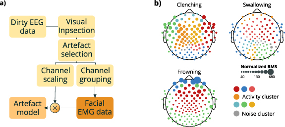
Figure 1. Muscular artefact generation. (a) Scheme of muscular artefact generation. Raw EEG data were first visually inspected (Visual inspection) to isolate at least 10 s of signals containing only one type of artefact (Artefact selection). These extracted artefact-rich segments were later used to derive both a scaling matrix and a correlation matrix, which were used respectively for channel scaling and channel grouping. The latter consisted in correlating signals among them, then to project the correlations in the PCA space, and finally clustering the group of signals into either muscular groups or residual unclustered components. After this step, each cluster was assigned an EMG signal (Facial EMG data). The projection into the EEG space was performed by weighting each of these EMG signals with its corresponding correlation score derived by the PCA reconstructed matrix. (b) Representation of geometrical distribution across the scalp of unclustered components (grey dots) and signal clusters (colored dots) of typical subjects. Dots' size encodes the signal intensity, computed as the channel's RMS level normalized over the RMS level of its corresponding resting state activity.
Download figure:
Standard image High-resolution image2.2.2. Blink artefact model generation
To model the blink artefact, we chose a completely data driven approach. Using 41 different datasets, we built a blinking dictionary that was later used to create a plausible artefact model. The EOG channels of each dataset were selected and low pass filtered at 7 Hz to isolate the blinking waveform, whose power spectrum is concentrated at the low frequencies (Libenson 2012). Afterwards, we performed a very simple blink detection by selecting local maxima greater than two times the standard deviation of the inspected channel (using findpeaks function in MATLAB). We noticed that some subjects have a tendency to quickly blink many times in a row. Therefore, in order to avoid selecting multiple blinks many times, we pruned our collection by removing those peaks that did not display a zero crossing with at least half a second delay between them. We stored the timestamp (ts) of the blink, as well as 1 s long snippet around it (ts − 500 ms, ts + 500 ms). An amplitude map was then built by sampling, for each EEG channel, the amplitude value at the peak of each blink and averaging this value across all the events.
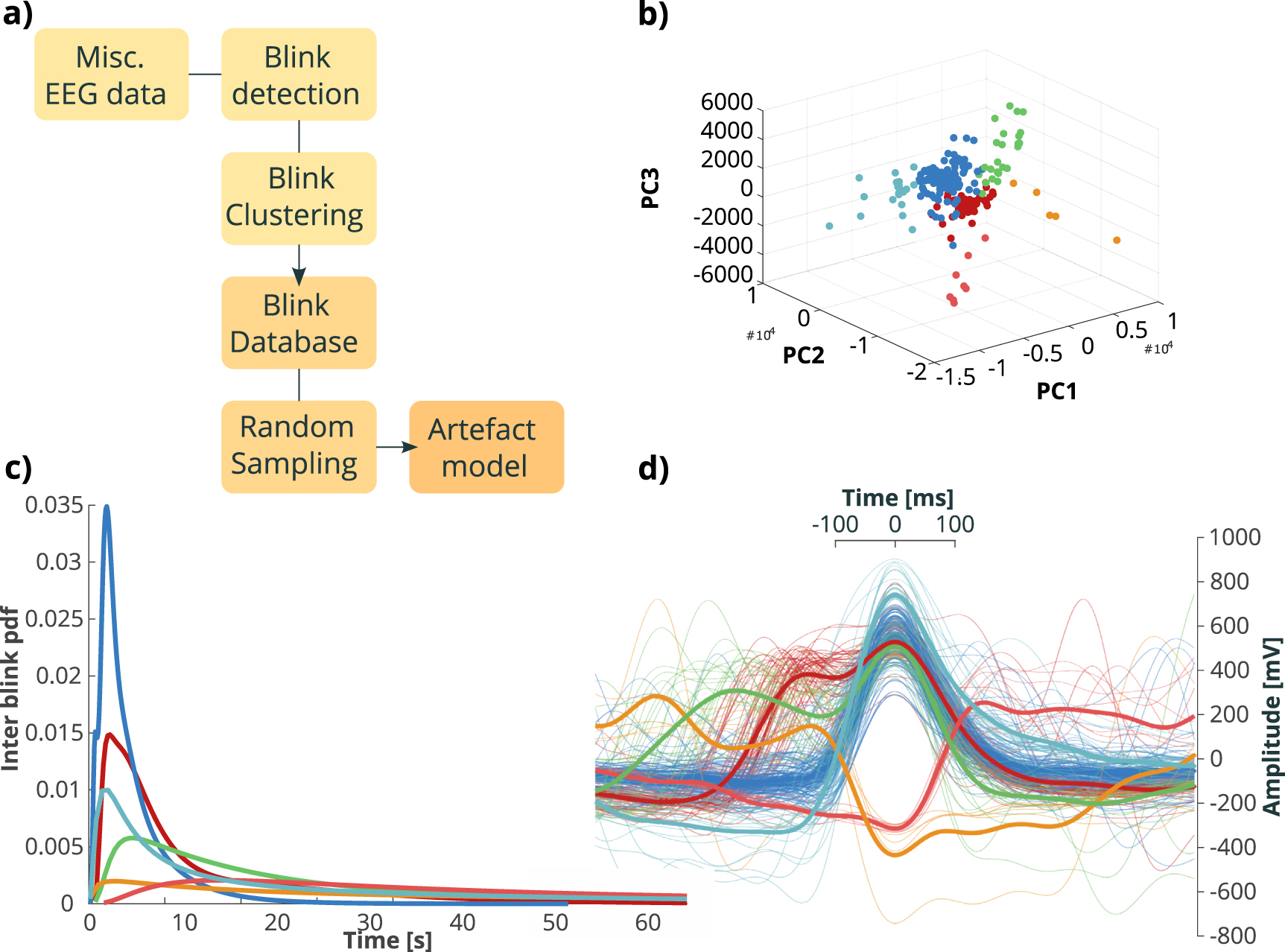
We then performed a clustering procedure, separately for each subject, in order to retrieve prototype blinking waveforms. For each prototype we also derived a inter event probability distribution. A blinking point process was derived by resampling the associated distribution. Afterwards, we placed at each ts one random waveform chosen between those stored in the dictionary. 21 semi-synthetic artefacts traces were thus created. The procedure is schematized in figure 2.
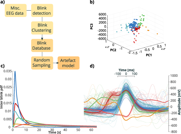
Figure 2. Blink artefact generation. (a) Scheme of blink artefact generation. EEG data first underwent a blink detection procedure. Blinks were then clustered with K-means algorithm applied to PCA projected data. A blink database was thus built and probability density functions of each prototype were used to randomly sample waveforms to create artefact models. (b) Waveforms of panel (d) represented in space of the first three components extracted with PCA. (c) Inter Blink probability density functions of clusters of data presented in (b). (d) Different blinking waveforms of one typical subject, colored according to clusters. Thick lines represent average cluster waveforms.
Download figure:
Standard image High-resolution image2.2.3. tACS artefact model generation
tACS artefact suffers from some unique characteristics which make its removal particularly tricky. This has to be taken into account while building a proper model. Unlike the previous simulations, in fact, it cannot be simply modeled as a linear addition to the signal, because both biological and non biological factors exert a modulation effect on the stimulation current (Barban et al 2019). Moreover, it has been shown how these modulation factors occur independently from the stimulation frequency (Noury et al 2016). To isolate the stimulation artefact and preserve its nonlinear and non-stationary nature, we first bandpass-filtered the eight acquisitions containing the artefact; the limits of the filter were chosen depending on the value of the stimulation frequency minus (lower limit) or plus (upper limit) 10 Hz. Afterwards, we obtained the slow changing envelope that amplitude modulates the sinusoidal stimulus in the raw data, by taking the magnitude of its corresponding analytic signal. For each channel, a numerically generated sine wave was multiplied with its corresponding envelope, to create a realistic model of the artefact. To cover the whole EEG spectrum, we chose to test three frequencies peculiar of alpha, low gamma and high gamma band: 10, 40 and 60 Hz. The procedure is schematized in figure 3.

Figure 3. tACS artefact generation. (a) Scheme of tACS artefact generation. Artefactual EEG acquisitions (Stim. Data) were bandpass filtered (Isolated Artefact) to isolate the slow changing envelopes (Envelope) modulating the tACS artefact. Afterwards, these were multiplied by a numerically generated sine wave to obtain many artefact models at different carrier frequencies (10, 40 and 60 Hz). (b) 40 Hz tACS artefact in time domain (blue trace, downscaled by a factor of 103). An artefact attenuation step, in the form of subtraction of the sinusoidal best fit, was performed to highlight the induced nonlinear modulation effect captured by the model. The difference with the original clean data (yellow) is displayed in green. (c) 40 Hz tACS artefact in frequency domain. The frequency spectrum of the artefact was obtained with multitaper power spectral density (pmtm function in MATLAB). A leftover effect due to the modulation is visible at the reduced peak around 40 Hz.
Download figure:
Standard image High-resolution image2.3. Data generation
By linearly combining the clean data with an artefact model, a semi-synthetic dataset was created. A normalization factor was obtained from the power of the signals used to model the artefacts. During the generative step, all the artefact models were normalized using the corresponding factors. In this way it was possible to match the amplitude of the artefact to the amplitude of the clean dataset used as ground truth. This was done in order to create a realistic signal to noise ratio (SNR) distribution. SNR was defined as follows:
with N being the total number of channels and T the total number of samples contained in the signal X.
A brief schematic of this step is available in figure 4.
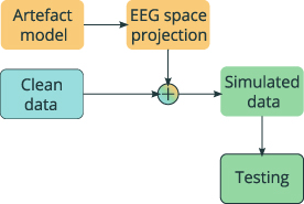
Figure 4. Scheme of data generation procedure. For each artefact type, the corresponding model (Artefact model) was projected in the EEG space using previously obtained projection matrices (EEG space projection). By linearly combining it with a ground truth signal (Clean data) a semi-synthetic dataset (Simulated data) was obtained and used for algorithm evaluation (Testing).
Download figure:
Standard image High-resolution imageThe nature and the total number of datasets generated is summarized in table 2. The data generated this way is freely available online (Barban et al 2021). The number of the actually used datasets ended up being lower than the theoretical maximum, in order to keep the testing time reasonable. Finally, randomly picked samples from the three different datasets' groups were linearly mixed to obtain a lifelike testing set containing multiple noise sources.
Table 2. Overview of the semi-synthetic data used in the study. Here are reported the number of artefactual snippets and clean data used to generate the testing datasets and the number of datasets generated for this study. The theoretical maximum number of test datasets achievable this way (Artefactual snippets * Clean segments) is also reported in brackets. Only a subset of this maximum was here used due to the computational burden.
| Dataset type | Artefactual snippets | Clean data available | Datasets generated (Theoretical maximum) |
|---|---|---|---|
| Muscolar | 90 | 26 | 610 (2340) |
| tACS | 20 | 26 | 360 (520) |
| Blink | 21 | 26 | 210 (546) |
| Mixed | 37 800 | 26 | 600 (982 800) |
2.4. Testing platform
We tested different cleaning strategies on the semi-synthetic data. For each artefact type, we generated many different datasets that were later used to test various cleaning techniques. The testing procedure was automatized and did not required any human interaction: after the BSS step performed with the algorithms specified below, the obtained independent components (ICs) were ordered based on their correlation (with the original known artefact. Afterwards, we iteratively removed an increasing number of ICs until the correlation with the clean datasets started to drop. This meant that the best trade-off between artefactual and brain content had been reached.
2.4.1. Algorithms tested and cleaning procedure
We tested different BSS algorithms: canonical correlation analysis (CCA) (Hotelling 1992, Borga 2001); Independent Component Analysis in its fastICA implementation (Hyvärinen and Oja 2000), both in the deflation (fastICA defl) and symmetric (fastICA symm) variant, and in its Infomax implementation (infomax) (Bell and Sejnowski 1995); IVA (Chen et al 2017) using a quasi-Newton optimization approach for speed purposes as in Anderson et al (2011). Differently from ICA based algorithms, for CCA and IVA we first needed to shape our data as to make them suitable for these methods. CCA and IVA were conceived for joint BSS problems, which are characterized by the need to solve many individual BSS simultaneously by assuming statistical dependence between latent sources across datasets (Lahat and Jutten 2014). To reshape our datasets in order to fit into this category, we created several copies of the same dataset, shifting each copy of a fixed amount of temporal samples, corresponding to 8 ms.
Each algorithm was tested with and without a prior PCA based dimensionality reduction step. Indeed, this operation can be performed before a BSS step in order to speed up its execution. We chose the number of principal components (PCs) included in subsequent computations by thresholding on the 95th percent of the explained variance.
An ad hoc filtering step was performed before the BSS step for the blink and muscular artefacts, in a subset of the tested algorithms, namely CCA, fastICA symm and IVA. The rationale behind this choice was to limit the amount of the brain originated signal in the removed ICs, thus highlighting the contribution of the noisy components. The filter here used was a zero lag infinite impulse response filter with a stopband frequency of 8 Hz. Given the spectral distribution of muscular and blink artefacts (Urigüen and Garcia-Zapirain 2015), the filter was respectively implemented as highpass and lowpass.
IVA was also tested in two different parameterizations. The first one with the weights randomly initialized and five temporal shifts in the dataset and the second one preinitialized using CCA and with only two shifts (IVA fast). Table 3 lists the utilized algorithms and the different implementations used to run them.
Table 3. Algorithms used in the study. When  is present, the algorithm was tested both with and without the indicated preprocessing step. 'PCA' denotes a PCA-based dimensionality reduction step, while 'Filter' denotes a focal filtering step used to reduce the amount of brain related content in the signal prior to the BSS step.
| Algorithm | PCA | Filter | Reference |
|---|---|---|---|
| CCA |

|

| (Hotelling 1992, Borga 2001) |
| fastICA defl |

| (Hyvärinen and Oja 2000) | |
| fastICA symm |

|

| (Hyvärinen and Oja 2000) |
| infomax |

| (Bell and Sejnowski 1995) | |
| IVA |

|

| (Anderson et al 2011) |
| (Chen et al 2017) |
2.4.2. Multi-step Artefact reduction
After the identification of the best performing algorithm for each type of artefact, we explored a multi-step procedure to progressively remove artefacts of different nature from the same trace. The procedure started with the removal of the tACS artefacts, followed by reduction of biological artefacts. We compared this procedure with a single-step approach, where the dirty EEG signal was cleaned in a single iteration.
We tested the multi-step approach with different combinations of algorithms, i.e. by using the same algorithm three times in a row or by using different methods for each step. For example in a trial we used the best performing algorithm for removal of tACS artefact (tACS_top) to remove all the three artefactual sources, in another trial the best eye-blink cleaner (blink_top) was used and in another one the best muscular suppressor (muscle_top);
We also performed the multi-step procedure, but this time using for each artefact the best performing method for its removal: i.e. tACS_top for removing the tACS artefact, followed by the application of blink_top for eye-blink and muscle_top for muscular derived artefact.
The single step procedure was implemented in three tests, each using one of the best performing algorithms for each type of artefact (i.e. tACS_top or blink_top or muscle_top).
Table 4 summarized the various combinations of algorithms used in the tests run for implementing the multi and single-step procedure.
Table 4. Multi-step procedure implementations. Each column indicates the algorithms used for cleaning each artefact in a given test.
| Artefact | Test 1 | Test 2 | Test 3 | Test 4 | |
|---|---|---|---|---|---|
| Multi-step | tACS | tACS_top | blink_top | muscle_top | tACS_top |
| blink | tACS_top | blink_top | muscle_top | blink_top | |
| muscular | tACS_top | blink_top | muscle_top | muscle_top | |
| Single-step | all | tACS_best | blink_best | muscle_best |
2.4.3. Metrics for evaluation of algorithms performance
We evaluated performance of the different procedures in terms of similarity between the cleaned and original dataset, and also in terms of computational time.
We assessed dataset similarity with cosine similarity measure (CSM) and with the relative root mean square error (RRMSE).
CSM is defined as:
where N is the number of EEG channels, EEGC is the clean EEG signal and EEGR is the reconstructed one, both of duration T.
RRMSE is defined as:
with RMS defined as in equation (2).
Computational times for the BSS step were also collected, without taking into account any preliminary steps such as PCA-based dimensionality reduction, filtering or sinusoidal best fit subtraction(tACS only). All the testing was performed in MATLAB 2019b on a machine configured with an Intel Xeon E5-2630 CPU clocked at 2.40 GHz and 32 GB of system memory running at 2133 MHz.
Statistical comparisons among scores obtained by different algorithms were performed using the Kruskal–Wallis method implemented in MATLAB 2019b and the statistical significance level was set to p < 0.05.
3. Results
Different semi-synthetic EEG datasets were created by modeling three types of artefacts: muscular, blinking and tACS. These datasets were used to test several artefact removal approaches, based on some of the most popular BSS techniques (ICA, IVA, CCA). We evaluated the cleaning ability of BSS algorithms by comparing the cleaned data with the available ground truth. The metrics used for this comparison were: CSM, RRMSE and computational time.
Results are separately reported for each artefactual type and are organized as follows. Median and interquartile range of CSM and RRMSE scores, as well as computational time obtained by each algorithm are reported in dedicated tables (tables 5–8).
Table 5. Removal of muscular artefact. Here are reported (median and interquartile range) the values of the reconstruction quality metrics used in the study (CSM,RRMSE), together with the correlation coefficient ρ between the two. High values of ρ reflect a linear trend between the metrics. The computational time is also reported.
| CSM | RRMSE | Comp. time (s) | |||||
|---|---|---|---|---|---|---|---|
| Algorithm | Median | IQR | Median | IQR | Median | IQR | ρ |
| CCA, PCA + filter | 0.88 | 0.82–0.9 | 0.56 | 0.49–0.71 | 14.66 | 12.41–22.43 | −0.94 |
| CCA, PCA | 0.92 | 0.89–0.94 | 0.43 | 0.35–0.5 | 15.57 | 12.24–19.74 | −0.96 |
| CCA, filter | 0.81 | 0.77–0.89 | 0.78 | 0.57–1.05 | 64.5 | 41.65–68.56 | −0.96 |
| CCA | 0.9 | 0.87–0.93 | 0.47 | 0.38–0.55 | 57.4 | 38.63–66.57 | −0.96 |
| fastICA defl, PCA | 0.91 | 0.86–0.96 | 0.48 | 0.3–0.65 | 68.38 | 38.53–132.85 | −0.99 |
| fastICA defl | 0.89 | 0.83–0.95 | 0.54 | 0.35–0.75 | 219.69 | 173.19–296.58 | −0.99 |
| fastICA symm, PCA + filter | 0.99 | 0.97–0.99 | 0.16 | 0.12–0.23 | 68.37 | 44.03–94.85 | −0.98 |
| fastICA symm, PCA | 0.99 | 0.98–1 | 0.13 | 0.09–0.19 | 103.53 | 65.54–142.02 | −0.97 |
| fastICA symm, filter | 0.89 | 0.77–0.98 | 0.57 | 0.19–1.05 | 194 | 170.44–209.81 | −0.99 |
| fastICA symm | 0.99 | 0.97–1 | 0.14 | 0.08–0.23 | 201.17 | 183.77–231.28 | −0.97 |
| infomax, PCA | 0.94 | 0.91–0.95 | 0.36 | 0.31–0.43 | 398.87 | 301.75–601.3 | −0.98 |
| infomax | 0.92 | 0.88–0.94 | 0.43 | 0.35–0.58 | 154.34 | 50.68–254.05 | −0.98 |
| IVA fast, PCA | 0.92 | 0.89–0.94 | 0.42 | 0.35–0.5 | 14.94 | 11.64–19.65 | −0.96 |
| IVA fast | 0.88 | 0.77–0.92 | 0.53 | 0.43–0.89 | 29.21 | 27.75–30.86 | −0.86 |
| IVA, PCA + filter | 0.95 | 0.92–0.97 | 0.31 | 0.26–0.42 | 65.34 | 36.58–294.36 | −0.98 |
| IVA, PCA | 0.98 | 0.97–0.99 | 0.2 | 0.16–0.26 | 112.58 | 61.58–270.57 | −0.97 |
| IVA, filter | 0.79 | 0.77–0.89 | 0.91 | 0.57–1.11 | 623.62 | 540.25–782.49 | −0.79 |
| IVA | 0.96 | 0.86–0.98 | 0.27 | 0.22–0.64 | 1880.28 | 1833.34–1986.58 | −0.92 |
Both the CSM and RRMSE scores are graphically presented as violin plots for each algorithm used (panels (a) for CSM and (b) for RRMSE in figures 5–8). We then selected the two best performing algorithms as those obtaining the highest and statistically distinguishable scores both for CSM and RRMSE. For these algorithms, a direct comparison is also reported (panels (c) for CSM and (e) for RRMSE in figures 5–8), with superimposed a scatterplot relating the scores with the SNR of the dataset. The SNR distribution is also reported on the x-axis. Note that the CSM and RRMSE violin plots only provide information on the density of the points in the scatterplot and must not be directly related to the SNR distribution (x-axis).
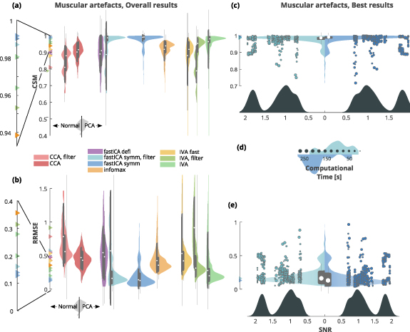
Figure 5. Removal of muscular artefact. (a) CSM scores obtained by the used algorithms (higher is better). Algorithms performance is depicted as paired violins plot, where left/right distribution indicate algorithm performance without/with previous PCA step. Each algorithm is depicted in a different color and superimposed in grey is a boxplot describing the median value (white dot), 25th and 75th percentiles (extremes of the thick grey line), and full data range (extremes of the thin grey line). (b) RRMSE scores obtained by the used algorithms (lower is better). Color code same as in (a). (c) CMS violin plot of the two best performing algorithms: symmetric fastICA with and without previous filtering, both with a PCA-based dimensionality reduction step. The full scatterplot is superimposed (CSM against SNR) and the points size indicates the computational time required by the method. Legend of computational time is reported in (d). Color code same as in (a). (d) Computational time legend (seconds) with superimposed its distribution for best performing algorithms. Color code same as in (a). (e) RRMSE violin plot of the two best performing algorithms: symmetric fastICA with and without filtering, both with a PCA-based dimensionality reduction step. The full scatterplot is superimposed (RRMSE against SNR) and the points size indicates the computational time required by the method. Legend of computational time is reported in (d). Color code same as in (a).
Download figure:
Standard image High-resolution imageThe computational time is graphically reported for the two best performing algorithms and is encoded as the dimension of the points in the scatterplot. A legend is provided (panel (d) in figures 5–8) with an additional distribution for improved clarity.
The supplementary material section contains visual representation of the outcome of the Kruskal–Wallis tests for the CSM and RRMSE scores.
Scatterplots highlighting the correlation between: (a) CMS and RRMSE scores, (b) CSM score and SNR, (c) computational time and CSM score, and (d) computational time and SNR are also reported in the supplementary material section, for the best performing algorithm only.
3.1. Muscular artefact removal
Both CSM and RRMSE revealed that removal of muscular artefact was most successful when using symmetric fastICA with and without a PCA based dimensionality reduction step. For both metrics the median results are almost the same (CSM: 0.99 and 0.99; RRMSE: 0.14 and 0.13 for fastICA without and with PCA respectively, table 5). Moreover, good results were also reached with a preemptive filtering step, but only when coupled with a PCA based dimensionality reduction step (CSM: 0.99; RRMSE: 0.16, table 5). Lastly, also IVA showed good performance when preceded by PCA (CSM: 0.98; RRMSE: 0.2, table 5). Between these four best performing algorithms, the top three (fastICA based) showed no statistical differences in CSM and RRMSE scores among them, while IVA differed only from the very top performer (symmetric fastICA with previous PCA, supplementary figures 9 and 10 (is available online at stacks.iop.org/JNE/18/0460c2/mmedia)). We thus selected, for an in depth comparison, the symmetric fastICA and the fastICA algorithm with the previous filtering, both with previous PCA.
Figure 5 shows an overview of the results, as described at the beginning of the Results section.
We observed that CSM and RRMSE have the same trend and linearly covariate with a correlation of ρ, in module, higher than 0.9 in most methods, with the exception of some IVA-based algorithms, for which it drops up to 0.79 (see table 5 as well as supplementary figures 1 and 2).
The computational time required for algorithm execution was also tracked (figure 5 panels (b) and (d) and table 5). We did not observe any link between computational time and CSM, RRMSE, or SNR as shown in supplementary figures 1 and 2 which report the relation between CSM, RRMSE and computational time for the best performing methods.
We also generally noticed that a high-pass filtering step performed prior to the application of the BSS method, was slightly detrimental to the overall reconstruction performance: decreasing the reconstruction score while also increasing its dispersion. The rationale behind this pre-filtering step, is to preserve the frequency content mostly associated with the EEG signal, while suppressing the artefact in higher frequencies.
On the other hand, the dimensionality reduction step based on PCA, generally improved the distribution of results, both in terms of median values and dispersion of the data.
3.2. Blink artefact removal
Both CSM (figure 6 panel (a)) and RRMSE (figure 6 panel (b)) appoint IVA as the best performing algorithm to correct for blinking (CSM: 1; RRMSE: 0.07, table 6), directly followed by CCA, then fastICA in its symmetric version, and IVA in its fast implementation (CSM: 1 for all these algorithms, RRMSE: 0.08 for CCA, 0.1 for fastICA and IVA fast, table 6). None of these top performing algorithms resulted to be statistically different from the other three, neither according to CSM nor to RRMSE (supplementary figures 9 and 10). It is worth noticing that the best algorithms did not involve PCA dimensionality reduction, as it always resulted in worse performance.
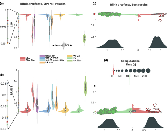
Figure 6. Removal of blink artefact. (a) CSM scores obtained by the used algorithms (higher is better). Algorithms performance is depicted as paired violins plot, where left/right distribution indicate algorithm performance without/with previous PCA step. Each algorithm is depicted in a different color and superimposed in grey is a boxplot describing the median value (white dot), 25th and 75th percentiles (extremes of the thick grey line), and full data range (extremes of the thin grey line). (b) RRMSE scores obtained by the used algorithms (lower is better). Color code same as in (a). (c) CMS violin plot of the two best performing algorithms: IVA and CCA. The full scatterplot is superimposed (CSM against SNR) and the points size indicates the computational time required by the method. Legend for computational time is reported in (d). Color code same as in (a). (d) Computational time legend (seconds) with superimposed its distribution for best performing algorithms. Color code same as in (a). (e) RRMSE violin plot of the two best performing algorithms: IVA and CCA. The full scatterplot is superimposed (RRMSE against SNR) and the points size indicates the computational time required by the method. Legend for computational time is reported in (d). Color code same as in (a).
Download figure:
Standard image High-resolution imageTable 6. Removal of blinking artefact. Here are reported (median and interquartile range) the values of the reconstruction quality metrics used in the study (CSM,RRMSE), together with the coefficient of determination R2 for a linear regression between the two. High values of R2 reflect a linear trend between the metrics. The computational time is also reported.
| CSM | RRMSE | Comp. time (s) | |||||
|---|---|---|---|---|---|---|---|
| Algorithm | Median | IQR | Median | IQR | Median | IQR | ρ |
| CCA, PCA + filter | 0.88 | 0.85–0.91 | 0.61 | 0.51–0.73 | 4.56 | 4.28–5.87 | −0.83 |
| CCA, PCA | 0.99 | 0.98–0.99 | 0.18 | 0.12–0.27 | 14.7 | 9.51–19.81 | −0.77 |
| CCA, filter | 0.8 | 0.78–0.83 | 1.07 | 0.95–1.2 | 41.72 | 26.69–55.8 | −0.54 |
| CCA | 1 | 0.99–1 | 0.08 | 0.06–0.14 | 43.87 | 23.1–56.7 | −0.91 |
| fastICA defl, PCA | 0.96 | 0.89–0.98 | 0.36 | 0.22–0.68 | 29.1 | 14.07–126.69 | −0.97 |
| fastICA defl | 0.93 | 0.91–0.97 | 0.42 | 0.27–0.62 | 147.5 | 122.78–201.96 | −0.95 |
| fastICA symm, PCA + filter | 0.96 | 0.93–0.97 | 0.38 | 0.28–0.56 | 5.18 | 4.67–7.42 | −0.96 |
| fastICA symm, PCA | 0.98 | 0.96–0.99 | 0.25 | 0.17–0.36 | 34.53 | 17.06–128.11 | −0.95 |
| fastICA symm, filter | 0.85 | 0.82–0.89 | 0.84 | 0.66–1.02 | 47.05 | 36.47–59.91 | −0.84 |
| fastICA symm | 1 | 0.99–1 | 0.1 | 0.07–0.14 | 156.29 | 135.25–176.23 | −0.89 |
| infomax, PCA | 0.94 | 0.91–0.96 | 0.45 | 0.31–0.74 | 317.22 | 194.6–605.61 | −0.88 |
| infomax | 0.93 | 0.89–0.95 | 0.51 | 0.36–0.81 | 227.98 | 210.44–239.72 | −0.89 |
| IVA fast, PCA | 0.99 | 0.98–0.99 | 0.18 | 0.12–0.28 | 14.84 | 9.52–20.2 | −0.77 |
| IVA fast | 1 | 0.99–1 | 0.1 | 0.07–0.18 | 20.41 | 19.6–23.62 | −0.91 |
| IVA, PCA + filter | 0.78 | 0.77–0.8 | 1.16 | 1.02–1.36 | 5.64 | 5.01–6.33 | −0.68 |
| IVA, PCA | 0.99 | 0.99–0.99 | 0.15 | 0.11–0.23 | 127.92 | 32.77–324.86 | −0.9 |
| IVA, filter | 0.78 | 0.77–0.8 | 1.17 | 1.03–1.38 | 751.93 | 500.05–1447.34 | −0.67 |
| IVA | 1 | 1–1 | 0.07 | 0.04–0.1 | 2352.8 | 2331.31–2375.31 | −0.9 |
For the majority of the tested algorithms, a strong correlation was found between CSM and RRMSE scores (table 6).
We also generally observed that a low-pass filtering step performed prior to the application of the BSS methods, was clearly detrimental to the overall reconstruction performance.
We selected for an in depth comparison IVA and CCA algorithms, both without filtering and previous PCA (figure 6 panels (c) and (e), as described at the beginning of the Results section.)
The full distribution of the computational times is available in figure 6 panel (d), where it emerges that, despite having very comparable reconstruction results, CCA is clearly advantageous in terms of computational resources.
Correlations between performance (i.e. CSM and RRMSE) and computational time as well as between performance and SNR, were very low, if not absent, for the top performing algorithms, as shown in supplementary figures 3 and 4.
3.3. tACS artefact removal
Both CSM and RRMSE revealed that removal of tacs artefact was most successful when using IVA without a PCA based dimensionality reduction step, followed by IVA with previous PCA. For both metrics the median results are almost the same (CSM: 0.966 and 0.958; RRMSE: 0.26 and 0.28 for IVA without and with PCA respectively, table 7). Moreover, good results were also reached with symmetric fastICA, with and without previous PCA (CSM: 0.949 and 0.946; RRMSE: 0.322 and 0.324 for fastICA without and with PCA respectively, table 7). Panels a and b of figure 7 show an overview of the results, depicting for each method the distribution across the datasets of the reconstruction scores.
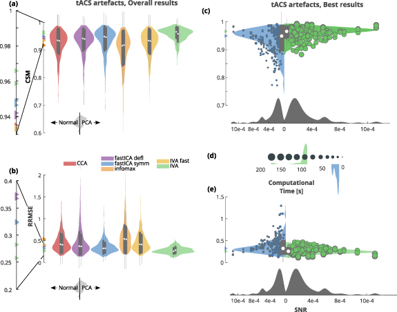
Figure 7. Removal of tACS artefact. (a) CSM scores obtained by the used algorithms (higher is better). Algorithms performance is depicted as paired violins plot, where left/right distribution indicate algorithm performance without/with previous PCA step. Each algorithm is depicted in a different color and superimposed in grey is a boxplot describing the median value (white dot), 25th and 75th percentiles (extremes of the thick grey line), and full data range (extremes of the thin grey line). (b) RRMSE scores obtained by the used algorithms (lower is better). Color code same as in (a). (c) CMS violin plot of the two best performing algorithms: symmetric fastICA and IVA, both without a PCA-based dimensionality reduction step. The full scatterplot is superimposed (CSM against SNR) and the points size indicates the computational time required by the method. Legend of computational time is reported in (d). Color code same as in (a). (d) Computational time legend (seconds) with superimposed its distribution for best performing algorithms. Color code same as in (a). (e) RRMSE violin plot of the two best performing algorithms: symmetric fastICA and IVA, both without a PCA-based dimensionality reduction step. The full scatterplot is superimposed (RRMSE against SNR) and the points size indicates the computational time required by the method. Legend of computational time is reported in (d). Color code same as in (a).
Download figure:
Standard image High-resolution image
Figure 8. Removal of mixed artefact. (a) CSM scores obtained by the used algorithms (higher is better). Algorithms performance is depicted as paired violins plot, where left/right distribution indicate algorithm performance without/with previous PCA step. Each algorithm is depicted in a different color and superimposed in grey is a boxplot describing the median value (white dot), 25th and 75th percentiles (extremes of the thick grey line), and full data range (extremes of the thin grey line). (b) RRMSE scores obtained by the used algorithms (lower is better). Color code same as in (a). (c) CMS violin plot of the two best performing algorithms: multistep IVA with PCA-based dimensionality reduction step and multi 2 (i.e. IVA + CCA + fastICA, PCA). The full scatterplot is superimposed (CSM against random jitter for the sake of visualization) and the points size indicates the computational time required by the methods. Legend of computational time is reported in (d). Color code same as in (a). (d) Computational time legend (seconds) with superimposed its distribution for best performing algorithms. Color code same as in (a). (e) RRMSE violin plot of the two best performing algorithms: multistep IVA with PCA-based dimensionality reduction step and multi 2 (i.e. IVA + CCA + fastICA, PCA). The full scatterplot is superimposed (CSM against random jitter for the sake of visualization) and the points size indicates the computational time required by the method. Legend of computational time is reported in (d). Color code same as in (a).
Download figure:
Standard image High-resolution image
Table 7. Removal of tACS artefact. Here are reported (median and interquartile range) the values of the reconstruction quality metrics used in the study (CSM,RRMSE), together with the correlation coefficient ρ between the two. High values of ρ reflect a linear trend between the metrics. The computational time is also reported.
| CSM | RRMSE | Comp. time (s) | |||||
|---|---|---|---|---|---|---|---|
| Algorithm | Median | IQR | Median | IQR | Median | IQR | ρ |
| CCA, PCA | 0.93 | 0.91–0.95 | 0.4 | 0.32–0.55 | 23.08 | 19.93–26.05 | −0.75 |
| CCA | 0.93 | 0.91–0.96 | 0.41 | 0.32–0.56 | 23.2 | 21.7–25.12 | −0.71 |
| fastICA defl, PCA | 0.94 | 0.92–0.96 | 0.37 | 0.28–0.53 | 69.69 | 46.11–100.03 | −0.59 |
| fastICA defl | 0.94 | 0.92–0.96 | 0.37 | 0.29–0.58 | 164.12 | 134–201.78 | −0.64 |
| fastICA symm, PCA | 0.95 | 0.92–0.96 | 0.32 | 0.27–0.4 | 46.03 | 35.76–80.27 | −0.95 |
| fastICA symm | 0.95 | 0.92–0.97 | 0.32 | 0.26–0.43 | 75.52 | 56.39–127.64 | −0.85 |
| infomax, PCA | 0.92 | 0.88–0.94 | 0.53 | 0.35–0.68 | 446.58 | 326.82–589.09 | −0.61 |
| infomax | 0.92 | 0.87–0.94 | 0.54 | 0.36–0.7 | 219.23 | 202.94–232.35 | −0.63 |
| IVA fast, PCA | 0.93 | 0.91–0.95 | 0.41 | 0.32–0.55 | 23.2 | 20.03–26.42 | −0.75 |
| IVA fast | 0.93 | 0.91–0.96 | 0.41 | 0.32–0.57 | 29.11 | 26.13–31.91 | −0.71 |
| IVA, PCA | 0.96 | 0.94–0.97 | 0.28 | 0.24–0.33 | 206.39 | 109.07–336.82 | −0.97 |
| IVA | 0.97 | 0.95–0.97 | 0.26 | 0.22–0.31 | 1808.13 | 1775.7–1864.3 | −0.97 |
Table 8. Removal of mixed artefact. Here are reported (median and interquartile range) the values of the reconstruction quality metrics used in the study (CSM,RRMSE), together with the correlation coefficient ρ between the two. High values of ρ reflect a linear trend between the metrics. The computational time is also reported. For sake of space, fastICA symm is here indicated symply as fastICA.
| Algorithm | CSM | RRMSE | Comp. time (s) | ||||||
|---|---|---|---|---|---|---|---|---|---|
| Step | Median | IQR | Median | IQR | Median | IQR | ρ | ||
| Single-step | CCA | 1 | 0.78 | 0.74–0.83 | 1.25 | 0.9–1.96 | 60.17 | 51.03–69.02 | −0.6 |
| CCA, PCA | 1 | 0.8 | 0.76–0.84 | 1.16 | 0.84–1.85 | 52.22 | 42.3–58.93 | −0.59 | |
| IVA | 1 | 0.73 | 0.61–0.81 | 1.2 | 0.85–2.23 | 3609.02 | 3583.46–3630.59 | −0.63 | |
| IVAPCA | 1 | 0.73 | 0.65–0.8 | 1.06 | 0.79–1.39 | 6.59 | 3.74–13.93 | −0.25 | |
| fastICA | 1 | 0.88 | 0.83–0.91 | 0.95 | 0.65–1.44 | 76.23 | 66.12–112.03 | −0.59 | |
| fastICA, PCA | 1 | 0.88 | 0.83–0.91 | 0.82 | 0.56–1.43 | 50.86 | 42.6–64.79 | −0.7 | |
| Multi-step | CCA | 1 | 0.69 | 0.61–0.76 | 1.8 | 1.28–2.68 | 53.11 | 44.55–61.16 | −0.62 |
| CCA | 2 | 0.75 | 0.69–0.8 | 1.52 | 1.04–2.33 | 19.99 | 19.21–45.12 | −0.57 | |
| CCA | 3 | 0.77 | 0.72–0.82 | 1.23 | 0.88–1.96 | 38.99 | 37.8–39.95 | −0.45 | |
| CCA, PCA | 1 | 0.7 | 0.61–0.77 | 1.82 | 1.27–2.65 | 46.48 | 37.35–52.63 | −0.63 | |
| CCA, PCA | 2 | 0.75 | 0.69–0.8 | 1.52 | 1.01–2.29 | 19.68 | 19.08–20.53 | −0.59 | |
| CCA, PCA | 3 | 0.77 | 0.72–0.83 | 1.23 | 0.88–1.96 | 39 | 37.76–40.06 | −0.47 | |
| IVA | 1 | 0.7 | 0.62–0.77 | 1.6 | 1.15–2.18 | 4342.68 | 4266.89–4400.41 | −0.72 | |
| IVA | 2 | 0.79 | 0.69–0.85 | 1.35 | 0.88–1.92 | 10 798.44 | 71.04–11 931.47 | −0.7 | |
| IVA | 3 | 0.86 | 0.77–0.9 | 0.84 | 0.54–1.56 | 11 735.54 | 89.22–11 929.14 | −0.77 | |
| IVA, PCA | 1 | 0.7 | 0.62–0.77 | 1.59 | 1.12–2.22 | 573.23 | 278.04–1098.65 | −0.73 | |
| IVA, PCA | 2 | 0.83 | 0.77–0.87 | 1.21 | 0.78–1.83 | 627.49 | 325.83–1177.06 | −0.59 | |
| IVA, PCA | 3 | 0.88 | 0.84–0.91 | 0.63 | 0.47–1.08 | 795.48 | 426.17–1309.55 | −0.64 | |
| fastICA | 1 | 0.7 | 0.61–0.77 | 1.68 | 1.21–2.24 | 88.49 | 75.58–127.7 | −0.7 | |
| fastICA | 2 | 0.82 | 0.75–0.86 | 1.36 | 0.88–1.91 | 43.98 | 35.48–81.4 | −0.52 | |
| fastICA | 3 | 0.86 | 0.8–0.89 | 1.08 | 0.74–1.57 | 40.02 | 32.42–73.61 | −0.29 | |
| fastICA, PCA | 1 | 0.7 | 0.62–0.77 | 1.69 | 1.21–2.3 | 60.02 | 50.18–75.39 | −0.68 | |
| fastICA, PCA | 2 | 0.83 | 0.77–0.87 | 1.37 | 0.85–1.93 | 24.97 | 16.55–38.37 | −0.56 | |
| fastICA, PCA | 3 | 0.86 | 0.81–0.9 | 1.1 | 0.68–1.66 | 25.4 | 16.82–40.38 | −0.47 | |
| Proper multi-step | Multi 1 | 1 | 0.71 | 0.63–0.79 | 1.36 | 1–1.75 | 104.83 | 79.53–133.63 | −0.78 |
| Multi 1 | 2 | 0.86 | 0.81–0.89 | 0.84 | 0.61–1.19 | 20.2 | 12.8–35.67 | −0.42 | |
| Multi 1 | 3 | 0.88 | 0.83–0.91 | 0.78 | 0.56–1.13 | 9.98 | 8.06–12.79 | −0.35 | |
| Multi 2 | 2 | 0.9 | 0.85–0.92 | 0.54 | 0.44–0.72 | 20.02 | 12.3–55.2 | −0.71 | |
| Multi 2 | 3 | 0.91 | 0.87–0.93 | 0.48 | 0.39–0.63 | 9.23 | 7.53–11.91 | −0.64 | |
For in depth comparison we selected the top performer (i.e. IVA without PCA) and symmetric fastICA without PCA (although it did not statistically differ in CSM and RRMSE scores from its version with previous PCA, see supplementary figures 9 and 10). Panels c and e of figure 7 show CSM and RRMSE of the selected algorithms (see the beginning of the Results section for a detailed description of the figures). The full distribution of the computational times is available in figure 7 panel (d).
We observed that CSM and RRMSE have the same trend and linearly covariate with a correlation of ρ in module higher than 0.9 in IVA and higher than 0.7 in symmetric fastICA (see table 7 as well as supplementary figures 5 and 6).
The computational time required for algorithm execution was also tracked (figure 7 panel (d) and table 7). We did not observe any link between computational time and CSM, RRMSE, or SNR. fastICA symm required way less computational time than IVA (figures 7(b) and (d)), resulting though in a lower median performance as well as a less consistent one. For this kind of artefact, the PCA-based dimensionality reduction was almost irrelevant on the results, while drastically reducing computational times (see table 7).
Supplementary figures 5 and 6 report the relation between performance (i.e. CSM and RRMSE), computational time and SNR for the best performing methods.
3.4. Mixed artefact removal
We created 600 datasets presenting a mixture of the three artefactual models and tested this more realistic case with a procedure we named multi-step artefact removal. This consists in repeating the cleaning procedure multiple times targeting each time a different kind of artefact.
Different approaches were tested, involving either the repetition of the same algorithm multiple times (table 4: tests 1, 2, and 3, multi-step), or the usage of the best performing algorithms (i.e. CCA, IVA and fastICA symm, as previously detailed) specifically tailored on each artefact type (which we called proper multi-step, table 4: test 4, multi-step). We implemented two version of the proper multi-step procedures, using for tACS removal both fastICA symm and IVA, resulting in multi 1 (fastICA symm + CCA + fastICA symm, PCA) and multi 2 (IVA + CCA + fastICA, PCA). We also tested each of the best performing algorithm in a single step manner (table 4: tests 1, 2 and 3, single-step). For each approach taken, we assessed whether a dimensionality reduction step performed by PCA could be beneficial.
All reconstruction scores are summarized in table 8 and displayed in figure 8. Statistical comparisons are fully reported in supplementary figure 9. The multi-step approach yielded highest performance overall, particularly the multi 2 implementation significantly outperformed all the others ( 10−6 for both CSM and RRMSE). According to CSM, the second best performers was 3xIVA with previous PCA, but it did not statistically differed from 1xfastICA with and without previous PCA and multi1 (figure 8 panel (a) and supplementary figures 9 and 10). According to RRMSE, the second best was still 3xIVA with previous PCA, but it did not statistically differed from emphmulti1 (figure 8 panel (b) and supplementary figures 9 and 10).
For CCA, the single step and multi step procedures significantly differed only in the CSM score when the algorithms were first preceded by PCA dimensionality reduction (p ≤ 10−2).
For IVA, the multi step procedure consistently outscored the single step one, in both metrics, with and without PCA (p
 10−6 for both measures).
FastICA behavior was erratic: when coupled with PCA the single step procedure worked significantly better than the multi step one ( for CSM and
  for RRMSE). Instead, without PCA the single step was only significantly better in CSM (
 ).
).
The effect of PCA dimensionality reduction did not lead to significantly different results in CCA and fastICA for single as well as multi step procedures, while it became more relevant when applied to IVA. Indeed, in the latter case, the PCA procedure led to a overall better performance in RRMSE for the multi step algorithm ( ) and in RRMSE for both the single and multi step procedures (
 ); it also led to considerable decrease in computational times (see table 8) and less dispersed results across different datasets (see figure 8).
We observed that CSM and RRMSE have the same trend and linearly covariate with a ρ smaller than −0.6 in most cases (see table 8 as well as supplementary figures 7 for multistep IVA and 8 for multi2).
The computational time required for algorithm execution was also tracked (figure 8 panel (d) and table 8).
Multi 2 resulted as the best performing algorithm, both in terms of CSM and of RRMSE. In terms of computational time, compared to the second best algorithm (IVA with previous PCA), it led to a less dispersed, but usually higher, computational time (figure 8 panels (c)–(e)).
Supplementary figures 7 and 8 report the relation between CSM, RRMSE and computational time for the best performing methods.
4. Discussion
In this study, we chose to address not only the widespread biological artefacts usually associated with EEG recordings, but we also specifically included neuromodulatory signal distortions because of the rising popularity of these techniques in research and clinical settings (Dmochowski et al 2017). We tested the ability of several BSS algorithms for removing artefactual components from a semi-synthetic dataset. The dataset was composed by real EEG traces in which we added muscular, blink and tACS artefact, either alone or in combination.
We confirmed that ICA is an all-rounder well performer, both considering reconstruction performance and computational time. The absolute best performances were obtained by IVA, especially when repeated to address multiple artefactual sources, but this was counterbalanced by high computational times. CCA resulted as a good contender, with almost instant execution and good reconstruction properties. It thus might be a good choice for real time or close to real time applications. We also found that, in most cases, the application of a preliminary PCA led to higher reconstruction performances.
We also found that the best performing algorithms were robust to the noise level in the dataset. Indeed, correlation between performance scores and SNR was either absent or very low.
It is worth noticing that BSS based artefact rejection is a three step process: signal decomposition, noisy sources identification and signal reconstruction. Here we only test the first and last step of the procedure, always assuming an optimal identification of the bad components. This is obliviously a limitation of the current study but it was beyond the scope of our investigation. We leave the exploration of best criteria for identification of artefactual components to further studies and we recommend to search the rich literature on this topic (for a review see Chaumon et al (2015), Mannan et al (2018), Pion et al (2019)).
4.1. Removal of muscular artefact
Biological artefacts affecting EEG signals have been extensively described, and different techniques for their satisfactory removal have been proposed. We found that fastICA and IVA reached CSM values higher than 0.98. When lower CSM values were found, it is likely that algorithm ended in a local minimum, as can be inferred by figure 5 panel (c), where it emerges that sometimes low SNR datasets obtained highest CSM and vice versa, while computational times are rather stable. One possible approach to mitigate such unfortunate effect could be to run the same algorithm several times and then visually inspect the cleaned traces to identify the cleanest.
4.2. Removal of blink artefact
For removal of blink artefact, we found that CCA and IVA were top performers and that their performances were very similar, because IVA was initialized with a CCA run, which already removed a big chunk of the noise.
IVA showed computational times of up to 1 order of magnitude higher than CCA. Because IVA is only marginally better than CCA in terms of performance scores, CCA might be more desirable when computational time is a critical factor, such as in real time applications.
We also found that, in this case, the previous filtering procedure was particularly detrimental for all the algorithms. The rationale behind this pre-filtering step was to preserve the frequency content less afflicted by the artefact, while suppressing it in the lower frequencies. We attribute the decrease in performance to the lack of information usable by the algorithm in the lowest frequencies, resulting from the filtering procedure. We thus recommend to avoid this step for removal of blink and, in general, of low frequency artefacts.
It must be noted that for artifact data generation, only one artefactual source was chosen and rescaled through the scalp space. While this can lead to suboptimal representation of blinking artefacts, we chose to do so because by our preliminary testing we noticed how, by inspecting PCA decomposed blinking segments across channels of all the dataset available in our lab, on average more than 82% of the variance could be explained by only the first PC (with a median value of 86%). We therefore chose to prioritize the testing procedures over the creation of a more complex model.
4.3. Removal of tACS artefact
While obtaining clean data from EEG recordings affected by biological artefacts is possible, the same does not hold true in case of signals recorded during neuromodulation. Indeed, although signal distortions from non-invasive brain stimulation have been characterized and few techniques to remove it have been proposed, it is still debated whether the reconstructed signals really reflect the underlining EEG activity (Kohli and Casson 2020). Kohli and Carlsson recently proposed a novel validation method based on Machine Learning to evaluate the efficacy of the artefact removal technique (Kohli and Casson 2020). Indeed, it is known that the cleaned signal still contains some post-processed residual artefacts and whether the observed signal is truly reflecting the underlying electrophysiological activity must be properly checked and addressed when designing a simultaneous neuromodulation and EEG experiment (Kasten and Herrmann et al
2019). tACS artefact has been shown to have many higher order components that would not be reflected by a simple linear model (Neuling et al
2017). The artefact model here proposed tries to capture the modulation phenomenon shown to affect the true tACS artefact using envelopes obtained from real subject data. The so obtained slow enveloping wave is believed to reflect slow physiological components such as heartbeat or respiration, hence with a frequency content that is not present in the clean reference data used as ground truth during the testing procedure ( 2 Hz). There is therefore no way the cleaning algorithm could discriminate this wave as independent or external, which means that from this perspective the data is effectively amplitude modulated by an unknown physiological component.
However, we found high correlation between the original and cleaned signals, indicating that, especially with fastICA and IVA, it is possible to infer some information about brain oscillations during tACS neuromodulation.
4.4. Multi-step procedure
We were curious to test a more lifelike scenario with different artefactual sources intertwined and added to the clean signal. To achieve this, 600 mixed datasets were generated and tested in a multi-step approach aimed at removing each artefactual signal in a dedicated cleaning step. The order in which the artefacts were targeted depended on the artefact amplitude: the first to be removed was the tACS artefact, that would otherwise mask and obscure the other two, followed by muscle and lastly by blink.
On this complex dataset we tested multiple repetitions of the same algorithm and also mixture of different algorithms, specifically chosen to best perform on the artefact at hand. We also tested classical single step procedures and compared them with multi-step approaches.
Although the multi 2 procedure led to best results, some other algorithms also produced satisfactory performance. Thus, we recommend the cleaning strategy to be driven by the specific experimental needs, such as temporal constraints or computational capability.
5. Conclusion
In order to clean the EEG trace, depending on the specific experimental application, different algorithmic features has to be prioritized (i.e. quality of the reconstructed signal vs. computational time, or vice versa). In order to guide the choice of the cleaning procedure, we here provided an overview of several BSS algorithms for removal of artefactual components arising from muscular activity, blinks or tACS. We assessed the cleaning performance with different measures, related both to the quality of the cleaned signal and to the algorithmic complexity. Our analysis demonstrated that, while ICA based algorithms can be considered as all-purpose cleaners, other methods can be preferable depending on the specific application: CCA excelling in speed (while also being one of the best performers in the blink dataset) while IVA usually scoring the highest at the cost of decreased computational efficiency.
An all-purpose cleaning procedure currently does not exist. Thus, the choice of the adopted method should be driven by the specific needs of each investigator.
Data availability statement
The data that support the findings of this study are openly available at the following URL/DOI: https://doi.org/10.5281/zenodo.4741051.
Acknowledgement
This work was supported by the Jacques and Gloria Gossweiler Foundation.