
Abstract
Objective. Multiple facets of human emotion underlie diverse and sparse neural mechanisms. Among the many existing models of emotion, the two-dimensional circumplex model of emotion is an important theory. The use of the circumplex model allows us to model variable aspects of emotion; however, such momentary expressions of one's internal mental state still lacks a notion of the third dimension of time. Here, we report an exploratory attempt to build a three-axis model of human emotion to model our sense of anticipatory excitement, 'Waku-Waku' (in Japanese), in which people predictively code upcoming emotional events. Approach. Electroencephalography (EEG) data were recorded from 28 young adult participants while they mentalized upcoming emotional pictures. Three auditory tones were used as indicative cues, predicting the likelihood of the valence of an upcoming picture: positive, negative, or unknown. While seeing an image, the participants judged its emotional valence during the task and subsequently rated their subjective experiences on valence, arousal, expectation, and Waku-Waku immediately after the experiment. The collected EEG data were then analyzed to identify contributory neural signatures for each of the three axes. Main results. A three-axis model was built to quantify Waku-Waku. As expected, this model revealed the considerable contribution of the third dimension over the classical two-dimensional model. Distinctive EEG components were identified. Furthermore, a novel brain-emotion interface was proposed and validated within the scope of limitations. Significance. The proposed notion may shed new light on the theories of emotion and support multiplex dimensions of emotion. With the introduction of the cognitive domain for a brain-computer interface, we propose a novel brain-emotion interface. Limitations of the study and potential applications of this interface are discussed.
Export citation and abstract BibTeX RIS

Original content from this work may be used under the terms of the Creative Commons Attribution 4.0 license. Any further distribution of this work must maintain attribution to the author(s) and the title of the work, journal citation and DOI.
1. Introduction
Human emotions are complex and constructed of multiple facets of separable components. Among the many existing models of emotion, a two-dimensional circumplex model comprised of valence and arousal axes originally proposed by Russell [1] is widely examined as a ubiquitous model across diverse cultures [2, 3]. Other theories, such as the discrete categorical theory, have also been investigated [4, 5]; however, the majority of models agree that human emotion is a product of a momentarily affective state. Recent developments reported in studies of emotion propose an update of models of emotion. For instance, a 'psychological constructionist approach' conceptualizes emotion as an interplay of complex psychological operations rather than a simply discrete emotional state [6]. Along similar lines, some studies conceptualized emotion as an 'affective working memory system' that involves dynamic and active interactions between cognition and affect [7, 8]. Based upon the concept that emotion innately interacts with our interoception of the homeostatic state of the body [9, 10], alternative notions have also provided. Some have conceptualized that emotion is driven by the result of the internal inference of predictive coding [11, 12]. As such, our affective awareness may be an interactive state between cognitive and emotional functions, and it may not necessarily be composed of a unitary function [see 13 for review].
This evidence suggests the importance of a novel, comprehensible psychological model of emotion as well as the corresponding neural decoder (also known as brain-computer interface, BCI) for quantifying our strikingly complex subjective experiences. Notably, the classical, oversimplified two-dimensional model may require an update as a model of our feelings. Recent trends in the neurosciences and psychological sciences propose our brain as a predictive machine [11], supported by Bayesian theories on the human brain [14, 15]. Such autonomous theories indicate that an emotional status might be explained with a sequence of instantaneous affective states to predict future, under uncertainty. In other words, one may feel excited emotionally and, at the same time, speculate upon what to experience in the future cognitively. For instance, when we are excited by thinking about eating delicious food in a couple of hours, we are highly aroused and feel happiness emotionally. At the same time, the brain may automatically form imagery of a particular food that one wants to eat. Altogether, it is plausible that BCI approaches to quantify our subjective experiences may benefit from modeling our subjective feelings with the addition of the cognitive domain of anticipatory coding mechanisms to the classical circumplex model of emotion. Here, based on the dimensional theory of emotion, we propose a three-dimensional BCI model to quantify our mental experiences.
1.1. 'Kansei'–a multiplex state of mood
Our motivation for this study originated from an idea to quantify a putatively complex state of mental representations, 'Kansei'. In the Asian languages, 'Kansei' (in Japanese, a direct translation would be 'sensitivity' or 'sensibility') is a widely accepted concept that reflects a feeling that is exogenously triggered by something and that is often accompanied by mental images of a target [16]. Kansei expressions often reflect a mixture of affective and cognitive states, as exemplified in recent views on human emotion [6]. For instance, 'Waku-Waku' is one of the onomatopoetic states. It is typically defined as an emotional state in which one is excited emotionally while anticipating an upcoming pleasant event(s) in the future cognitively. In Russell's circumplex model, the best approximation of 'Waku-Waku' would consist of placing the 'excited' emotional state between 'alert' and 'elated' with a moderate level of high valence (pleasant) and a moderate level of high arousal. The closest synonyms for 'Waku-Waku' in English may be 'anticipatory excitement' or 'a sense of exhilaration', in which one envisages on upcoming future. As our eventual goal is to quantify such a putatively complex state, it was hypothesized that the addition of an extra dimension of cognitive state might better explain the state of 'Waku-Waku'. Therefore, we hypothesized that a combination of multidimensional axes that incorporates both affective and cognitive dimensions, including prediction, could be a sensible model to reflect the state of Kansei. In a broad sense, Kansei not only includes a meaning for ones' state but also reflects one's traits or preferences based on one's experiences. For the sake of clarity, we will focus on the state of one's affect and cognition in this article. The other aspect of trait shall be treated elsewhere.
Here, we first aimed to build a psychological model for a Kansei expression, mainly focused on the state of 'Waku-Waku.' Similar to the expression 'Waku-Waku,' other onomatopoeic expressions are commonly used in the Japanese language to reflect an emotional state. Therefore, neural-based quantification of Kansei would be of great advantage for many industrial applications. Based on a conventional two-dimensional model of affect [1], we hypothesized a three-dimensional model composed of 'valence' and 'arousal' axes as well as a third dimension of prediction, 'expectation.' It should be noted that 'expectation' was defined as only having the cognitive aspect of anticipation, putatively forming explicit imagery of a future under uncertainty. It may provoke a degree of emotional valence; however, such potential overlap was treated mathematically (see Methods). By definition, 'Waku-Waku' (anticipatory excitement) holds emotional valence and arousal when expecting a pleasant event in the future as described above; therefore, it was expected to be loaded with both affective and cognitive states of mind.
1.2. Brain-computer interface
Recent developments in the neurosciences allow us to build an interface to monitor our neural status in real-time by presenting the neural state on a screen or a device. Today, the demand for techniques such as neurofeedback or BCI is increasing in clinical settings and even in industrial applications [17–19]. Several variations of neurofeedback methods exist; some visualize one's neural state by using functional magnetic resonance imaging (fMRI) for training and therapeutic purposes [20, 21]. BCI with electroencephalography (EEG) has also been widely employed to detect a locus of attention with the P300 component [18, 19] or as a means to assess the conscious level with α-waves [22–24]. These classical models typically acquire data from one or a few electrode channels and focus only on a specific frequency range of interest. With improved computational resources, BCIs focusing on limb movement can acquire real-time feedback from independent components (or common spatial patterns) recorded from whole-scalp electrodes [25–27] rather than from data from only one or a few channels as was common in the past. Currently, one can effortlessly expect an even more complex BCI to be achieved, such as a neurofeedback system incorporating multiple neural indices such as the multidimensional model proposed here.
1.3. Brain-emotion interface
In this study, we first modeled 'Waku-Waku' with three dimensions, namely, valence, arousal, and expectation, given the psychological model for 'Waku-Waku' as an intermixed state of higher-order affective and cognitive functions [7]. Having confirmed the significance of all axes in the psychological model, we then derived electrophysiological markers using EEG corresponding to each axis. Finally, based on the outcomes, we proposed a three-axis linear equation model of a 'brain-emotion interface (BEI)' to quantify 'Waku-Waku' in real time by incorporating the psychological model with corresponding neural markers. Below, we show the resultant psychological model and the EEG markers for each axis and propose a prototype 3-D model for the quantification of 'Waku-Waku.' Potential applications of the BEI as a tool of Kansei engineering and the limitations in this study are discussed.
2. Methods
First, we focused on building a psychological model for 'Waku-Waku.' We performed a picture rating experiment in which participants were asked to imagine what kind of new picture would be displayed depending on a presented valence-predicting cue. Immediately after the main task, participants completed a subjective rating task to evaluate their feelings during the task as well as their emotional responses to each picture. Details of the experiment and analyses are provided below.
Given the hypothesis outlined above, the original experimental plan was to elucidate brain functions with fMRI as well as EEG, thereby capturing the multimodal scopes of Kansei. The same participants were invited to the lab three times, twice for fMRI sessions and once for an EEG session. A portion of the fMRI outcome has been reported elsewhere [28] [see 28]. We report the results of the fMRI sessions below because it was necessary to include the subjective rating data obtained from all three sessions to derive a satisfactory linear model.
2.1. Participants
Thirty-six healthy young adults (19 females) aged between 19–27 years were recruited locally. Due to technical errors or failure to attend to all three sessions in the lab, some participants were rejected. As a result, the data from 28 participants (16 females; age [mean ± SD]: 22.17 ± 1.79) are reported here. None of the participants reported a history of neurological or psychological disorders. All participants had normal hearing abilities with either normal or corrected-to-normal vision. All participants gave their informed consent to participate in this research. The study was approved by the local research ethical committee of Hiroshima University.
2.2. Behavioral procedures
Participants performed a picture rating task in which they were asked to mentalize an upcoming novel picture appearing on a computer monitor. One of three kinds of auditory cues preceded picture onset (see figure 1). These three cueing conditions were as follows: 1) a low-frequency tone predicting a positive picture ('Predictive Pleasant'), 2) a high-frequency tone predicting a negative picture ('Predictive Unpleasant'), and 3) an intermediate-frequency tone indicating equal probabilities of seeing a pleasant and an unpleasant picture ('Unpredictive'). The auditory tone was played for 250 msec followed by a blank delay period with an inter-stimulus-interval of 4000 msec. The conditional assignments for the high- and low-frequency tones were counterbalanced across participants. This assignment was fixed throughout all three visits. While arousal ratings of the pictures varied picture by picture (see figure 1 and supplementary figure 1 (avaliable online at stacks.iop.org/JNE/17/036011/mmedia)), these auditory cues were unrelated to the arousal toward the upcoming image. Notably, we categorized each picture to counterbalance picture sets across different sessions, referring to the subjective ratings of valence and arousal reported in the original article [29] (supplementary table 2 present the detailed ratings of valence and arousal. The appendix in the supplementary lists all picture codes used in this study). Participants also rated the pictures based on their subjective feelings after the experiment (see below for details).
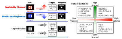
Figure 1. Experimental schematics of the task (left panel) and sample IAPS pictures selected in this study (right panel). Participants heard one of three conditioned auditory tones, each of which predicted upcoming picture to be a positive ('Predictable pleasant'), negative ('Predictable Unpleasant'), or either of those at 50% probability ('Unpredictable'). Pitch of tones indicated which condition that trial would be. A low tone, an intermediate tone, or a high tone corresponded with positive, unpredictable, or negative conditions (assignment for the high and low tones were counterbalanced across participants). After a 4000 msec inter-stimulus-interval (ISI), including 250msec of the tone, a picture was displayed for 4000 msec followed by a valence rating task after an image offset. During the ISI, participants were requested to imagine what type/kind of picture might be displayed. At the rating period, participants were required to rate emotional valence of the perceived picture at a 4 Likert-scale, ranged the most negative, more-or-less negative, more-or-less positive, to the most positive. The right panel shows sample pictures displayed in this study, mapped onto quadrants of valence and arousal axial model.
Download figure:
Standard image High-resolution imageDuring the 4000 msec blank period, participants were asked to imagine what kind of image would be displayed. After the delay, an emotion-triggering picture was displayed at the center of the screen for 4000 msec (for the details of the selected pictures, see the Stimuli section below). Following the picture display, a red fixation cross appeared at the center of the screen for 1000 msec. During this response period, participants were asked to rate their subjective feeling of valence by answering the question 'how were you moved by seeing that picture' on a 4-point Likert scale: 'strongly pleasant', 'pleasant', 'unpleasant' and 'strongly unpleasant'. They reported their response by pressing either the corresponding keyboard button with the thumb, index finger, middle finger, or ring finger (for EEG) or the response button (for fMRI). Before the main task, participants underwent a brief practice session for all three conditions with a picture set independent of that used for the main task.
2.3. Stimuli
As a predictive cue, one of three different auditory tones (500, 1000, or 1500 Hz) was played for 250 msec via a pair of headphones worn comfortably. Before the experiment, during the practice session, the volumes of the tones were checked with the participants and adjusted to comfortable levels. The 500 Hz (the low-frequency tone) or 1500 Hz (the high-frequency tone) stimuli could predict either a pleasant or unpleasant picture, and the 1000 Hz (the intermediate tone) stimulus was used as the unpredictive cue. The assignment of high and low-frequency tones was counterbalanced across participants. The intermediate tone was fixed for the unpredictive condition across all participants.
Novel images were carefully selected from 1182 pictures from the International Affective Picture System [IAPS; 29] with the following criteria. Pictures that might cause an excessively negative affect, such as corpses or the like, or that may be counter to our local ethics were discarded. In addition, the following pictures were disregarded: pictures consisting of multiple objects that could each be the object of focus of the participant; pictures with an intermediate valence that may not evoke an adequate intensity of either positive or negative valence such as plain scenery or objects (valence ratings between 4–6, see supplementary figure 1); and pictures containing text, symbols or items that may have cultural discrepancies (i.e. guns). The resulting 320 pictures were divided into two sets of 160 pictures (one for the tests for each of the two MRI sessions with 80 trials each and the other 160 pictures for the tests for the EEG session) randomly while controlling for average ratings (as reported in the IAPS dataset) of valence and arousal. Each set of 160 pictures was counterbalanced across participants. For each set of 160 pictures, half were pleasant, and the other half were unpleasant. Each picture appeared at least once for the two predictive cue conditions ('predictive pleasant' or 'unpleasant'). Half of the 160 pictures (both pleasant and unpleasant) were displayed twice for the unpredictive cue condition ('intermediate tone'). In the selected pictures, the brightness and spatial frequency (high or low; split at 140 Hz) of the visual features were adjusted such that they were not significantly different among different sets. In addition, the contents of each picture had been visually determined (human, animal, scenery, or others), and the categorical information was also equally distributed across the sets. See supplementary figure 1 for the details of valence and arousal ratings used in this study. All IAPS pictures were novel to the participants.
A Dell 24-inch LCD monitor was used to display pictures at a 1920 × 1080 pixel resolution. A chin rest placed 56 cm away from the monitor was used to stabilize the distance between the monitor and the eye for the participants. The sizes of the pictures varied. Some were oriented in landscape, and others were in portrait; however, the original pictures were displayed to fit the monitor. All auditory and visual stimuli were delivered by Presentation software version 17.2 (NeuroBehavioral Systems, San Francisco, USA).
As noted above, the trials consisted of fMRI and EEG sessions. All behavioral tasks remained the same; however, a total of 120 trials (including 40 repeated-pictures) were conducted for each of the fMRI sessions, and 240 trials (including 80 repeated-pictures) were conducted for the EEG sessions. On each visit, different sets of pictures were used to maintain the novelty of the pictures. For the EEG sessions, each cueing condition was presented for 80 trials, resulting in a total of 240 trials for the experiment. Regardless of cueing type, the participants judged 120 pleasant and 120 unpleasant pictures.
2.4. Subjective rating procedures
At the completion of the main task, the participants reported their subjective feelings by rating the pictures on a 0–100 visual analog scale for all conditions. Each question was displayed at the center of the screen, and a VAS was displayed underneath. Participants answered each question on the computer monitor by moving a pointer to the left (0) or the right (100) on the scale with the left or right arrow keys on the keyboard. The participants were instructed as follows: 'The following questions concern the evaluation of your feelings during the experiment. Once a question appears on the screen, please answer the degree of feeling experienced when you heard each tone on a scale between 0–100'. For each condition, participants rated the degree of 'valence' (unpleasant to pleasant; 'Kai' in Japanese), 'arousal' (low to high arousal; 'Kassei' in Japanese), and 'expectation' (low to high expectation; 'Kitai-kan' in Japanese), as well as 'Waku-Waku' ('a sense of exhilaration' or 'anticipatory excitement' in Japanese). For example, the sentence below appeared in the middle of the screen for the 'predictive pleasant' condition: 'Please rate the degree of "pleasure" (wellness of the feeling) when you heard the low-frequency tone.' A similar sentence was used for "arousal" (degree of liveliness), but for "expectation", the word was presented with no added explanation.
Here, we selected the term 'expectation' rather than a specific word such as 'prediction' or 'time'. This was because 1) we assumed that a predictive sense would be hard to report consciously and accurately; 2) we determined that 'time' (how soon they felt/expected) was inappropriate to ask, as the timing of the upcoming picture presentation was fixed to 4 sec. Furthermore, the definition of 'Waku-Waku' might depend on how the participant would conceptualize it. For the sense of anticipatory excitement, the term 'expectation' (Kitai-kan in Japanese) is supposed to reflect anticipation. However, it should be noted that one might not be able to adequately separate and ignore his or her own emotions that are covertly attached to the expectation when rating the expectation. The feeling of expectation might unconsciously induce emotional valence. We discuss the interpretation of these results with the derived correlations in results section 3.1 and the Discussion section; however, our choice of statistical procedure—a mixed linear model—would account for such putatively correlated inputs (see below for details).
As described above, each participant rated the pictures a total of three times for each of the experimental sessions (once for the EEG and twice for the fMRI experiments). All ratings were recorded for the analysis. Notably, the creation of a model with data from only 28 participants from one EEG experiment (one data point per condition) did not meet our statistical criteria for constructing a psychological model. We decided to include the data from all three sessions to ensure that all three axes achieved the desired level of significance.
2.5. Statistical analysis
The primary aim was to construct a formula with the anticipation of excitement ('Waku-Waku') as the dependent variable and three independent variable axes, namely, valence, arousal, and expectation. We first constructed a simple linear equation with the corresponding coefficients for each axis with no intercept. It should be noted that our primary aim was to obtain a starting point of reference to quantify the feeling of anticipatory excitement, 'Waku-Waku'. A mixed linear model was applied to obtain the weights for each axis (valence, arousal, and expectation) based on the subjective ratings for the anticipation of excitement with the 'Mixed Model' function in IBM SPSS version 22. The mixed linear model analysis is similar to a regression, but it can handle complicated situations similar to those in our case, where each subject participated in tests across multiple occasions (repeated design) and in different orders or with different picture sets (between-subject variability). Compared to the general linear model (GLM) that assumes independence across the data, the mixed linear model has an advantage in handling putatively correlated and unbalanced data. Notably, some degrees of correlations and random effects among the subjective ratings across the axes were assumed; a typical GLM approach might not be suitable in this case. The resultant psychological model, therefore, takes the putatively correlated effects into account. The assignment of counterbalanced tones, picture sets, the examined domains of the measurements (two MRI measurements and one EEG measurement), and the order in which the MRI or EEG measurement experiments were performed were included as covariates of no interest. In the mixed model function, repeated covariance type was set to 'scaled identity', and the maximum likelihood method was used to estimate the linear mixed model with 100 iterations. Estimates of the fixed effects were standardized and taken as coefficients for each independent variable.
As described above, the inclusion of at least valence and arousal from the original circumplex model was expected to be fundamental to the model. To validate the observed coefficients, the likelihood ratio test (χ2 statistic) was evaluated for each axis. All axes met the significance level (p <.05) as reported in section 3.1. The arousal axis did not meet the criteria when including only one of three sessions. That was one of the reasons to include the behavioral results from the MRI sessions, which otherwise could have been part of an independent study.
2.6. EEG procedures
2.6.1. Recording procedures.
During the task mentioned above, the participants' EEG data were recorded with a 64-channel BioSemi Active Two system at a sampling rate of 2000 Hz. The channels were placed according to the International 10–20 system layout. In addition, conventional vertical and horizontal electrooculograms were collected: approximately 3–4 cm below and above the center of the left eyeball for the vertical electrooculogram and approximately 1 cm to the side of the external canthi on each eye for the horizontal electrooculograms. An online reference channel was placed on the tip of the nose.
2.6.2. Analytical procedures.
Recorded EEG data were analyzed offline with the EEGLAB toolbox [30] running on MATLAB 2015 a (Mathworks, Inc), which was partly combined with custom-made functions. Continuous data were first DC-offset corrected, low-pass filtered with a two-way least-squares FIR filter at 40 Hz, resampled to 512 Hz, and epoched from 500 msec before cue onset to 8200 msec after cue onset (4200 msec after image onset). The epoched data were then rereferenced, and each channel was normalized to the baseline period (the 500 msec before cue onset). Any trials with excessive artifacts in the channels were rejected by the automatic artifact rejection model implemented in EEGLAB with an absolute amplitude threshold of more than 100 μV and probability over five standard deviations. Each iteration of artifact detection was performed with a maximum of 5% of the total trials to be rejected per iteration. In addition to the basic artifact rejection, we corrected artifacts derived from eye movements using conventional recursive least-squares regression (CRLS) implemented in EEGLAB [31] by referring to the vertical and horizontal EOG reference channels with a 3rd order adaptive filter with a forgetting factor (lambda, 'λ') of.9999 and.01 sigma ('σ').
The resulting corrected data underwent an initial independent component decomposition (also known as independent component analysis (ICA)) [30] to capture any artifactual activity that still survived our initial rejection criteria. Specifically, the logistic infomax ICA algorithm [32]—an unsupervised learning algorithm and a higher-order generalization of well-known principal component analysis that can separate statistically and temporary independent components in the signals—was used. It was followed by another run of automatic artifact rejection, now on the independent components (ICs), to remove artifactual components with the same criteria used for the channel-based rejection mentioned above. After the IC-based rejections, the artifact-free data underwent a second and final IC decomposition to extract independent neural activity, resulting in 64 putatively clean ICs per participant. Finally, fine-grained dipole analysis was performed using the 'dipfit' function in EEGLAB for each IC assuming one dipole in the brain. Supplementary figure 2 depicts the estimated dipole positions for each IC.
2.6.3. Rejection criteria.
Artifacts were rejected from the analysis according to the following criteria: any ICs with residual variances greater than 50% (equivalent to the proportion of outliers at p <.005, one-tailed; z-score >2.58); estimated dipole positions outside of the brain; or any ICs with an inverse weight only on one EEG channel of more than five standard deviations. This process retained an average of 33.89 ICs (range 26–43 ICs) per participant. A total of 949 ICs were retained for subsequent analyses.
2.6.4. Clustering independent components.
To quantitatively determine the number of IC clusters to be extracted, we employed a Gaussian mixture model (GMM) to cluster the ICs based on their scalp topography, and we iterated the GMM across the range of potential number of clusters (1 to 60). The number of clusters to extract was determined by Bayesian Information Criteria (BIC) due to its consistency over the Akaike Information Criteria [33, 34]. Because of the nature of ICA, the polarity of the IC scalp map is arbitrary. Therefore, the polarities of all retained ICs were aligned. The polarity of each IC weight was inverted, if necessary, such that all components correlated positively to each other. All the aligned data were then Z-score normalized across channels for each IC prior to the GMM analysis.
We iteratively clustered the 949 ICs with their inverse weights from the 64 channels by a GMM that maximizes likelihoods using the iterative expectation-maximization (EM) algorithm with the following rules. Covariance type was restricted to be diagonal; shared covariance was allowed, with an addition of a regularization value of 0.05. The maximum number of allowed EM iterations within each fit was set to 1000. We repeated the procedures for 1–60 clusters (we did not perform more than 60, as the decision could be drawn straightforwardly from this number). The lowest BIC value determined the best GMM with the corresponding number of clusters to extract. Finally, the centroids of the inverse weights for each cluster were computed, and then each IC was clustered based on the selected model for subsequent statistical analyses.
2.6.5. Spectrogram computation.
The preprocessed data were re-epoched from–500 to 4200 msec around the image onset for valence (seeing positive vs. negative pictures) and arousal (seeing high vs. low arousal pictures), and baseline correction was applied between–500 and 0 msec. Likewise, data were re-epoched from–500 to 4200 msec around the cue-onset for expectation (expecting a positive picture vs. unpredictive), and baseline correction was performed as before. It should be noted that both sets of epoched data shared the same ICs, as this epoch separation was performed after the final ICA so that we could equally compare the results before and after the image onset.
For all retained ICs, the spectrogram was computed between 0–4000 msec from the onset of the image for 'valence' and 'arousal,' and between 0–4000 msec after the onset of the cue for 'expectation.' For the sake of practicality and given its speed of computation in real-time, we applied fast Fourier transformation (FFT) on each set of segmented data with a Hamming window and zero padding to assess the frequency power density in different frequency bands. The resulting spectral power was then averaged for the θ (4–8 Hz), α (8–12 Hz), and β (12–20 Hz) frequency bands. One of the purposes of this study was to elucidate the neural correlates that would be efficiently applicable for academia-industry collaboration under the assumption that a wearable and dry-electrode EEG headset might be used in various environmental situations. Compared to active and wet EEG electrodes with low electrode impedances, dry electrode headsets are known to be susceptible to low signal-to-noise ratios [35], particularly at slow and fast frequency bands, which cover event-related potentials. Moreover, higher electrode impedances may also result from sweating, which strikingly diminishes data quality depending on the recording environment, especially in hot and humid environments [36]. Therefore, we focused only on those frequency bands that were likely to be reliable, with potential easy-to-use applications in mind.
Finally, we examined whether the spectral power of each IC could dissociate the valence, arousal, and expectation processes. The Wilcoxon signed-rank test was applied for each IC cluster (due to the nonnormal distribution of spectral power for most cases). This test was used to determine whether the frequency range of the IC could significantly differentiate the 'pleasant and unpleasant', 'high arousal and low arousal', and 'predictive pleasant and unpredictive' conditions for the expectation axis. The α-level was false discovery rate (FDR)-corrected, controlling for multiple comparisons across frequencies.
2.6.6. Evaluation of the proposed BEI model.
Among the three cueing conditions, our hypothetical choice for the third axis was set to only one of the paired comparisons as the expectation axis. As one may speculate, an alternative comparison could be proposed, but it requires validation. Additional analyses were performed on 'predictive pleasant vs. predictive unpleasant' and 'both predictive trials (predictive pleasant and predictive unpleasant) vs. unpredictive'. The former comparison assessed feasibility against the valence axis because of sharing a similar comparison before and after the image onset. This comparison might share some neural properties on its emotional values even before the image was seen. The latter contrast was examined as a counterpart for the expectation axis, provided we can assume expectancy regardless of emotional value as the third axis. The choice of the 'predictive pleasant vs. unpredictive' comparison as the expectation axis was based on the way we asked participants to rate 'expectation.' The term might reflect not only the predictability of an event ('how likely to expect') but also a positively biased degree of the mental imagery associated with the future ('how much to expect'). Because the probability of seeing a pleasant/unpleasant picture was radically fixed at 100% for the predictive cues, collecting subjective feedback for the likelihood (or predictability) might be redundant in this experimental design. Therefore, it was assumed that any neural features corresponding to only 'prediction' might fail to reflect 'expectation', which might be biased to positive anticipation.
We found the corresponding EEG features for each axis of interest. As a means to validate the BEI model based on the spectral power from the EEG data, the proposed model was evaluated by estimating the scores of each axis and then applied to formula (4) (see section 3.3 below). First, the spectral power of the selected frequency band of the selected ICs for all conditions was converted into a normalized score (0–100) for each IC. The normal cumulative distribution function was used to match spectral power (in units of decibels) to the VAS-scaled scores for Waku-Waku. For each axis, the obtained mean scores were then normalized across the three anticipatory conditions ('predictive pleasant', 'predictive unpleasant', and 'unpredictive') in which the participants rated Waku-Waku. It should be noted that the neural markers for valence and arousal axes were established based on the EEG data after image onset. Nevertheless, we intuitively applied these neural markers during the anticipatory period so that quantification of Waku-Waku could be achieved based on the same EEG data as that for the expectation axis. Finally, Waku-Waku was estimated by substituting the converted scores (0–100) into formula (4). Similarly, as a supplement to what the proposed BEI model could estimate, the transition of Waku-Waku was also quantified with the data obtained after the image onset period. As a comparison counterpart to the 'expectation' axis, each conditional value was estimated by the 'prediction' axis, as mentioned above.
3. Results
3.1. Psychological model of 'Waku-Waku'
See figure 2 for a summary of the subjective ratings for each cueing condition ('predictive pleasant,' 'unpredictive,' and 'predictive unpleasant'). Based on the ratings for valence, arousal, expectation, and Waku-Waku, the linear models with fixed weights were tested with valence and arousal as independent variables for a conventional two-dimensional model and with valence, arousal, and expectation as independent variables for a three-dimensional model. For both models, Waku-Waku was the dependent variable.
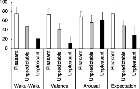
Figure 2.: Grand-averaged subjective ratings of anticipation of excitement ('Waku-Waku' in Japanese), valence, arousal, and expectation on a 0–100 scale for each cued condition: namely, predictive pleasant ('Pleasant'), unpredictive of either pleasant or unpleasant ('Unpredictable'), and predictive unpleasant ('Unpleasant'). These grand-averages were comprised of all three sessions per participant. Error bars represent 1 SD. As was expected, Waku-Waku was the highest for the predictively pleasant condition, followed by unpredictable and predictive unpleasant conditions. Ratings for valence were more or less similar to the anticipation but not necessarily the same. Arousal was rated equally across conditions. Expectation (see the main text for definitional differences between Waku-Waku and expectation) was similar to that of anticipation of excitement. A mixed linear model was performed on these subjective rating scores to model the anticipation of excitement. The resulting formula is reported in the main text.
Download figure:
Standard image High-resolution imageWith the 2-axis model, the result of the mixed linear model analysis (see Method section 2.5) revealed that 'Waku-Waku ("W")' was modeled with the estimates of the fixed effects of valence and arousal as follows (adjusted R2 =.90):

The 95% confidence intervals for valence and arousal were.66–.80 and.24–.35, respectively. Similarly, the mixed linear model for the three-axis model with the addition of the expectation fixed effect is depicted as follows (adjusted R2 =.93).
The 95% confidence intervals for valence, arousal, and expectation were.27–.46,.04–.16, and.46–.64, respectively. As expected, the three-dimensional model outperformed the two-dimensional model in terms of the accuracy by 3% of the variance. Notably, the added third axis of expectation was significant and highly loaded. When including only one of the experimental sessions, the coefficient for the arousal axis did not meet our criteria (at p <.05), but that of the valence and expectation axes did. For completeness, here are the fitted formulas for each session: [MRI1: W =.53*V +.04*A +.45*E; MRI2: W =.30*V +.12*A +.52*E; EEG: W =.29*V +.16*A +.61*E], where W, V, A, and E correspond to Waku-Waku, valence, arousal, and expectation, respectively. The values of the Akaike Information Criteria (AIC), an index that assesses the goodness-of-fit of each model, computed for each session (MRI1, MRI2, and EEG) with the three-axis models were 670, 686, and 669, respectively. This result implies that the formula for the EEG session might have been the best compared to those for the MRI sessions. However, the differences in the values among the three sessions were and negligible, indicating that the AIC values validate the comparability of the scores for all three sessions.
In addition, direct pairwise correlations were examined between Waku-Waku and each of the three axes. The resulting correlation coefficients (r2-values; p-values in parentheses) for valence, arousal, and expectation were.59 (p <.001),.04 (p <.005), and.66 (p <.001), respectively. These direct correlations roughly reflect the weight balance of the coefficients derived in formula (2). The correlations among the three axes were also examined. The resulting correlation coefficients for the valence and arousal, valence and expectation, and arousal and expectation pairs were.00 (.37),.55 (<.001), and.05 (<.001), respectively. Please note that the mixed model should have taken care of these correlations as well as the other unbalances or random effects from the samples. Supplementary figure 2 shows the scatterplots of Waku-Waku ratings as a function of the different axial counterpart.
3.2. Spectral EEG markers
From the GMM analysis on the inverse weights of the 949 ICs, a comparison of the BIC values for 1–60 clusters suggested that 15 clusters should be extracted. Figure 3 shows the BIC values across all examined numbers of clusters to be extracted (left panel) and the topographical IC maps for each common IC cluster (right panel; supplementary figure 3 also depicts the centroid coordinates of the dipole location for each cluster). Notably, these clusters of ICs are irrespective of the order of the identified ICs from the final ICA procedure. These clusters represent the shared ICs across subjects based on the topographical maps (inverse weights) of all ICs.
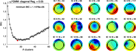
Figure 3. Bayesian information criteria (BIC) values of the gaussian mixture model (GMM) for each number of clusters (left panel) and 15 scalp topography of independent component (IC) clusters determined by the GMM (right panel). The number of clusters to extract was determined on BIC values. As it turned out, a model with 15 clusters (a red dot) was determined from 28 participants with 64 ICs per participant. 'N' corresponds to the number of ICs grouped in the cluster. For more details, see supplementary materials. Note, cluster number is not important here.
Download figure:
Standard image High-resolution imageSpectral power was examined for each IC cluster (see figure 4 for a summary of significant and marginally significant ICs; supplementary table 1 contains the statistical results of all IC clusters for completeness). For the valence (figure 4(a)), arousal (figure 4(b)), and expectation (figure 4(c)) axes, 5, 2, and 2 IC clusters emerged as significant, respectively. Emotional valence was represented by several EEG features that dissociated the pleasant and unpleasant conditions after picture onset, such as the θ-band of IC clusters 1, 5, and 7, the α-band of IC clusters 5 and 6, and the β-band of IC clusters 7 and 14. Of these, IC cluster 5 was shared by all sampled participants. Arousal was instead quantified by two IC clusters that differentiated the high- and low-arousal conditions after picture onset: the α-band of IC cluster 7 and the β-band of IC cluster 11. Of these, the α-band of IC cluster 7 was more reliable, shared by a greater percentage (86%) of participants. As expected, the θ-band of IC cluster 10 significantly dissociated the predictive pleasant and unpredictive conditions during the precue interval, and it was slightly more reliable than IC cluster 15, which also dissociated the above conditions.
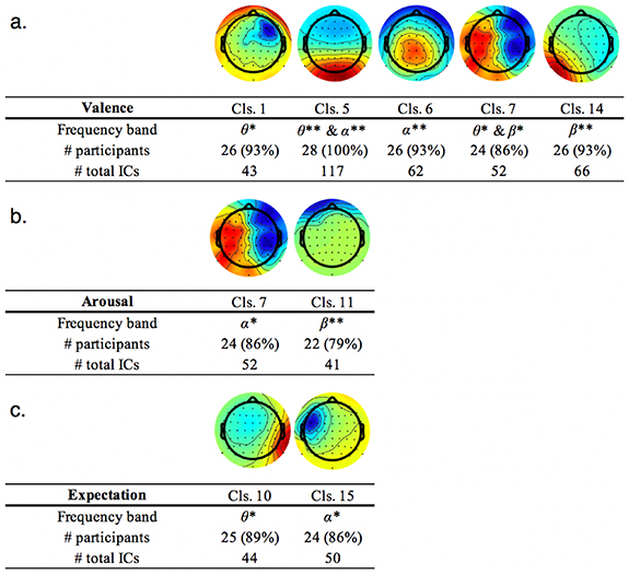
Figure 4. Scalp topographies of independent component clusters and their frequency ranges found to be significant for a) valence axis ('seeing positive picture' v.s. 'seeing negative picture'); b) arousal axis ('seeing high arousal picture' v.s. 'seeing low arousal picture'); and c) expectation ('Predictive pleasant' v.s. 'unpredictable, at 50–50 chance to see positive picture'). The number of participants who held an IC grouped into each cluster ('Cls.') and its percentage of participants relative to the sample size (n= 28) are listed as well as a total number of ICs belong to each cluster. Color intensities of either red or blue indicate a strong weight in the region. For our purposes, their red/blue color representation (either positive or negative) is not relevant as our focus of the analysis was solely on spectral power without consideration of the direction of the current. The color spectrum of red to blue may be flipped to represent the same IC. **Statistically significant at p <.05 FDR corrected; *Statistically significant at p <.05 uncorrected. For the full details of the statistics for all clusters, please refer to the supplementary table.
Download figure:
Standard image High-resolution imageSupplementary table 4 shows the results for all ICs, including marginally significant ICs, as well as additional supplementary comparisons focusing on 'predictive pleasant vs. predictive unpleasant' and 'both predictive conditions vs. unpredictive'. Some IC clusters were shared by all participants (100%), but some were not (i.e. valence cluster 11 for 79% of the participants). Across all comparisons, some IC clusters were shared on different axes, such as cluster 7 for valence and arousal at different frequency bands. No single IC cluster (and frequency band) survived the correction across all three axes.
3.3. 3-D linear BEI model
Given the three-dimensional psychological model (2) and corresponding neural correlates selected for each axis, we first propose a 'conceptual' BEI model to estimate Waku-Waku ('We') below. Assuming that formula (2) is valid and that the corresponding EEG features could estimate each axis value (ranging between 0–100), the psychological axes in formula (2) consist of subjective ratings that may be replaced with corresponding EEG features.

where EEGValence, EEGArousal, and EEGExpectation correspond to the normalized (0–100) spectral power of the ICs for the valence, arousal, and expectation axes, respectively. Here, a conversion of EEG spectral power from its standard unit (dB) to a normalized unit (0–100) is necessary because the unit acquired for the psychological model ranged between 0–100, while the spectral density of EEG signals does not span this range.
Given the statistical results, we selected the most robust and reliable IC candidates that survived our criteria because multiple EEG features were identified. The selection criteria were a combination of the highest Z-score and the highest proportion of participants who were covered by the selected IC cluster. The final selected formula for the estimated Waku-Waku (We) is expressed as
where IC5, IC7, and IC10 correspond to the IC clusters reported in figure 3, figure 4 and supplementary table 1; the θ and α in parentheses correspond to the frequency ranges of interest for each IC. It should be noted that as described in the above section, each EEG feature assumes that the values are normalized (0–100) within its power distribution. An example workflow using formula (4) is depicted in figure 5.

Figure 5. A conceptual workflow of quantification of 'Waku-Waku (anticipatory excitement, "W")'. In the linear equation, W is quantified by a combination of valence ('Val.), arousal ('Aro.') and expectation ('Exp.').
Download figure:
Standard image High-resolution imageIn figure 5, we propose an example BEI workflow. First, the raw EEG data from an epoch of 4000 msec is imported. The imported data are first preprocessed (including 4–20 Hz filtering and data mining) for subsequent quantification of the valence, arousal, and expectation axes. The filtered data are then sphered to extract the independence across channels. The IC weights of interest are extracted from the sphered data, and the spectral power density for each target frequency band (θ of IC5 for valence, α of IC7 for arousal, and θ of IC10 for expectation, as determined in section 3.2; see also figures 3 and 4) is obtained. The obtained spectral power is then scaled to a normalized unit (0–100) based on the prior distribution of the spectral power of each IC candidate. Here, the prior distribution of each EEG feature may be assessed from the entire collected data for offline analysis. Alternatively, for a real-time workflow, the prior distribution may be constructed by collecting a certain duration of data as a calibration stage prior to running the above workflow. Finally, the coefficients for each axis are combined with the normalized EEG features as in formula (4). With the rescaled EEG features, the final values for valence ('Val.'), arousal ('Aro.') and expectation ('Exp.') are replaced by the values obtained from the EEG data as in formula (4).
3.4. Validation of the neural markers and the 3-D linear model
Although we proposed a hypothesis-driven BEI model to quantify Waku-Waku with three putatively separable axes with corresponding neural markers, the model still requires validation with existing data samples. Although robust interpretation may be limited, we performed three additional analyses: 1) the spectral power of the ICs were compared for the contrast between 'predictive pleasant' and 'predictive unpleasant' to compare against the valence and expectation axes; 2) the spectral power of the ICs were compared for 'predictive' and 'unpredictive' to derive a potential predictive axis and compare it against the expectation axis; and 3) the estimated Waku-Waku was computed and compared against the subjective ratings for each condition.
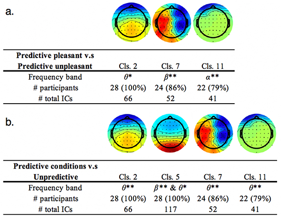
First, we compared EEGs for the directly contrasting conditions in which Waku-Waku was rated the highest (predictive pleasant) and the lowest (predictive unpleasant). This contrast is unsuitable as a neural response for anticipation because it conceptually subtracts out the predictive component. However, this contrast might provide informative insight on a comparison with the valence ('seeing pleasant' vs. 'seeing unpleasant') or expectation ('predictive pleasant' vs. 'unpredictive') axis. Figure 6 below shows the results of the additional analyses: the θ-band of IC2, β-band of IC7, and θ and α-band of IC11 were significant (see supplementary table for the details).
Table 1. Estimated scores for each axis and Waku-Waku for the cue-onset (anticipatory) period and the image-onset period. 'We' represents the final estimated Waku-Waku score by the proposed model with an axis of expectation ('predictive pleasant' v.s. 'unpredictive' conditions) as the third axis. 'Wp' represents Waku-Waku scores estimated by a counterpart model with the third axis replaced by a contrast of prediction ('two predictive conditions' v.s. 'unpredictive' conditions). The main point of comparison would be the result for the cue-onset, where Waku-Waku and all the subjective ratings were collected. Estimations of Waku-Waku for the image-onset are performed for speculation purposes only. The Waku-Waku scores of the two variant models indicate that our proposed model with the expectation axis outperforms that with the prediction.
| Valence | Arousal | Expectation | Prediction | We | Wp | ||
|---|---|---|---|---|---|---|---|
| Cue-onset | Predictive pleasant | 54 | 88 | 87 | 41 | 76 | 52 |
| Unpredictable | 83 | 26 | 22 | 19 | 46 | 44 | |
| Predictive unpleasant | 15 | 31 | 36 | 86 | 28 | 54 | |
| Image-onset | Pleasant | 89 | 61 | 23 | 86 | 53 | 85 |
| Unpleasant | 13 | 41 | 80 | 14 | 51 | 17 | |
| High arousal | 60 | 88 | 81 | 29 | 75 | 47 | |
| Low arousal | 35 | 11 | 16 | 72 | 23 | 52 |
Figure 6. Scalp topographies of significant independent component clusters and their frequency ranges. (a) Conditions in which subjective ratings were the highest and lowest were compared, 'predictive pleasant' and 'predictive unpleasant', respectively. (b) Conditions of the maximum expectancy regardless of emotional valence (100%) and lowest (50%) expectancy were compared, 'two predictive conditions combined' and 'unpredictive', respectively. **Statistically significant at p <.05 FDR corrected; *Statistically significant at p <.05 uncorrected.
Download figure:
Standard image High-resolution image
To further supplement the inspection, another comparison was performed on the two predictive conditions combined vs. the unpredictive conditions. In principle, this contrast supposedly reflects the anticipation of emotionally salient images regardless of their emotional value (either pleasant or unpleasant) with respect to the emotionally vague condition. Therefore, this contrast could have theoretically replaced the expectation axis. The θ-band of IC2, β-band of IC5, θ-band of IC6, and θ-band of IC11 were found to be significant.
Finally, the proposed BEI model was applied to the existing data by estimating Waku-Waku values based on the given spectral power distributions across the conditions. It was assumed that Waku-Waku can be quantified with the three dimensions, provided the existence of at least one target EEG feature for all axes. However, 22 out of 28 participants held all of the corresponding ICs in our proposed model, and 24 out of 28 held all corresponding ICs with 'prediction (IC cluster 5)' as the third axis.
The table below summarizes the estimated score for each axis and the final Waku-Waku score for each condition. As was expected, using the statistically significant EEG features selected in formula (4), the scores for each axial contrast straightforwardly reflected each pair of contrasts (i.e. the valence scores for the pleasant images were estimated higher than those for the unpleasant images, etc). More importantly, the main candidate of this study, Waku-Waku, seemed to well quantify the subjective ratings for each condition, as shown in figure 2. Waku-Waku was rated the highest for the predictive pleasant, followed by the unpredictive and predictive unpleasant conditions. Given that our proposed model ('We') is valid, anticipating a highly pleasant and arousing picture might drive excitement the most, while anticipating a picture with unpleasant and less arousal drove it the least. It should be noted that only one value per condition is reported and without its mean or standard deviation because this estimation was performed from the average of all EEG features for each axis.
As a counterpart model for the third axis, an alternative model of Waku-Waku ('Wp') was examined by merely replacing the third axis with 'prediction' regardless of emotional valence (the 'unpredictive' vs. 'predictive pleasant combined with predictive unpleasant' contrast). As an EEG feature for this axis, the θ-band of IC cluster 5 was selected as a candidate. The estimated score did not follow the trend achieved by the proposed model. The estimated Waku-Waku scores for the 'predictive pleasant' and 'predictive unpleasant' conditions were higher than those for the 'unpredictive' condition; however, it seemed that the score for the 'predictive unpleasant' condition was the highest, in which Waku-Waku was supposedly the lowest instead.
4. Discussion
We proposed a prototypical BEI model to quantify the 'Waku-Waku' emotion toward upcoming visual images using neural markers based on the EEG and incorporating a three-dimensional psychological model.
4.1. 3D Psychological model.
First, a psychological task was given to participants to visually trigger their emotions. The participants were required to engage in anticipation of upcoming stimuli and to report their subjective feelings as they were anticipating one of three conditions (predictive pleasant, predictive unpleasant, and unpredictive) on four factors: 'Waku-Waku,' valence, arousal, and expectation. As was expected, the 3-D psychological model of 'Waku-Waku' including an axis for 'expectation', achieved an adequate fitting accuracy. As quantified by the adjusted R2 values, the fit of the 3-D model was better by 3% than that of the 2-D model. The improvement of the fit may be trivial to our aim, but the results indicate that the multiaxis model of emotion may be feasible to adapt.
Additionally, the 3-D model revealed a high loading on the third axis relative to that of the remaining two axes that the classical 2-D circumplex model of emotion would propose [1]. It assures that the subjective feeling of 'Waku-Waku' may be intimately linked to anticipation, followed by momentary emotions of pleasure and arousal. We also found that the two subjective ratings of valence and expectation moderately correlated with that of Waku-Waku, but they were not equal (the correlation coefficient (r2) was not very strong). These results suggest that the association between expectation alone or valence alone with Waku-Waku were not the same but both factors reflected a subset of Waku-Waku feelings to some extent. This result was plausible because 'Waku-Waku' is described as the state of one's heart being moved due to being pleased and expecting something pleasant. Therefore, both valence and expectation may be assumed to be highly loaded. Nevertheless, as was discussed earlier, Kansei—our instantaneous mental state of emotion—may be modeled by multifold human affects and cognition [6–8, 11]. Furthermore, the resultant variations in the coefficients for valence, arousal, and expectation suggest that the three aspects of psychological dimension differentially contribute to the feeling of Waku-Waku.
A psychological model should not be restricted by these proposed axes (valence, arousal, and expectation). In particular, the concept of the third axis in our case was a conceptualization of the time domain; however, any other dimensions associated with the human senses may be adapted. According to another 3-D emotional space model (pleasure, activation, and dominance, also known as the PAD model), dominance [37] could have been the third axis, and one could also build a nonlinear model as well. As discussed below, a sense of prediction that may putatively reflect a likelihood of expectation may also be a key factor because it is rooted in the concept of predictive coding. Furthermore, a psychological constructionist approach assumes emotion to be the interplay of the multiple brain networks that may require potentially more than three dimensions or other sophisticated methods [6]. Nevertheless, it is plausible to propose that the modeling our putatively complex nature of awareness would benefit from a multidimensional model.
4.2. Corresponding electrophysiological markers for the three axes
To determine the neural correlates for each axis of the BEI, the spectral power of the ICs of the EEG data were analyzed. The valence and arousal axes were quantified from the duration over which the participants visually observed the emotion-triggering picture. The expectation axis was determined from the delay period in which the participants anticipated the upcoming picture according to the played auditory cue, which was tied to valence type. A conventional spectral power analysis was performed for each IC, and dissociable neural markers were identified for each axis. This dissociation is one of the essential aspects of the validation of our model. Because the multidimensional model assumes the independence of the psychological axes and their corresponding neural markers, it was necessary to confirm that the EEG features selected for each axis were also dissociable. For example, a previous study suggested that multiple ICs could be loaded onto one axis and that one IC might also contribute to the other axes to some extent [38]. In addition, some studies support the view that the functions of a brain region are ubiquitous and not limited to unitary and discrete functions [6]. Therefore, we are not necessarily stringent with regard to this overlap; however, a complete overlap between any one pair of axes would be another story. If the same EEG features entirely correspond to a pair of axes, it may suggest that the pair would represent the same neurophysiological system. As a result, this would violate the assumption of the multidimensional model, making the addition of a new dimension meaningless. However, our results minimized the possibility of this dimension redundancy. There was no complete overlap across the three axes, supporting our proof of concept. The three-dimensional model could plausibly reflect putatively dissociable neural mechanisms. Below, we discuss the outcomes for each axis.
4.2.1. IC markers of valence.
For the valence axis, among several significant EEG features (θ-band of IC1, θ & α-bands of IC5, α-band of IC6, θ & β-bands of IC7 and β-band of IC14), the θ-band of IC cluster 5 was robustly significant. This component was also observed in all (100%) of the participants. Previous neuroimaging research suggests that a source in proximity to the orbitofrontal areas may be responsible for emotional valence [39]. A similar EEG study [38] related EEG features to subjective feelings at rest rather than those generated during a task based on the PAD model. By focusing only on the β-band power of the IC clusters, the authors found that IC clusters with sources localized in the posterior cingulate and right posterior temporal lobe were positively correlated with valence. In our study, the estimated dipole of clusters 6 and 7 was centered around the mid- to posterior- cingulate regions, in close proximity to that from their findings (see supplementary figure 2). Notably, the β-band of cluster 7 was also significant, validating the replicability of this neural source for emotional valence. However, in our case, because the number of participants who held this component was relatively small, we selected the alternative target with its significant frequency band in the θ-band instead. This IC could have been a reliable candidate for valence if the sampled population differed. The relatively slow oscillation of the θ-band might reflect the processing of visual information, which may be associated with remotely interconnected reward networks such as those in the midline orbitofrontal and anterior cingulate regions reported in fMRI studies [13].
4.2.2. IC markers for arousal.
For the arousal axis, neural activities evoked by seeing a picture with high arousal (i.e. a picture of fireworks or explosion, etc) were compared against those evoked by seeing a picture with low arousal (i.e. a picture of a calm scene of a house or a kitten, etc). Because of a slight difference in the reliability across participants, the α-band of IC cluster 7 was selected as the best target. Another prominent candidate was the β-band of IC11; this component might have been selected as an alternative. α-band oscillations elicited from the parietal regions typically reflect human arousal [22–24]. Our results suggest that α-band activities potentially located around the midline part of the brain (cingulate cortex) may reflect arousal. Although we carefully selected pictures based on their visuophysical properties, some physical features of the pictures, such as luminance or brightness, instead of their content might covertly trigger some EEG signals unrelated to the subjective feeling of arousal. Future studies may need to investigate this to rule out some potentially confounding factors.
4.2.3. IC markers for expectation
For the expectation axis, we contrasted the neural activities elicited when expecting a pleasant picture to those elicited when the valence of the expected picture was unknown. The θ-band of IC cluster 10, with its dipole centered at the right angular gyrus (in proximity to the inferior parietal lobule and lateral occipital complex regions), was significant. This region is known to be responsible for visuospatial attention [40] or maintenance of visual information in memory [41]. Another candidate was the α-band of cluster 15, with its localized source around the dorsolateral prefrontal cortex (DLPFC), typically nominated as a central source of executive functions [42, 43]. Accumulating research also suggests that this region plays a pivotal role in the integration of emotion and cognition [13]. Notably, studies of depression and emotional valence often refer to the hemispheric asymmetry of the α-band with its sources in this prefrontal region [44, 45], which is widely applied in BCI research aiming to treat depression [46, 47].
Again, it is possible that we might observe the same or similar neural markers for the expectation axis as for the valence axis because they differed only in whether the participant was mentally anticipating or actually seeing a picture on the monitor. One may speculate that the contrasts for the valence and the expectation axes might overlap. However, a similar approach with fMRI [48] indicated that lateral occipital regions were activated while seeing emotional pictures (after picture onset) rather than while expecting them (before picture onset). When expecting them, the anterior and posterior cingulate regions were responsible for the expectation of valent pictures compared to neutral targets. One may argue that methodological differences between EEG and fMRI are responsible for these observations, as EEG may be suitable for detecting electrical discharges while fMRI tracks cerebral blood flows as a result of neural activations. Another putative explanation may be that in our comparison, we did not have pictures with neutral valence. In our design, even for the unpredictive condition, the anticipated imagery and subjective ratings for this condition fluctuated between the two extremities of pleasant and unpleasant across participants (see supplementary figure 2); therefore, this unpredictive condition would not be the same as expecting a neutral image. Detailed investigations are necessary to further discuss the overlap between the location of dipoles and BOLD responses obtained from fMRI studies.
Nonetheless, previous fMRI research supports the concept of dissociable networks for emotional expectancy and emotion perception [48], corresponding to the expectation and valence axes, respectively. Regarding EEG studies on expectancy, several neural markers, such as late positive potentials, readiness potentials, or some other preparatory EEG markers, reportedly influence the expectancy of emotional items [49–51]. In our results, expectancy processes might recruit a combination of the executive network and the visuospatial network to anticipate by forming a mental imagery. Our findings on this axis may contribute to the field of expectancy. In reality, a sophisticated interplay of these higher cognitive functions may be associated with the expectation of emotional events. Notably, the selected neural marker for the expectation axis was also dissociable from those found to be significant for the valence axis. This neural level of dissociation indirectly assures that these two psychological dimensions would also be distinct even that the psychological ratings of the two would be correlated to some extent. It may also support the notion that the inclusion of the expectation axis may benefit from quantifying dissociable neural processes underlying the ubiquitous interplay of cognitive and affective functions [6].
4.3. Alternative comparisons and validation of the BEI model
In this study, the subjective ratings of Waku-Waku and the other axial factors were not collected for every trial. However, as an attempt to validate the neural markers found in the three axes, we directly contrasted the conditions in which Waku-Waku ratings were the highest ('Predictive pleasant') and lowest ('Predictive unpleasant'). Conceptually speaking, the valence axis and this contrast might have shared the same EEG features because both contrasts putatively compare emotionally pleasant and unpleasant images. The only difference between the two was whether participants were seeing an actual image on the screen or forming a mental image. We found that no EEG features overlapped between the two contrasts. This may imply that the neural mechanisms associated with expecting a future with uncertainty and those associated with exogenously confronting a reality at present may be dissociable. To reiterate, the inclusion of anticipation was fundamental to our model to estimate Waku-Waku. Therefore, it was presumed that the EEG features selected here would not represent the expectation axis because they would eliminate this valuable perspective of anticipatory neural function by contrasting the two predictive conditions.
Another potential contrast was made on 'the two predictive conditions combined' vs. the 'unpredictive' condition. Several neural signatures emerged on this axis, and they could become a counterpart for the third axis of expectation. The selected EEG feature for predictability successfully quantified the anticipatory conditions to some extent. However, the estimation of Waku-Waku with this axis (Wp) failed to follow the subjective ratings. See table that indicates that the predictive axis rated the highest ('86') when the cue was predictive unpleasant, whereas the estimated prediction value for the predictive pleasant condition was only 41. It might have been true that participants might 'predict' an occurrence of unwanted images; however, this contrast was not sufficient to represent the 'expectation' axis. Although the fit was not great for Waku-Waku, it does not necessarily mean that this axis of prediction could not be a part of a multiaxis model of emotion. It may be possible that the neural responses for the predictive unpleasant condition (somewhat associated with an emotion of worry) might be stronger than those for the predictive pleasant condition. If the experimental design of the way participants performed the task was more closely related to the prevalence, or entropy, of expectation regardless of emotional value, such a prediction or certainty axis with its selected components might have been a proper candidate for the third axis. Altogether, this axis was not suitable for our proposed model for Waku-Waku. Finally, it would be plausible to believe that the EEG feature we selected for the contrast between the 'predictive pleasant' and 'unpredictive' conditions was appropriate for our model.
5. Conclusion
We proposed a prototype BEI based on a multiaxis, three-dimensional model of emotion to quantify our anticipatory excitement using EEG. The fidelity of the BEI should be examined in future studies; however, provided a certain degree of accuracy backed by statistical results, our BEI may be able to quantify Kansei and be applicable at least for young adult Japanese (or Asian) individuals. In our group-level analysis, we found only a subset of IC and their corresponding frequency band for each axis; however, our result may not be conclusive due to putative cultural or age differences. Additionally, as our EEG-based BEI model was proposed only for visual stimuli, similar experiments or a generalization need to be tested with stimuli for other modalities, such as audition and touch.
Moreover, we found that the number of ICs shared by our participants was not perfect, especially because not all participants shared some of the key IC clusters selected for the arousal and expectation axes. This implies that the currently proposed BEI model may not be generalizable for all individuals, even within our collected samples. A close investigation and individual optimization for selecting ICs and their frequency ranges may be necessary to achieve full compatibility of the BEI. We applied the GMM method to determine the number of ICs to extract. While this method may be a quantitative means to determine the number of clusters, this approach tends to fluctuate with slightly different parameters. Alternatively, it may simplistically differ in a different ethical, cultural, or age population. Therefore, one should be careful when applying the results observed here to different groups. Based upon a fixed-effect model derived by determining a group-average model, we selected a fixed EEG feature across participants. Recent neuroscience studies instead propose that the individually optimized decoding of neural activities outperforms group-level approaches [52, 53], potentially associated with neuroarchitectures that differ across age [54, 55] or personality [56–58]. It is indeed plausible that individual optimizations of psychological, neural, or both models may provide accurate quantification of our feelings.
Our observations in this article may be limited in various aspects; however, this should constitute a reasonable basis to quantify our sense of Kansei. There are wide varieties of BCIs that exist in the field, and our approach of considering multiple axes combined with EEG markers may become a new tool for neuroscientific consultations. Such a tool may be applicable not only for stable pictures (i.e. art, pictures, advertisement posters, etc) but also for various other situations, such as motion pictures (i.e. movies, TV commercials). The application of BEIs may certainly require further evidence and theoretical support. With proper combination of hardware devices and software infrastructures, the BEIs may become useful tools for Kansei engineering in the near future.
Acknowledgments
Patents (PCT/JP2016/003712; JP2016116449A; US15/768,782; EP16855084.6A) have been submitted based on the part of described methods in this manuscript. Of those, a patent Japanese Patent 6590411 has been approved.
All authors discussed the manuscript. M.G.M., N.K., K.M., T.S., and S.Y. designed the behavioral paradigm. N.K. and K.M. prepared experimental materials and collected data. MGM, N.K., and R.M. performed the EEG analyses. M.G.M. and G.L. designed and built the brain computer interface. M.G.M., N.K., and G.L. wrote the manuscript. We highly appreciate Professor Hirokazu Yanagihara at Hiroshima University for his mathematical advice on this project.
This research was supported by JST COI Grant Number JPMJCE1311. G.L. was supported by the New Energy and Industrial Technology Development Organization (NEDO), by ImPACT of CSTI and by the Commissioned Research of NICT.
Supplementary data (2.4 MB PDF)