
Abstract
Objective. Understanding the neurophysiological signals underlying voluntary motor control and decoding them for prosthesis control are among the major challenges in applied neuroscience and bioengineering. Usually, information from the electrical activity of residual forearm muscles (i.e. the electromyogram, EMG) is used to control different functions of a prosthesis. Noteworthy, forearm EMG patterns at the onset of a contraction (transient phase) have shown to contain predictive information about upcoming grasps. However, decoding this information for the estimation of grasp force (GF) was so far overlooked. Approach. High density-EMG signals (192 channels) were recorded from twelve participants performing a pick-and-lift task. The final GF was estimated offline using linear regressors, with four subsets of channels and ten features obtained using three channels-features selection methods. Two different evaluation metrics (absolute error and R2), complemented with statistical analysis, were used to select the optimal configuration of the parameters. Different windows of data starting at the GF onset were compared to determine the time at which the GF can be ascertained from the EMG signals. Main results. The prediction accuracy improved by increasing the window length from the moment of the onset and kept improving until the steady state at which a plateau of performances was reached. With our methodology, estimations of the GF through 16 EMG channels reached an absolute error of 2.52% the maximum voluntary force using only transient information and 1.99% with the first 500 ms of data following the onset. Significance. The final GF estimation from transient EMG was comparable to the one obtained using steady state data, confirming our hypothesis that the transient phase contains information about the final GF. This result paves the way to fast online myoelectric controllers capable of decoding grasp strength from the very early portion of the EMG signal.
Export citation and abstract BibTeX RIS

Original content from this work may be used under the terms of the Creative Commons Attribution 3.0 licence. Any further distribution of this work must maintain attribution to the author(s) and the title of the work, journal citation and DOI.
1. Introduction
Understanding the neurophysiological signals underlying voluntary motor control and decoding them for controlling limb prostheses are among the major challenges in applied neuroscience and biomedical engineering. A case study of particular interest is represented by individuals with below-elbow amputation. Indeed, these people maintain part of the 18 extrinsic muscles that originally served the fingers and wrist and the electromyogram (EMG) recorded from these muscles can in theory be used to control a variety of grasps and movements in a multi-digit hand prosthesis.
Although significant efforts have been spent in decoding the user motor intent to seamessly control different motor functions of a hand prosthesis [1, 2] the estimation of the desired grasp force (GF) produced by the muscle from the EMG, has been investigated less extensively. As an example, the clinically adopted strategy in prosthetic hands consists in setting the GF proportional to the envelope of the recorded EMG signals [3], following an approach proposed by Bottomley [4] back in the sixties. However, it is well known that the relationship between the EMG and the output force produced by voluntary muscle contractions is not necessarily proportional [5, 6]: in fact, the force is modulated by the number of motor units (MU) recruited and their activation frequency [7, 8].
So far researchers have investigated this relationship using either intra-muscular [9–12] or surface EMG recordings [10–28]. Several estimation techniques, exploiting a wide range of methodologies, were proposed (table 1). In general, to provide this estimation, the EMG signals are decomposed into time segments using sliding windows and statistical features descriptive of the signal are calculated [29]. Then, the features are fed to a fitting algorithm (e.g. a classifier or a regressor) that provides an estimate of the force for each segment. By using several different algorithms, such as regressors [9, 11, 16, 17, 22, 24, 25] or artificial neural networks [9, 11–14, 21, 26, 27], these studies demonstrated notable estimation accuracies up to 0.95 R2 (coefficient of determination) or 4.21% absolute error (AE) from wrist, finger and trunk movements, and from a wide range of forces (e.g. from 0% to 100% of muscle activation [10, 11, 13, 15–17, 19, 22, 23, 25, 26], or up to 300 N of output force [9, 12, 14, 18, 24]). Notably, some of the methods developed for the estimation of the grip force from the EMG also allow for the simultaneous control of up to 6 degrees of freedom of a prosthesis [12, 15, 17, 20, 25, 27]. This is particularly interesting in clinical settings, where multi-articulated hand prostheses are now available, as these solutions also provide a smooth way to switch between motor functions of the prosthetic device (table 1).
Table 1. Literature about force estimation from EMG signals.
| Reference | Number of participant | Force range | Force patterns |
Muscles (number and type of electrodes) |
Algorithm | Error type | Accuracy |
|---|---|---|---|---|---|---|---|
| This study | 12 | 250 g to 1000 g | Pick and lift | Forearm ([4 8 16] 164s high density) | Regression | (500 ms after the onset) | |
| AE (%GFMVC) | 1.99 (1.04) | ||||||
| ~5% to 25% GFMVC | |||||||
| AE (N) | 0.64 (0.24) | ||||||
| R2 | 0.82 (0.16) | ||||||
| Liu et al [22] | 3 | 30% MVC flexion and extension | Profile | Forearm (128s high density) | Regression | AE (%MVC) | 4.21–10.20 |
| Potvin et al [23] | 8 | 0% to 100% MVC | Profile | Trunk (3s) | Nonlinear model | AE (%MVC) | 9.2 ± 2.6 |
| Hoozemans et al [24] | 8 | Dynamic force bursts up to 300 N | Dynamic force bursts | Forearm (6s) | Regression | AE (N) | 27–41 |
| Clancy et al [25] | 10 | 30% MVC | Profile | Forearm (16s) | Regression | RMS (%MVC) | 6.7–8.5 |
| Bøg et al [10] | 11 | 0% to 100% MVC | Profile | Forearm (1s and 1i) | Feature profile | R2 | >0.9 |
| Baldacchino et al [26] | 40 | 0% to 80% MVC | Profile | Forearm and upper arm (12s) | ANN | R2 | 0.91% ± 0.05% |
| RMS | 4.14% ± 0.92% | ||||||
| Nielsen et al 2011 [27] | 10 | Subjective low to medium | Movement | Forearm (7s) | ANN | R2 | 0.90 ± 0.02 |
| Kamavuako et al [9] | 10 | 0–50 N | Profile | Forearm (1i) | Regression and ANN | R2 | 0.89 ± 0.02 |
| Zhang et al 2018 [28] | 10 | 20, 40, 60% MVC | Profile | Forearm (8 × 16 s high density) | Regression | R2 (%MVC) | 0.78–0.93 (20–60 %MVC) |
| RMS (%MVC) | 15%–8% (20–60 %MVC) | ||||||
| Cao et al [13] | 10 | 100% MVC (<10% discarded) | Profile | Forearm (6s) combinations with 2–6 muscles | ANN | RMS ± Correlation coefficient | 1.165 ± 0.475 |
| SVM | 0.806 ± 0.254 | ||||||
| Regression | 3.369 ± 1.457 | ||||||
| Li et al [14] | 15 | 8 force levels 0–40 N | Level | Forearm (8s) | ANN | SD (N) | 3.58%–1.25% |
| Mirzakuchaki et al [15] | 10 | 0% to 80% MVC | Profile | Forearm and upper arm (12s) | Generalized regression neural network | R2 | 0.93% ± 0.05% |
| RMS | 0.057 ± 0.012 | ||||||
| Wang et al [16] | 6 | 0, 2, 4, 6, 8, 10 kg | Movement | Forearm (2s) | Regression | Average recognition rate | 92.57% ± 11.7% |
| Zhu et al [17] | 5 | ±30% MVC | Movement | Forearm (16s) | Regression | RMS (%MVC) | 6.0–16.3 |
| Gailey et al [18] | 8 | 6–30 N (sum of finger's) | Movement | Forearm (5s) | Random forest regression | RMS ± SE (%MVC) | 17 ± 2–26 ± 6 |
| Yang et al [19] | 6 | 10, 40, 70 and 100 %MVC | Level | Forearm (8s) | Genetic algorithm | RMS (%MVC) | 0.05 |
| Correlation Coefficient | 0.99 | ||||||
| Jiang et al [20] | 12 | Low to medium | Movement | Forearm (8s) | NMF | R2 | 0.90 ± 0.006 |
| Smidstrup et al [11] | 11 | 0%–100% MVC | Profiles | Flexor digitorum profundus (1s and 1i) | Regression | R2 | 0.95 ± 0.007 |
| Ameri et al [21] | 10 | Medium level | Movement | Forearm (8s) | ANN | R2 | 0.90 ± 0.005 |
| Kamavuako et al [12] | 10 | ±3 Nm and ±2 Nm | Profiles | Forearm (6i and 6) | ANN | R2 | 0.93 ± 0.03 |
aThe force requiring to follow a Profile (ramp, step, bell, etc), corresponding to a Movement (grasp, flexion, etc) or achieving a specific Level. bSuperficial (s) or intramuscular (i) electrodes. cThe accuracy is reported in terms of median (inter quartile range) or mean ± standard deviation.Some of the studies included several configurations, movement recognition or results with amputees. For brevity and comparison with the present study, only the best predictions on able-bodied participants are shown.
From an engineering perspective a voluntary muscle contraction may be divided in two phases, namely the transient and the steady state. The transient is associated to the bursts of myoelectric activity due to sudden muscular effort while executing a movement. It is related with the beginning of the recruitment of the MUs involved in the muscle contraction. The steady state corresponds to the part of the contraction when almost every MU involved in the movement is already recruited, that is, the myoelectric signal produced by a stable muscle contraction. The latter has very little temporal structure (it is mostly a random signal) due to the active modification of recruitment and firing patterns of the MUs needed to sustain the contraction [30]. On the contrary, the transient EMG was shown to possess a deterministic structure [29, 31], likely due to an orderly recruitment of the MUs. This indeed was demonstrated to be descriptive of the intended movement [31]. However, thus far, such temporal arrangement was poorly exploited for the estimation of the output force during a movement (table 1, [9–28]). Here we hypothesized that the informative content of the transient EMG in humans is likely due to the preplanned nature of grasping, in general, and of the final GF, in particular [32]. Thus, to estimate such a final GF, the information contained during the preliminary grasping phase could be sufficient. To the best of our knowledge only Calvert and Chapman attempted to decode the GF of the hand from the transient EMG, back in 1977 [33]. This pioneering study showed unsatisfactory results and concluded that, with the techniques of the time, it was not possible to obtain reliable estimates of the GF in the transient phase.
The objective of this work was to assess, using modern techniques, the viability of extracting relevant information from the transient phase of the EMG signal, in order to decode the target GF during a grasp. To this aim, we collected 192 monopolar channels of high density (HD) surface EMGs from the forearms of 12 able-bodied participants while producing highly repeatable GFs, i.e. performing pick and lift series of a test-object with different weights (250 g, 500 g, 750 g, 1 kg). Ten features were extracted from the HD-EMGs and the GFs decoded using three channels-features selection methods (fixed, partially fixed and automatic) were assessed offline and compared. Our results show that is possible to estimate the GFs using down to 16 channels, with an AE of 1.99% of the maximum voluntary force using information from the first 500 ms of data following the GF onset. These results pave the way to online myoelectric controllers capable not only of decoding the intended grasp type but to do so from the very early portion of the EMG signal.
2. Materials and methods
2.1. Experimental protocol
Twelve able-bodied participants (aged 27.6 ± 2.96 years, seven males, all right-handed) without any history of neuromuscular disorders participated to this study. Written informed consent in accordance with the Declaration of Helsinki was obtained before conducting the experiments from each participant. This study was approved by the local ethical committee of the Scuola Superiore Sant'Anna, Pisa, Italy (request no. 02/2017). The methods were carried out in accordance with the approved guidelines. The experimental setup consisted of a test-object instrumented with force sensors, an object stand with embedded load cells, a chair with an instrumented armrest, an HD-EMG recording system and a PC (figure 1(a)).

Figure 1. Experimental setup. (a) Lateral view of the participant, with his right hand resting on the starting position sensor (in purple) and with the test-object on top of the stand (green) and monitor in line of sight. (b) Test-object consisting of a handle (red) and a box (blue). Dimensions are in cm. (c) Placement of HD-EMG electrodes (purple) and reference electrodes (grey) on the forearm. (d) Raw data from part of an experimental session and onset detection from the GF. The first three trials per series (highlighted in purple) were discarded from the subsequent analysis.
Download figure:
Standard image High-resolution imageThe test-object was composed of a handle fixed on top of a box (figure 1(b)). The handle was equipped with a 6-axis load cell (NANO17, ATI Industrial Automation Inc., Apex, USA, 0–70 N) in order to measure the GF. The box was used to contain objects with different weights in order to modify the weight of the test-object. The object stand contained, within its base, a piezo-resistive force sensor (FSG series, Honeywell Sensotec, Columbus, USA, 0–15 N) to measure the load force on the test-object until lift-off. The presence/absence of the hand on the armrest, which corresponded to the starting position of the experimental task, was detected by a force sensing resistor.
HD-EMG signals were recorded from the participant's forearms, using three 64-electrode surface arrays (8 × 8) with 10 mm inter-electrode distance (ELSCH064NM3, Spes Medica S.r.l., Genoa, Italy) connected to an EMG amplifier (EMG-USB2+, OT Bioelettronica, Turin, Italy). Two of the arrays were placed on the proximal half of the forearm, one covering each of the anterior and posterior compartments; the third array was placed in the distal half approximately above the FPL (flexor pollicis longus), as identified through tactile palpation. Two reference electrodes were placed at the wrist level and between the matrices following the manufacturer's guidelines (figure 1(c)).
All sensors and EMG channels were synchronously acquired (10 240 Hz frequency) and band-pass filtered (10 Hz–4.4 kHz). The data was stored in the PC memory for off-line analysis. The PC was also used to guide the participants through the experiment (figure 1(a)).
The participants were asked to perform a pick and lift task, while comfortably sitting on a chair in front of the experimental platform, on a table. In particular, they were asked to execute the following sequence from the starting position: (i) move their hand to reach the instrumented object, (ii) grasp it using a three-digital grasp (thumb, index and middle fingers), (iii) lift it 10 cm and (iv) wait 2 s before (v) replacing it on the object stand and (vi) returning their hand back to the starting position. In particular the latter consisted in the arm resting on the armrest with the hand at the same level of the test-object handle, placed 15 cm away from it (figure 1(a)). A visual cue displayed on the monitor marked the start of steps (i) and (v). Between lifts, when the hand was in the starting position, to increase grasp repeatability, participants were asked to maintain the same three-digital grasping posture used during the lifts, in a relaxed way.
Each participant performed five series of 15 lifts for each of four weights (250 g, 500 g, 750 g and 1 kg), for a total of 300 lifts. After each series, the GF necessary to lift the object was varied by filling the test-object box with a different weight (the order of the weights was randomized across participants). The participants could rest between series if they wished to. Six performed the experiment with their right hand and the others with their left hand.
At the beginning and at the end of the experiment, the GF at maximum voluntary contraction (GFMVC, recorded by the load cell) and its corresponding EMG value (MVC), were recorded from each participant. In particular the participants were asked to perform three lifts with maximum force [34,35]. The maximum GF recorded across the six trials was used as GFMVC; the maximum root mean square (RMS) across EMG channels in the array, calculated over a period of 60 ms, was used as MVC.
2.2. Data analysis
The data was processed offline using MATLAB R2016b (The Mathworks, Natick, USA), with the objective of finding key features in the transient EMG to predict the GF necessary to maintain the test-object in the air—we called this final GF. The data from all sensors and EMG electrodes was down-sampled to 2048 Hz. The data from the sensors was used to segment the recordings in individual trials and in task phases, whereas those from the EMG electrodes and the test-object were used to build the final GF prediction algorithms.
Considering that during the first three lifts of an unknown object humans likely adapt their motor control [32], this data was not used for the analysis (leaving 12 lifts per series, figure 1(d)). From each of the remaining 240 lifts per participant (12 lifts × 5 series × 4 weights), the beginning of the transient was identified by the onsets of the GF and of the EMG signal. The GF onset was identified by applying a simple thresholding operation on the GF signal. In other words, the onset was identified as the first moment when the GF exceeded a predefined threshold. The threshold was set to three standard deviations of the signal noise amplitude, evaluated as the signal standard deviation when no force was applied to the load cell. The EMG onset was also detected, using the mean absolute value (MAV) signal from the four central channels of the FPL array, following the method proposed by Kanitz et al [31]. In this work, because of the physiological basis of the EMG signal [36], we preferred to work in conditions in which the variability of EMG onset detection did not influence the outcomes. Thus, we based the whole analysis using the GF onset. The EMG onset was only calculated for comparison purposes.
EMG signals were filtered with a 4th order band-pass Butterworth filter (20 Hz–500 Hz) [37]; then, neighboring electrodes along the direction of the muscle were differentiated for each matrix, converting them into 7 × 8 bipolar signals that were normalized by their corresponding MVC per participant. Similarly, the GF was normalized by the GFMVC. These normalizations were made in order to reduce the variability between participants and to get an estimate of the muscle activation out of EMG data [37]. Ten features including MAV, waveform lenght (WL), Logarithm of Variance (LogVar), square root of the variance (2nd order vOrder), signal energy (SE), Hjorths features, time-dependent power spectrum descriptors (TDPSD) and the time-differential of the MAV (dMAV) were extracted from the EMG signals using sliding windows of 60 ms (named feature window length, FWL) with a 10 ms step. These features were selected because they are commonly used in literature (MAV, WL, LogVar, vOrder and SE [38, 39]) or because they already proved successful in classifying transient EMG signals (Hjorths [40] and TDPSD [41]). An additional feature, the differential of the MAV (dMAV), was also calculated.
The actual GF applied on the test-object while being held in the air (corresponding to the actual final GF) was also calculated for each trial as the mean of the plateau of the measured GF (within 400 ms and 1000 ms after the GF onset). The final GF was then estimated (or anticipated) from the features by training a regularized linear regression. In order to determine the earliest time at which the final GF could be accurately predicted (or, in other words, the minimum amount of transient signal needed) the process was repeated with windows of increasing length (named TW). The length of the TW ranged from 1 to 75 samples (figure 2, upper panel). As feature samples are separated by 10 ms, this corresponded to a portion of data embracing a single instant (the onset) up to 750 ms. In turn, depending on the TW length, the process included only information from the transient or from both the transient and steady state (figure 2, upper panel).
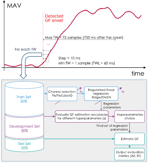
Figure 2. Analysis on the training windows (TW). The upper panel shows the temporal segmentation of the trials into TWs. The bottom panel shows the flowchart of the analysis performed on each of the time segments. Different types of channel selection (Fix/Fix/LassoG) and regularized linear regression (Ridge/EN/EN) were performed for each reduction method under test.
Download figure:
Standard image High-resolution imageSpecifically, to tune the regression parameters and hyperparameters, the TWs extracted from the 240 trials available from each participant were split into training sets (50%), development sets (30%) and test sets (20%). Additionally, the trials that contained the MVC were included in the training set. Then, for each TW, the prediction of the final GF was performed after a selection of channels and/or features using a reduction method. The aim of the reduction method was to obtain sets of 4, 8 or 16 channels and compare the results with those achieved from all HD channels (i.e. 7 × 8 × 3 = 168 channels) to determine the minimum amount of information necessary for the prediction of the target GF. As three reduction methods were compared, this resulted in a total of 12 configurations (4 sets of channels × 3 reduction methods). The three methods used were:
- 1.'Fix-Ridge': the final GF was estimated using a regularized linear regression (with ridge regularization parameter
 {0, 0.001, 0.01, 0.1, 1, 10, 100, 1000}) with a predefined selection of channels (roughly those in the center of the matrices—figure 3) and all the extracted features. This method does not discard any feature.
 - 2.'Fix-EN': solution obtained using the same channels as in the Fix-Ridge method but performing features selection through elastic nets analysis1 [42–44]. A weight parameter α = 0.4 was chosen, whereas different values for the regularization parameter(being λEN the same set of as ) were tested. No limitation on the number and type of features to be retained by the algorithm was included. As a result, the Fix-EN solution could end up with a number of channels lower than the initial value, in the case all features from a channel were discarded. The prediction of the final GF was obtained from the coefficients of the elastic nets.
- 3.'LassoG-EN': solution based on the lasso-group algorithm [45] for automatic selection of the channels, followed by elastic nets for features selection (using the same parameters of the Fix-EN method).


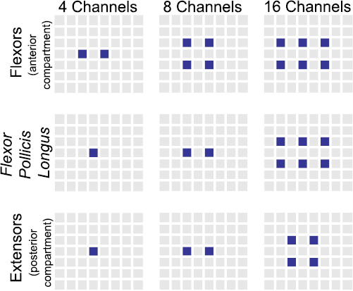
Figure 3. Predefined channels (in blue) for the 'Fix-Ridge' and 'Fix-EN' reduction methods. Each column corresponds to a different subset of channels and each row to the muscle/compartment targeted by the matrix. Anatomically, the matrices were placed having the upper border on the proximal side and the right border on the medial side of the forearm.
Download figure:
Standard image High-resolution imageFor all methods, the algorithms were trained with the training set and the selection of the regularization parameters was based on the performance on the development set while the final assessment was performed on the test set (figure 2, lower panel). Before the training, all features were normalized using the data from the training set. Notably, the chosen step (10 ms), FWL (60 ms) and α (0.4) were identified after preliminary tests using the same dataset split, in order to limit the complexity of the testing. The detailed results of such preliminary tests are omitted here for sake of conciseness2.
The outcomes of the Fix-EN and LassoG-EN reduction methods were analyzed in terms of frequencies and timing of the selected features to get insights about what information was retained after their application.
The R2 and the mean AE calculated as a percentage of GFMVC were used as the metrics to evaluate the estimation of the final GF. Hence, the metrics were also used to identify the TW that optimized the performance of the regression. Specifically, for each configuration and for a subset of TWs (i.e. 300, 350, 400, 450, 500, 550, 600 ms), the difference in AE was analyzed through a Friedman test using R (R Foundation for Statistical Computing, Vienna, Austria). This was followed by post-hoc pairwise comparisons with Bonferroni correction. The TW that exhibited statistically better performance (dubbed TW*) was further analyzed and the frequency of the selected channels was assessed (Fix-EN and LassoG-EN methods).
A two-way repeated measures ANOVA (factors: reduction method and number of channels) with pairwise comparisons was used to identify the overall best configuration. In this case, a single TW, common to all configurations, was used for the comparison. This was chosen as the longest TW among all the TW* selected through the Friedman test. A significance level of p = 0.05 was used throughout the statistical analysis.
On the best configuration selected through the ANOVA, a test comparing the final GF estimation in two additional windows, namely  and
and  , was conducted. The two windows were dimensioned a posteriori considering the average duration of the GF transient across participants. This was done to evaluate the differences in estimating the GF using the transient only with respect to the steady-state only.
3. Results
The recorded data showed that all participants consistently applied final GFs proportionally to the lifted weight. These proved to be (median (inter-quartile range)) 2.9 (1.1), 5.2 (1.2), 7.5 (1.7), 10.5 (1.5)N for the 250 g, 500 g, 750 g, and 1 kg weight, respectively. These corresponded to 7.3 (6.8), 13.7 (9.7), 18.8 (8.3), 23.7 (11.1) % GFMVC, respectively. The GFMVC across participants was 31.1 (16.7)N. The GF onset occurred 69.5 (47.5) ms after the EMG onset. The GF transient lasted 326.3 (186.9) ms.
3.1. Features reduction
The total number of features selected by the Fix-EN and LassoG-EN reduction methods ranged between a couple for small TWs and four channels to a maximum of 150 for larger ones and 168 channels (figure 4(a)—only the case of Fix-EN is displayed). This makes a reduction of the model complexity between 90% and 99%, considering that the initial number of features ranged from 40 (4 channels × 10 features × 1 time sample) to 126 000 (168 channels × 10 features × 75 time samples). Overall the Fix-EN and LassoG-EN mostly retained the following features: WL, TDPSD S, TDPSD IF and dMAV (figure 4(a)). This preference was more visible for shorter TWs, while it attenuated the end of the transient. In addition, the more informative time samples were usually the most recent ones (i.e. the ones at the end of the TW), with the very last time sample in the TW being selected more frequently (figure 4(b)—only the case of Fix-EN is displayed).
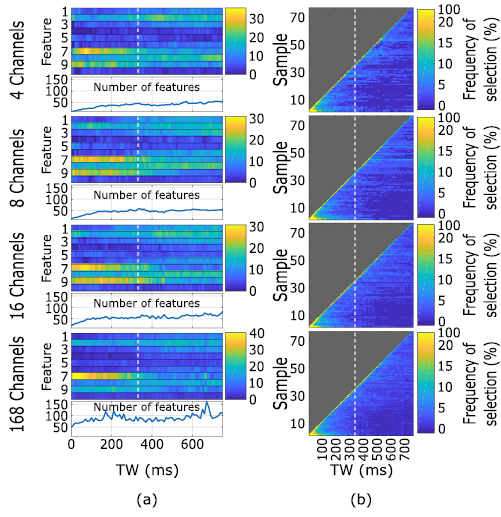
Figure 4. Selection frequency of the time samples and features. (a) Selection of features as a function of the TW length. For each number of channels, the upper colored plot represents the selection frequency of each feature while the lower plot shows the total number of features selected. The features on the y -axis are: MAV (1), WL (2), LogVar (3), vOrder (4), Hjorths Act (5), TDPSD m0 (6), TDPSD S (7), TDPSD IF (8), dMAV (9) and SE (10). (b) Selection of time samples as a function of TW length. Since LassoG-EN and Fix-EN yielded similar results, for the sake of brevity, only the results with Fix-EN are shown. Each row corresponds to a channel configuration. The y axis represents the selected time samples while the x axis represents the TW length. For both (a) and (b), the end of the GF transient is marked by the dotted vertical line. For each TW, the selection frequencies are normalized with respect to the number of features actually selected by the reduction methods.
Download figure:
Standard image High-resolution image3.2. Final GF estimation
In all configurations, the prediction algorithm was able to predict the final grasp force with high accuracy (representative example of the Fix-Ridge reduction method in figure 5). Specifically, the prediction improved according with the TW length, until a stable performance was reached around 400 ms after the GF onset. Notably, as there is little to no EMG activation at the beginning of the transient (TW length close to zero), the performance for the shorter TWs indicates the random guess of the linear regression algorithm. Indeed, under large uncertainty linear regression algorithms return the mean of the target (i.e. the final GF) used during their training [40]. For this subject such value was 6.2 N or 14.7 % GFMVC. Notably, by increasing the number of channels, the estimated GF departs from the random guess even when the TW contains a single sample. The best AE (averaged along TWs length between 450 ms and 750 ms) of this subject was 2.26 % GFMVC.
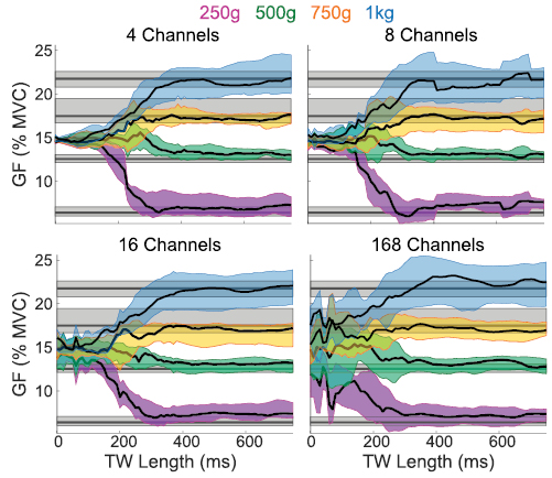
Figure 5. Representative results of the GF prediction. The grey lines correspond to the target GFs while the blue, yellow, green and purple traces correspond to the predicted GFs from the test set of one participant for the 250, 500, 750 and 1000 g, respectively (Fix-Ridge reduction method). The predicted GF is reported for each TW length, which ranged from the moment of the GF onset (1 sample) until 750 ms after it (75 samples).
Download figure:
Standard image High-resolution imageThese results were consistent among subjects and reduction methods. Specifically, all the assessed configurations showed a similar behavior in terms of R2 and AE. The performance improved (R2 increased and AE decreased) with time from the GF onset on, reaching a plateau for TWs of around 450 ms (figure 6). More quantitatively, the R2/AE increased/decreased from 0.1/5% for the shortest TW to 0.8/2% for the longest one (750 ms). When only information from the transient phase was available to the algorithm (i.e. TW = 330 ms) the R2/AE reached a value close to the plateau: 0.67 (0.25)/2.52 (1.76)%. Notably, as there is little to no EMG activation at the beginning of the transient, the performance for the shorter TWs indicates the random guess of the linear regression algorithm. Indeed, under large uncertainty linear regression algorithms return the mean of the target (i.e. the final GF) used during their training [46]. In our problem such value is 7.6 N resulting in an AE of 5.7 % GFMVC.
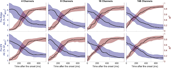
Figure 6. R2 and AE as a function of TW. Each column corresponds to a reduction method. Each row corresponds to a number of channels. The violet plots correspond to the AE and the wine plots to R2, both calculated considering the median across trials per time sample per participant. Solid lines indicate the median and the filled areas the interquartile range. The vertical lines indicate the length of TW* for each configuration (see text for more details). Since LassoG-EN and Fix-EN yielded similar results, for the sake of brevity, only the results with Fix-EN are shown.
Download figure:
Standard image High-resolution imageThe performance of all reduction methods improved slightly as the number of channels increased (figure 6). The TW* were found to be mostly independent from the tested configuration, being either 450 ms or 500 ms (figure 6). Therefore, a TW of 500 ms was considered as the best one in the following analysis.
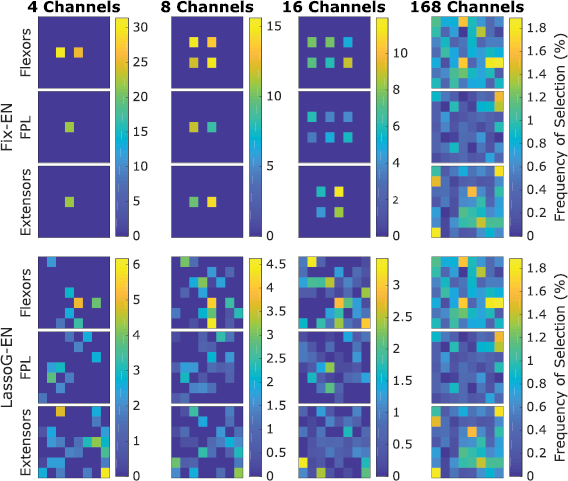
The channels selection frequency (figure 7) showed that Fix-EN, on average, did not discard any channel completely. The most selected channels were usually those from the matrix placed on the flexor muscles. For the LassoG-EN reduction method, the algorithm typically picked different channels for different participants. By definition the 168 channels case reported exactly the same results for both reduction methods.
Figure 7. Channels selection frequency for each HD-EMG matrix for the Fix-EN and LassoG-EN reduction methods, calculated for TW = TW*. Anatomically, the matrices were placed having the upper border on the proximal side and the right border on the medial side of the forearm.
Download figure:
Standard image High-resolution image
3.3. Best configuration
The statistical analysis of the studentized residuals showed that there was normality (Shapiro-Wilk test), no outliers (no studentized residuals greater than ± 3 standard deviations) and no sphericity (Mauchlys test p = 0.002) on the data. Therefore, Greenhouse-Geisser corrections were used. The two-way repeated measures ANOVA showed that the number of channels significantly affected the performance (F(1.83, 18.25) = 16.55, p < 0.001, η2 = 0.71) while the reduction method did not (F(1.35,13.46) = 4.02, p = 0.051, η2 = 0.35). Additionally, there was no interaction between the two factors (F(2.4, 23.96) = 2.12, p = 0.135, η2 = 0.59). Therefore, pairwise comparison was performed on the number of channels only (table 2). This showed that the performance improved when moving from 4 or 8 channels to 168 channels. On the contrary, there was no statistical difference between the 16 and 168 channels configurations, for all reduction methods.
Table 2. Results of the pairwise comparison. The asterisk indicates p < 0.05.
| Mean difference (% GFMVC) | Standard deviation (% GFMVC) | Significance | |||
|---|---|---|---|---|---|
| Fix-Ridge | 4 | 8 | 0.008 | 0.091 | 1.000 |
| 16 | 0.090 | 0.075 | 1.000 | ||
| 168 | 0.310 | 0.123 | 0.183 | ||
| 8 | 16 | 0.082 | 0.056 | 1.000 | |
| 168 | 0.302 | 0.070 | 0.009* | ||
| 16 | 168 | 0.220 | 0.070 | 0.060 | |
| Fix-EN | 4 | 8 | 0.049 | 0.071 | 1.000 |
| 16 | 0.107 | 0.097 | 1.000 | ||
| 168 | 0.372 | 0.109 | 0.041* | ||
| 8 | 16 | 0.058 | 0.083 | 1.000 | |
| 168 | 0.323 | 0.088 | 0.026* | ||
| 16 | 168 | 0.265 | 0.092 | 0.101 | |
| LassoG-EN | 4 | 8 | 0.176 | 0.051 | 0.036* |
| 16 | 0.383 | 0.097 | 0.017* | ||
| 168 | 0.625 | 0.141 | 0.008* | ||
| 8 | 16 | 0.207 | 0.062 | 0.045* | |
| 168 | 0.450 | 0.114 | 0.017* | ||
| 16 | 168 | 0.242 | 0.098 | 0.198 | |
Following these results, the configurations with 16 channels proved the ones with the best tradeoff between complexity and performance. Additionally, as there was no statistical difference between reduction methods, Fix-EN was chosen as the best one due to its reduced computational cost. Thus Fix-EN with a TW of 500 ms was identified as a representative overall best configuration. It allowed for an AE of 1.99 (1.04) % GFMVC which corresponds to 0.64 (0.24)N and to an R2 of 0.82 (0.16).
By analyzing the data from this configuration for each weight separately, the performance in GF estimation seemed to correlate negatively with the weight. Specifically, the mean AE across participants increased from 1.6 (1.05) % GFMVC at 250 g to 1.7 (1.12) % GFMVC at 500 g, 2.4 (1.42) % GFMVC at 750 g and 2.5 (1.23) % GFMVC at 1 kg. Additionally, when evaluating the performance separately for each participant, we found that the AE ranged between 0.71 (1.04) % GFMVC and 4.10 (3.55) % GFMVC.
Finally, to evaluate the differences in performance between transient and steady-state phases, we fixed WTR to the interval 0–330 ms and WSS to 330–660 ms after the onset. This resulted in a median AE of 2.52 (1.76) % GFMVC and 1.75 (1.06) % GFMVC for WTR and WSS, respectively.
4. Discussion
This study aimed at predicting the GF applied while grasping, using salient information extracted from the transient phase of the myoelectric signal. To our knowledge, only one study attempted to extract the GF by continuously estimating muscle force during dynamic changes of the EMG [33]. Specifically, that study tried to determine the force generated by the biceps brachii from a single EMG channel. The authors reported that integration windows of at least 300 ms were necessary to determine the muscle force with acceptable accuracy. As voluntary contractions show faster dynamics, they concluded that the bandwidth of the 300 ms window prevented an accurate continuous estimate of the force. However, in routine grasping a continuous estimation of the GF is probably not needed. Indeed, as with other motor actions, humans grasp in a predictive feedforward fashion, i.e. the final GF is pre-planned and not continuously modulated [47]. Thus, to estimate such a final GF during a functional task (a pick and lift), in this study we adopted a different approach: we used multiple feature samples calculated on shorter (60 ms) time windows.
With this approach, we found that features evaluated using only transient information (TW = WTR = 330 ms) allowed a fair prediction of the final GF with a R2 of 0.67 (0.25) and an AE of 2.52 (1.76) % GFMVC (figure 6). With a 500 ms window we achieved the optimal solution (R2 of 0.82 (0.16) and an AE of 1.99 (1.04) % GFMVC) which in fact was due to the information present in the latter portion of the window (figure 4(b)). In other words, this suggests that the information contained in the steady state is more correlated to the final GF than information contained in the transient phase. Similar outcomes resulted from previous works on transient EMG-based movement classification, in which the steady-state based classification of four and six hand/wrist movements outperformed significantly the transient-based one [48, 49]. While on the one hand this may limit the breadth of this study—the transient contains suboptimal information about the preplanned GF, which is better described by the steady state—it should be considered that the envelope of the EMG (during the steady state) is considered to be a good approximation of the actual GF. However, we argue that finding suboptimal information about the final GF is per se an interesting result, that invites studies where more sophisticated algorithms are assessed to find even better results.
It should be noted that comparing these outcomes with the literature is not straightforward and should be done cautiously. Indeed, no two studies used the same number, type and configuration of electrodes, nor targeted the same muscles or movements nor used the same evaluation metrics (table 1). This being said, comparing our results with others that used the same metrics, our GF predictions on average outperformed previous studies which reported AEs between 4.21 and 12.2% of the GFMVC [22, 23] (table 1). These performances are actually comparable with the ones from the subject that performed the worst in our study (4.10 (3.55) % GFMVC). Concerning the R2, results are comparable with the literature (table 1) reporting values between 0.78 and 0.95 for single movements [9–11, 21, 26, 28] and between 0.90 and 0.93 for simultaneous movements [12, 15, 20, 27]; we argue that the mismatch between AE and R2 results was due to the range of tested weights. Indeed, the GF in this study varied roughly from 5 % GFMVC to 25 % GFMVC whilst other investigators assessed forces from 20 up to 50, 80 or even 100% of the muscle MVC. This wider range found in the literature entails that slight differences in the target forces have a smaller impact on the goodness of fit, yielding higher R2. Conversely, the weights assessed here were all relatively small, making R2 more susceptible to variability. This difference actually influences the AE as well, that is intrinsically smaller due to the smaller weights. However, as the capability to fine tune the GF is more relevant for light and fragile objects, we deemed necessary to use small weights.
While HD-EMG was chosen in order to collect as much information as possible, reduction methods were included to limit the complexity of the problem. Given that, up to our knowledge, there is no consensus about a preferred method, we compared a manual reduction with two approaches with an increasing level of automation. We opted for the elastic nets regularization method because it is less prone than more traditional methods (e.g. sequential features selection or correlation threshold [50]) to the issue of collinearity within features [42] (a known problem in EMG data [37]). To automatically select channels, we adopted the LASSO-group algorithm that allowed discarding all features from the least significant channels within the regularized regression training [45] akin to previous studies [43].
The use of these reduction methods resulted in three main findings. First, when multiple samples are available the most selected ones are the latest available (figures 4(a) and (b)). This suggests that the more we approach the steady-state, the better it is for the final GF estimation accuracy. This is in line with our test involving the two separate windows (WTR and WSS). Results confirm that using transient data the information about GF is available. Specifically, even if the WSS window allows a higher accuracy of estimation, estimations from both windows greatly differ from the random guess. The reduced accuracy in the WTR could be the effect of a lower signal to noise ratio at the beginning of the contraction.
The second finding concerns the features choice. The EN algorithm mostly selected the WL, TDPSD S, TDPSD IF and dMAV, especially for shorter time windows (figure 4(a)). This is in agreement with previous studies that identify WL [16] and TDPSD [51] features as highly informative features to estimate the GF. Surprisingly, the MAV, which is frequently used for proportional estimation of the GF from EMG [3], was not within the set of most used ones. This confirms that the choice of MAV only for GF estimation could be misleading, as reported in previous studies [52].
The third finding is that reducing the number of channels from 168 to 4 or 8 significantly affects the performance of the algorithm, increasing the AE (table 2) whereas using 16 channels the performance does not significantly change. This is in agreement with previous studies [43, 53] reporting that a very large number of channels contains redundant information [43]. As the optimal number of channels changes with different electrode layouts [43, 54], it may be reasonable to expect similar results even decreasing the number of channels. Another interesting point to discuss in this regard, concerns the location of the most selected channels by the LassoG algorithm (figure 7). These channels do not match those used in the Fix approach. Despite this, there is no statistically relevant difference between the performance of the LassoG and the Fix approach. This is in line with previous research suggesting that the redundancy of available information does not call for the need of a very accurate placing of electrodes [54]. However, it is worth noting that, if less information is available, automatic reduction methods may outperform the uniform selection, as reported by Hwang et al, where a single feature was used [43]. Here, given that all tested approaches resulted in similar outcomes (figure 7), we identified the second approach as the preferred one. Indeed, this method does not require the use of HD-EMG hardware and it operates a strong reduction in the number of retained features, making it more suitable for online implementations.
In this study, instead of imposing fixed force profiles (table 1), we opted for the pick-and-lift paradigm. The great advantage of such an approach relies in the fact that even if the movement is performed in a repeatable fashion, it preserves the variability of the natural movement. This represents a methodological strength of the study because, as the same variability could be found in other activities of daily living, we expect that the generalization capability of our solution in clinical settings will be higher than those obtainable by synthetic and highly-controlled experimental tasks.
There are some limitations to this study to be mentioned. First, the study was run in a single session, involved able-bodied participants only and the analysis was conducted offline. In the framework of translating these results to the clinical practice, an online evaluation including both able-bodied and amputees over multiple sessions is necessary to properly evaluate the performance of this method, its stability across sessions and the ability of the subject to improve with practice. Indeed, the important anatomical differences between these two groups would probably affect the performance of the proposed algorithms, or at least require their adaptation. Related to this aspect is the fact that we included information from the FPL muscle. This restricts the target clinical population to very distal amputations (basically wrist disarticulations). Further studies should thus be carried out to understand the relative importance of the information from this muscle on the performance of the proposed method. Another aspect that should be considered in future activities is the detection of the onset. In this study the onset was determined from the GF but this is not feasible in practice and it should be determined from the EMG signals. EMG onset detection is a well-known and non-trivial problem on its own due to the physiological basis of the signal [36]. Thus, as targeting this problem was out of the scope of our study, we preferred to work in conditions in which the variability of EMG onset detection did not influence the outcomes. Nevertheless, to translate our methodology into an online system, an option could be to detect the EMG onset and shift the beginning of the TW according to the average time difference between EMG and GF's onset. This is only one option and foreseen activities will address these limitations in upcoming research.
5. Conclusions
The present work provides a method to detect the final GF exerted on an object from information contained in the transient phase of the EMG. Results show that information about the final GF is already available in the transient phase (0–330 ms after the onset) even if the accuracy of GF estimation can be improved by extending the observation interval up to 500 ms. The importance of estimating the GF during the transient phase relies in the fact that a fast estimation of both the grasp type and the intended grasp force would enable a new generation of myoelectric prostheses with a remarkable usability and responsiveness, with no need of retaining for a long period of time the contraction to control it using the steady state EMG.
The steps to follow in this work will be about the online implementation of the proposed method and its testing with both able bodied and injured patients including a larger vocabulary of grasp types. Such solution will allow us to quantify the improvement in usability of a transient-EMG based solution for GF estimation in a close-to-real use scenario.
Acknowledgments
This work was funded by the European Commission under the DeTOP project (LEIT-ICT-24-2015, GA #687905), by INAIL (the Italian National Workers' Compensation) under the CECA2020 project and by the Italian Ministry of University and Research under the ARLEM project (GA #R16H2KJRHA). The work of CC was partially funded by the European Research Council under the MYKI project (ERC-2015-StG, GA #679820).
Footnotes
- 1
Elastic nets is a regularization approach that merges ridge and lasso regression using a weight parameter α. With α = 1 a lasso regularized regression is obtained, achieving a stronger effect in terms of selection of features; conversely an α approaching to zero leads to a ridge regression that reduces the weight of the features without discarding them.
- 2
In a nutshell, six FWLs (10 ms, 30 ms, 60 ms, 90 ms, 120 ms, 150 ms) were compared. The value of 60 ms yielded the best tradeoff between performance and resulting temporal filtering. Likewise, for the elastic nets analysis, five α values (0.2, 0.4, 0.6, 0.8, and 1) were tested and 0.4 yielded the best performance on the development set.