
Abstract
Objective. To develop and implement a novel approach which combines the technique of scout EEG source imaging (ESI) with convolutional neural network (CNN) for the classification of motor imagery (MI) tasks. Approach. The technique of ESI uses a boundary element method (BEM) and weighted minimum norm estimation (WMNE) to solve the EEG forward and inverse problems, respectively. Ten scouts are then created within the motor cortex to select the region of interest (ROI). We extract features from the time series of scouts using a Morlet wavelet approach. Lastly, CNN is employed for classifying MI tasks. Main results. The overall mean accuracy on the Physionet database reaches 94.5% and the individual accuracy of each task reaches 95.3%, 93.3%, 93.6%, 96% for the left fist, right fist, both fists and both feet, correspondingly, validated using ten-fold cross validation. We report an increase of up to 14.4% for overall classification compared with the competitive results from the state-of-the-art MI classification methods. Then, we add four new subjects to verify the validity of the method and the overall mean accuracy is 92.5%. Furthermore, the global classifier was adapted to single subjects improving the overall mean accuracy to 94.54%. Significance. The combination of scout ESI and CNN enhances BCI performance of decoding EEG four-class MI tasks.
Export citation and abstract BibTeX RIS

Original content from this work may be used under the terms of the Creative Commons Attribution 3.0 licence. Any further distribution of this work must maintain attribution to the author(s) and the title of the work, journal citation and DOI.
1. Introduction
The brain–computer interface (BCI) provides an information exchange and control channel independent of peripheral nerves and muscles for the brain and the outside world. It can directly read the physiological electrical signals in the human brain, analyze their meaning, and convert them into control signals to control external devices. Currently, neuroimaging techniques used in BCI systems commonly include functional magnetic resonance imaging (fMRI), electrocorticography (EcoG), magnetoencephalography (MEG) and electroencephalogram (EEG). EEG has become more and more popular because of its advantages such as low cost, easy portability and high temporal resolution. EEG signals contain sensorimotor rhythms (SMRs) [1–3], slow cortical potentials [4–6], P300 [7–9], and steady-state visual evoked potential [10–12]. Due to its spontaneity and high application value, much attention is paid to SMRs.
In SMRs-based BCIs, the most relevant brain oscillations are found in the alpha (8–13 Hz) and beta (13–30 Hz) frequency bands.[13] The imagination of limb movement produces a unique mode in the SMR. Not only event-related synchronization (ERS) but also event-related desynchronization (ERD) consists of these modes in SMR. A few hundred milliseconds before the start of the exercise, ERD occurs with the energy in the alpha and beta bands dropping rapidly. In the 1–2 s after the end of the exercise, ERS occurs with the beta band energy increasing rapidly. BCIs not only have a positive impact on users with disabilities in terms of life quality and communication with their environment, but also offer new modes of human-machine interaction for both disabled and healthy users such as music generation [14] and computer game control [15]. An increasing number of systems allow control of more sophisticated devices, including orthoses [16, 17], prostheses [18, 19], a robotic arm [20, 21], and mobile robots [22]. In addition, BCIs are also used in aerospace and military applications.
Despite of the fast development of SMR BCIs, there are also various limitations on its classification. The EEG electrodes measure electrical activities on the scalp surface, indirectly providing conclusive location and distribution of the related activated sources which attracts more interests among neuroscientists. Many approaches were proposed to estimate brain source activation patterns from EEG data because EEG sensors cannot measure activated brain sources directly. He Bin and cooperators have studied a BCI approach based on source analysis over the past decade [23–27]. The measured electrical potential can be projected onto a source space by using EEG source imaging (ESI) which consists of modeling electrical activities with current dipoles. Two main approaches, dipole fitting methods [25, 26] and distributed models [23–25, 27] have been proposed for ESI. As ESI performs better than sensor domain analysis in classification of MI tasks, it has gained a great amount of attention.
Also, many methods based on deep learning (DL) were proposed for EEG classification. Kumar et al and Yang et al put forward a suggestion that multilayer perceptron (MLP) was used as a classifier [28, 29]. Dose et al proposed a DL model which used CNN layers for learning generalized features and dimension reduction while using a conventional fully connected (FC) layer for classification, achieving global average accuracy of 68.51% [30]. Chiarelli et al improved BCI performances significantly (two classes: 83.28% ± 2.36%) by employing multi-modal recordings in combination with advanced non-linear deep learning classification procedures [31]. Duan et al used extreme learning machines for improving classification of motor imagery BCI data [32, 33]. Wang et al proposed the methods based on long-term and short-term memory to achieve robust classification [34, 35]. Lu et al developed a method based on Restricted Boltzmann Machines for motor classification [36]. Convolutional neural networks (CNNs) [37] have resulted in a significant improvement in the performance of image recognition, segmentation, detection and retrieval [38–40]. Tabar et al reached high accuracy (two classes:77.6% ± 2.1%) using time-frequency maps from STFT as input to a CNN [41]. Jiao et al built deep CNNs for mental load classification based on EEG data [42].
Although many scholars have made remarkable achievements in this field, there is still a need for accuracy improvement. For MI-based BCIs, the performance of two-class classifiers is stable enough and good, but the classifiers for three or more classes still needs to be improved. Most of these studies are based on sensor domain data instead of source domain data while the source domain contains more information related to MI. Currently, classifiers based on source-domain analysis are targeted at specific subjects with poor generalization performance, thus limiting the application of BCIs.
In this paper, we propose a novel approach via scout ESI and CNN to classify the motor imagery EEG signals. By using scout ESI as our ROI selection method, we propose a novel scout for the MI-EEG. The scout of the most interest is of great importance in several ways. First, it is a part of motor cortex, the most sensitive area for MI tasks, and thus the four MI tasks have the highest discrimination in it. Second, in terms of information content, it enriches the features, and the features extracted from its time series include time, frequency and space information. Third, by combing the scout ESI with CNN, the kernels learned in the networks only pay attention to these features associated with MI tasks, which improve the accuracy of classification. Moreover, the CNN improves the generalization of models. The proposed method has achieved the state-of-the-art performance on Physionet database, significantly increasing the average accuracy.
2. Materials and methods
2.1. System framework
The system framework displays in figure 1. The raw data were recorded from 64 electrodes as per the international 10-10 system (excluding electrodes Nz, F9, F10, FT9, FT10, A1, A2, TP9, TP10, P9, and P10) and sampled at 160 samples per second. Raw EEG was acquired from 64 channels located according to the international 10-10 system and recorded using BCI2000 system. The recorded data were separated into four separate MI tasks including left fist MI, right fist MI, both fists MI and both feet MI. Firstly, the EEGs were bandpass filtered between 8 and 30 Hz using a FIR filter [23], since ERD is distinct in alpha and beta while performing motor imagery. Then, the activity in sensor space was converted into that of source space by computing sources which contain forward and inverse problems. Next, the scouts were created and the features were extracted. We created ten scouts within motor cortex since we were only concerned about motor related activity. Each of the ten scouts represents a region of interest (ROI) in the available source space and is a subset of dipoles defined on the cortex surface or the head volume.[43] Scouts in the left brain are termed as L1, L2, L3, L4, L5 and scouts in right brain are termed as R1, R2, R3, R4, R5. Features were extracted from the source time series of the ten scouts using JTFA. Finally, the time-frequency maps were separated and then classified by the proposed CNN.

Figure 1. The system framework including EEG task separation, EEG preprocessing, source computation, scout creation, feature extraction, frequencies separation and classification.
Download figure:
Standard image High-resolution image2.2. The Physionet database and data preprocessing
This dataset was created and contributed to Physionet [44] by the developers of the BCI2000 [45] instrumentation system which they used in making these recordings. In our work, only the MI trails of ten subjects selected randomly were used (S5, S6, S7, S8, S9, S10, S11, S12, S13, S14). The dataset we used for our analysis consists of 84 trails per subject with 21 trails per class. Subjects performed different motor imagery tasks while 64-channel EEG was recorded. Each subject performed three runs of 21 trails for each of the four following tasks:
- (1)When a target appears on the left side of the screen, the subject images opening and closing the corresponding fist until the target disappears. Then the subject relaxes.
- (2)When a target appears on the right side of the screen, the subject imagines opening and closing the corresponding fist until the target disappears. Then the subject relaxes.
- (3)When a target appears on the top of the screen, the subject imagines opening and closing either both fists until the target disappears. Then the subject relaxes.
- (4)When a target appears on the bottom of the screen, the subject imagines opening and closing both feet until the target disappears. Then the subject relaxes.
To unify the data dimension, we chose 4 s of data because the imagery tasks were performed around 4 s every time. Also, EEG tasks were separated. Left fist, right fist, both fists and both feet MI tasks are termed as T1, T2, T3 and T4, accordingly.
2.3. Source computation based on BEM and WMNE
Tackling the EEG forward and inverse problem is significantly critical to the source computation. To solve the EEG forward problem, brain phantom is carried out which describes the composition, shape distribution and conductivity of brain tissue. Solving the EEG forward problem by using the boundary element method (BEM) [46] generates a lead field which converts the activity from sensor space into that of source space. This association can be represented by the linear system in (1), where R represents the recorded scalp data, L the lead field, N the measurement noise and I the current densities:

Source computation is used to estimate the activities of the thousands of dipoles described by the forward model when only a few hundred spatial measurements are given as input (the number of sensors). To compute sources, the highly underdetermined problem could be solved using L2 norm least squares through (2):

where  is a regularization parameter and W is a weighted matrix. Tikhonov regularizations were also applied to further constrain the solution.
The weighted minimum norm estimation (WMNE) [47] is usually used when the detailed information of the source configuration is unavailable. The lead field and scalp potentials are taken as input, and the estimated cortical current density is provided as an output:

The lead field matrix L in (1) is calculated by BEM, and the weight matrix in (2) is constructed by the hybrid method. In this paper, Colin27 MRI average brain [48], a 3D high resolution, anatomically accurate human brain phantom was used for analysis. The phantom completely covering the brain contains 181 × 217 × 181 voxels. Colin27 exhibits fine anatomical details because of the high signal-to-noise ratio.
2.4. Creation of scouts
Where similar ESI studies have selected a region of interest (ROI) by identifying particular gyral landmarks on subject special cortex models [49, 50], we elected to divide motor cortex into ten scouts to be used as ROI. For the physical processing of the body, there is a topographical correspondence between the different parts of the human body and the different regions of motor cortex area of the brain according to the motor homunculus of Penfield's homunculus [51, 52]. That is to say, the MI of different limbs, such as hands and feet, corresponds to different areas of the motor cortex. So, the ten scouts were selected by dividing the motor cortex into ten regions roughly. Since scouts were created manually, there are some deviations in the position. But the manually defined activity-based scouts for the left and right hemisphere, have here the same size (40 vertices), which allows better comparison [53].
Scouts in left and right motor homunculus are termed as L1, L2, L3, L4, L5, R1, R2, R3, R4, and R5, respectively, as shown in figure 2. Each of the ten scouts was extended to 40 vertices. We have one source only per vertex as this is a source model we used with constrained dipoles orientations. The region L1 corresponds to 40 signals, and so do the other scouts.

Figure 2. Ten scouts. The scouts in the left motor cortex were termed as L1, L2, L3, L4, L5 while the scouts in the right motor cortex were termed as R1, R2, R3, R4, R5. These ten scouts cover areas closely linked to the MI tasks.
Download figure:
Standard image High-resolution imageAfter computing sources, ten scouts were created within the motor cortex, as shown in figure 3. Sources of each of the four tasks (T1, T2, T3, T4) were computed for each of the ten subjects (S5, S6, S7, S8, S9, S10, S11, S12, S13, S14) per task every trail using ESI. For each of the four tasks, every subject performed seven trails (#1, #2, #3, #4, #5, #6, #7) per run. The sources of four tasks with ten scouts for each of the ten subjects at the first trail (#1) were displayed. Then ten scouts' time series were extracted which were used for further analysis.

Figure 3. Creation of scouts after computing sources. These scouts are the regions which are greatly influenced by motor imagination. The color of the brain sources indicate the intensity of current activities, with the red color indicating the most intense current activities.
Download figure:
Standard image High-resolution image2.5. Feature extraction
After the sources were calculated, ten scouts containing 40 sources [43] —which correspond to 40 vertices because of the source model with constrained dipoles orientations we used in this paper—were created within the motor cortex and the time series of the scouts was extracted. R5 scout time series were extracted shown as an example, shown in figure 4. The time series of R5 scout were shown at the right of the figure.

Figure 4. R5 Scout time series extraction. The time series of these scouts including R5 scout were extracted for JTFA.
Download figure:
Standard image High-resolution imageIn this paper, features were extracted from scout time series based on a Morlet wavelet. This wavelet was originally designed at a central frequency  in which its temporal resolution is defined by the full-width at half-maximum (FWHM) of its Gaussian kernel, as seen in (4). The central frequency
  was chosen as 1 Hz, and the FWHM of the Gaussian kernel,
  , was chosen as 3 s. The wavelet's length
  was scaled for remaining frequencies
  by means of (5) for better capturing the varying components of oscillatory activity. The wavelet coefficient was calculated at 0.5 Hz intervals and convolved with the selected waveforms by formula (6). The Morlet wavelet, which has non-orthogonality, is an exponential complex-valued wavelet adjusted by Gaussian, and i in (6) is an imaginary number.


2.6. Data analysis
2.6.1. Proposed CNN Architecture
In the last few years, CNN has managed to achieve superhuman performance on some complex visual tasks like image classification, object detection, and visual tracking. The features which CNN learn are hierarchical composing high-complexity features out of low-complexity, which is more efficient than learning high-complexity features directly. Meanwhile, the features are translationally invariant which is universal to detect the same features in other images. Hence, we propose to use CNN to curb and harness the matter of motor imagery classification.
The model is based on the Deep ConvNet architecture proposed in Schirrmeister et al [54], and consists of a six-layer convolution network with two max-pooling layers and three fully connected layers, as shown in figure 5. The number of the kernel and kernel size were empirically determined based on the values used in Krizhevsky et al [55]. With regard to the Physionet database, at first, we used Deep ConvNet architecture which included four convolutional layers, four max-pooling layers and one fully-connected layer. In consideration of the pooling kernel size (a 2D kernel such as 2 × 2 in our work versus a 1D kernel such as 3 × 1 in Deep ConvNet architecture) and stride size (stride both two for height and width in our work versus stride one for height and three for width in Deep ConvNet architecture), we used two max-pooling layers instead of four empirically to better suit for our data size. Besides, we have tried a different number of convolutional and fully connected layers. While adding more convolutional layers, higher accuracy on the test set was produced. When the number of convolutional layers was greater than six, the accuracy barely stopped growing. Finally, six layers of convolution operation and the three fully connected layers in our paper are the best-performing ones in the experiments. And in section 4.1, proposed baseline model have been evaluated on the database, and we also compared different models with it by taking several techniques to prevent overfitting.

Figure 5. The illustration of the proposed CNN architecture. The model consists of six convolutional layers, two max-pooling layers as well as two fully connected layers. Adam was used as the optimization algorithm for this work.
Download figure:
Standard image High-resolution imageDropout, batch normalization and concatenation deployment are implemented which can lead to faster training of the network, better conservation of information throughout the hierarchical process, and avoids overfitting of the network based on their nature, as stated in table 1. On the other hand, the model without them may be prone to overfitting because the EEG signal has low signal-to-noise ratio and the difference between subjects is large resulting in inconsistent distribution.
Table 1. Implementation details for proposed CNN Architecture.
| Layer | Type | Maps | Size | Kernel size | Stride | Padding | Activation | Parameters |
|---|---|---|---|---|---|---|---|---|
| F2 | Softmax | — | 4 | — | — | — | — | 2048 |
| D5 | Regular dropout | — | — | — | — | — | — | — |
| A7 | Activation | — | 512 | — | — | — | Leaky ReLU | — |
| BN4 | Batch normalization | — | 512 | — | — | — | — | — |
| F1 | Fully-connected | — | 512 | — | — | — | — | 1835 008 |
| Flatten | Flatten | — | 3584 | — | — | — | — | — |
| P2 | Max pooling | 128 | 7 × 4 | 2 × 2 × 128 | 2 | — | 0 | |
| D4 | Spatial dropout | 128 | 14 × 8 | — | — | — | — | — |
| A6 | Activation | 128 | 14 × 8 | — | — | — | Leaky ReLU | — |
| C6 | Convolution | 128 | 14 × 8 | 3 × 3 × 128 | 1 | SAME | — | 147 584 |
| R2 | Concat | 128 | 14 × 8 | — | — | — | — | — |
| A5 | Activation | 64 | 14 × 8 | — | — | — | Leaky ReLU | — |
| BN3 | Batch normalization | 64 | 14 × 8 | — | — | — | — | — |
| C5 | Convolution | 64 | 14 × 8 | 3 × 3 × 64 | 1 | SAME | — | 36 928 |
| D3 | Spatial dropout | 64 | 14 × 8 | — | — | — | — | — |
| A4 | Activation | 64 | 14 × 8 | — | — | — | Leaky ReLU | — |
| BN2 | Batch Normalization | 64 | 14 × 8 | — | — | — | — | — |
| C4 | Convolution | 64 | 14 × 8 | 3 × 3 × 64 | 1 | VALID | — | 36 928 |
| P1 | Max pooling | 64 | 16 × 10 | 2 × 2 × 64 | 2 | — | 0 | |
| D2 | Spatial dropout | 64 | 32 × 20 | — | — | — | — | — |
| A3 | Activation | 64 | 32 × 20 | — | — | — | Leaky ReLU | — |
| C3 | Convolution | 64 | 32 × 20 | 3 × 3 × 64 | 1 | SAME | — | 36 928 |
| R1 | Concat | 64 | 32 × 20 | — | — | — | — | — |
| A2 | Activation | 32 | 32 × 20 | — | — | — | Leaky ReLU | — |
| BN1 | Batch normalization | 32 | 32 × 20 | — | — | — | — | — |
| C2 | Convolution | 32 | 32 × 20 | 3 × 3 × 32 | 1 | SAME | — | 9248 |
| D1 | Spatial dropout | 32 | 32 × 20 | — | — | — | — | — |
| A1 | Activation | 32 | 32 × 20 | — | — | — | Leaky ReLU | — |
| C1 | Convolution | 32 | 32 × 20 | 3 × 3 × 1 | 1 | SAME | — | 320 |
| Input | Input | 1 | 32 × 20 | — | — | — | — | 0 |
In our model, 50% dropout was carried out referring to the drop out of neurons during training. Spatial dropout was implemented after a convolutional layer and regular dropout was deployed after the fully-connected layer. Noticeably, spatial dropout implemented after a convolutional layer meant that the entire 2D feature maps would be removed instead of individual elements, helping to promote independence between feature maps. Concatenation (Concat) was utilized twice to avoid losing features and to maintain the original information, assembling the original layer with the next layer. Furthermore, we used batch normalization after convolutional operations, which was especially useful for fitting the model and improving the accuracy. Given the input  ,
,  is the mean,
  the variance, and
  ,
,  the learned parameters during training. Mini-batch training was used which splits the total training samples into smaller babies and updates all the parameters after learning one mini-batch rather than one single sample. The size of batch we used was 64.


During training, a CNN finds the most useful filters for its task through the Back-propagation Algorithm (BP-Algorithm), and it learns to combine them into more complex patterns. Raw data has been processed directly as the input of CNN by most works while the proposed CNN architecture uses features extracted from source time series using the Morlet wavelet, as shown above.
Besides, in most works, the sampling frequency is correlated closely with the number of channels. However, from the time-frequency maps, it can be found that the sensitivity of each frequency is different for MI tasks, so each frequency is taken as a single sample and the dimensionality of the preprocessed sample is 640. While taking account of the size (both height and width) of output feature maps, the dimension 32 × 20 was empirically chosen when evaluating the networks' metrics in the reminder of this article. Compared with that of 40 × 16 or 64 × 10 which would lead to larger deviation of height and width after the convolution operation, it is computationally infeasible to design the model based on the proposed network hyperparameters, such as the kernel size, stride, and padding.
Furthermore, a large number of experiments that changed the size of the input samples showed that when the input shape of the CNN is 32 × 20, better performance occurs and higher precision is produced.
Each sample corresponds to a label with one-hot encoding that is all zero values except the index of the label marked with a1. The Adam optimizer minimizes the loss function and updates the weights and bias through Back-propagation Algorithm.
Leaky ReLu (Rectified linear units) activation function was used to avoid the problem of gradient vanishing as shown below.

Euclidean distance was utilized as the loss function to measure the divergence between the desired classification model and the proposed method. For this work, the Adam optimization algorithm was used as the optimizer to minimize the loss function using the constant 1 × 10⁻⁵ as the network learning rate.
2.6.2. Classification and evaluation metrics.
Softmax function was employed to predict which task the test data belongs to. The last fully- connected layer outputted four neurons [ ,
,  ,
,  ,
,  ]. The predicted output class
  is defined as follows:

To evaluate the performance of the motor imagery classification, we use the several commonly used metrics including global average accuracy, separate accuracy on each task, macro-precision, macro-recall, and F measure. ROC Curve (Receiver Operating Characteristic Curve) and Precision-recall Curve are utilized to compare the performance of different scouts.


Here, n is total number of categories.  (true positives) is the number of samples assigned correctly to class
  ;
;  (true negatives) is the number of samples that correctly assigned to other classes except class
  ;
;  (false positives) is the number of samples that do not belong to class
  but are assigned to class
  incorrectly by the classifier; and
  (false negatives) is the number of samples that are not assigned to class
  by the classifier but which actually belong to class
  . In macro-averaging, precision and recall is computed locally over each category first and then the average over all categories is taken. Then F-measure for each category
  is computed and the macro-averaged F-measure is obtained by taking the average of F-measure values for each category as:


Macro-averaged F-measure gives equal weight to each category, regardless of its frequency. It is influenced more by the classifier's performance on rare categories. The evaluation metrics above were used to measure the performance of our proposed model.
3. Results
3.1. Time-frequency maps
Features of the scout were obtained using a Morlet wavelet approach. For each task, the time-frequency maps of R5 scout are seen in figure 6. The time-frequency analysis method which contains time and frequency complements provides joint distribution information of the time domain and the frequency domain, and clearly describes the relationship of the signal frequency with time.

Figure 6. Time-frequency maps of the scout R5 for each of the four tasks. The frequency definition is linear, from 8 Hz to 30 Hz and the step is 1 Hz which is of much importance to MI. Joint time-frequency analysis simultaneously describes the energy density or intensity of the signal at different times and frequencies. The color of the time-frequency maps indicates the intensity of energy density, with the red color indicating the most intense energy density activities.
Download figure:
Standard image High-resolution imageObviously, only some parts of the time-frequency maps are red indicating that each task is only sensitive to specific frequencies and time. As the number of the maps is large, CNN is used to choose and learn most essential feature of these maps.
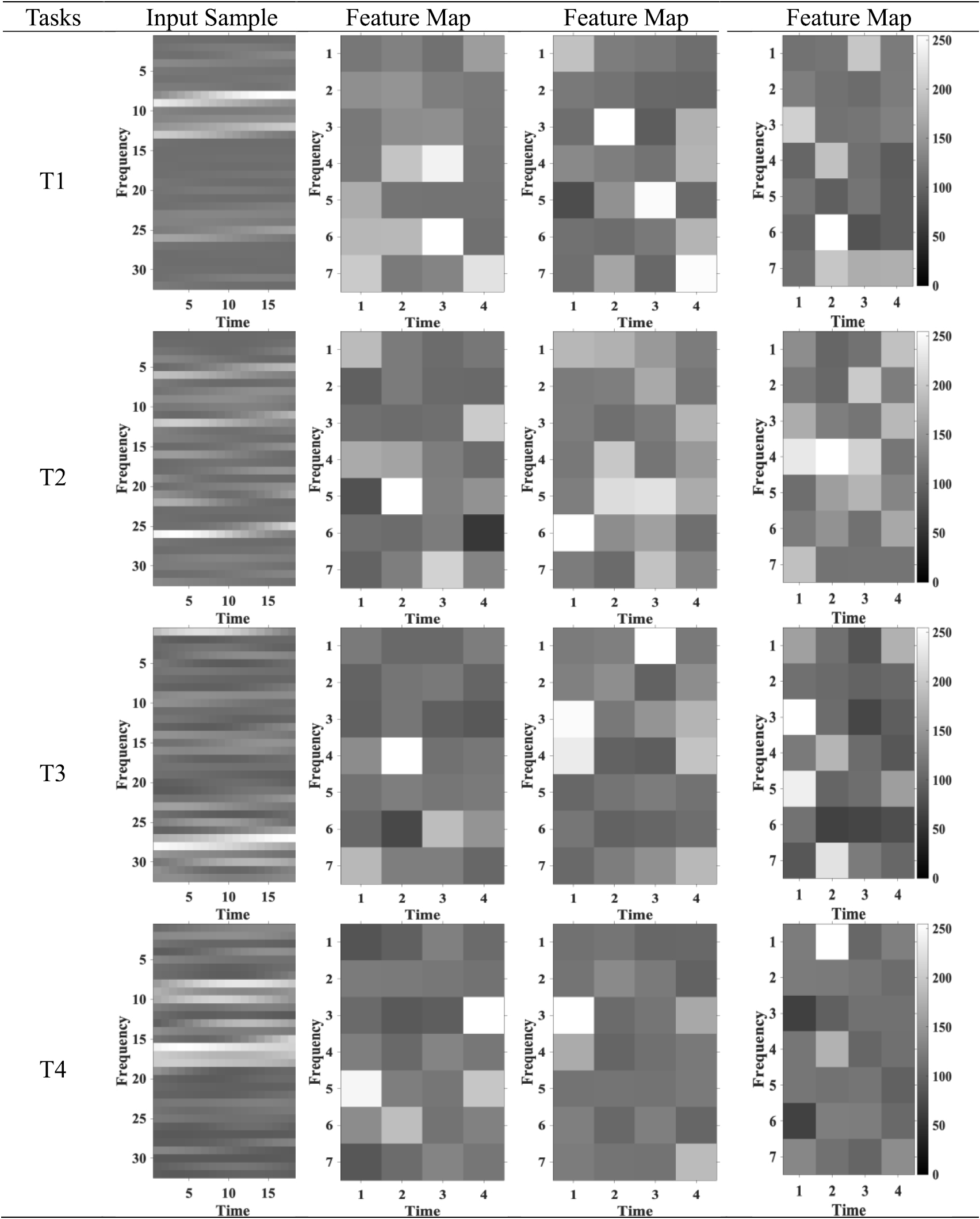
3.2. Feature maps visualization
We randomly selected several samples and visualized some of feature maps as learned representations of MI tasks, in figure 7.

Figure 7. Feature maps visualization of randomly selected samples. Each input sample (32 × 20) corresponds to each task and generates 128 feature maps (7 × 4) after the second max-pooling operation and some feature maps of samples are shown above.
Download figure:
Standard image High-resolution image3.3. Classification accuracy
To obtain valid results, the dataset was separated into 90% as the training set and the remaining 10% as the test set. At first, the dataset of ten subjects (19 320 samples in total) was divided into 17 388 samples to train the proposed CNN architecture and 1932 samples to verify the effective-ness of the model. Moreover, another four subjects' dataset was elected to add up, with the amount of dataset (27 048 samples), in which 24 343 samples were training set and the others were test set.
The proposed CNN architecture was trained and tested ten times on the selected scout to verify the robustness of the proposed model.
The global averaged accuracy of each of the ten scouts is shown in figure 8(a). The  of R5 is the highest, peaking at 94.5% while that of L2 is the lowest, 91.3%. And the corresponding overall accuracies of L1, L3, L4, L5, R1, R2, R3 and R4 are 92.4%, 92.5%, 93.6%, 91.9%, 93.0%, 91.8%, 92.1% and 92.6%. In addition, the overall accuracies all scouts achieved are over 91% and the standard deviations of them are lower than 0.20%. Figure 8(b) shows the group-level statistical results of each of the four MI tasks in each of the ten scouts and the standard deviations of them. T1 achieved the highest accuracy on R5, T2 on R5, T3 on R5, T4 on R1. In general, R5 outperformed than others and L2 did the worst at iteration 2000. The standard deviations are small, indicating that these accuracies are closer to the average and stable.

Figure 8. (a) Global average accuracy of four MI tasks for ten subjects using the source-based methods plotted as a function of the different scouts. The maximum accuracy was achieved when R5 scout was used. (b) Separate accuracy for ten subjects. The peak overall accuracy of T1, T2, T3 was all achieved in R5 scout and that of T4 was achieved in R1 scout.
Download figure:
Standard image High-resolution imageThe confusion matrix with standard deviations is displayed in figure 9(a) illuminating the group-level classification results. T1, T2, T3 and T4 achieved 95.3%, 93.3%, 93.6%, 96.0% at their respective peak global average accuracy. Each of the four MI tasks on R5 scout is shown in figure 9(b).

Figure 9. (a) Confusion matrix for the source-based method at their respective peak overall accuracy. (b) R5 scout seleced for four tasks. The time series of R5 scout were extracted for JTFA as three of the four tasks achieved the highest accuracy in R5 scout.
Download figure:
Standard image High-resolution imageThe performance of the scout R5 was determined by ten tests which changed the order of training and test sets, and the results are shown in figures 10(a) and (b). In ten tests, the mean accuracy of T1, T2, T3, T4 on scout R5 is 93.3%, 93.8%, 94.2%, 94.1%, accordingly. In other words, the mean accuracy of each of the four tasks is over 93%. Also, the global average accuracy is 93.7%. From the results of ten tests, it was found that the classification effect is better on the scout R5. From the results above, it is clear that R5 scout plays the most important role in classifying the four MI tasks.

Figure 10. (a) Global average accuracy on R5 for ten subjects. The maximum and minimum of global average accuracy were achieved in the t10 and the t2, respectively (t10—the 10th test, t2—the 2nd test). (b) Separate accuracy on R5 for ten subjects. T1, T2, T3, and T4 achieved the maximum accuracy on R5 correspondingly at the 10th, 9th, 8th, and 7th tests.
Download figure:
Standard image High-resolution imageTherefore, R5 was selected for the classification of the four MI tasks.
4. Discussion
4.1. Model comparison
As discussed above, the techniques of dropout, batch normalization, and concat are used to address the problem of overfitting in the proposed CNN architecture. Compared with the models without dropout, without batch normalization (BN), without both the dropout and BN, without concat, without both the concat and dropout, without both the concat and BN, without all the techniques, under the results of global average accuracy, separate accuracies on four tasks, and ROC curve of difficult models, given are the experiments' graphs illustrating the effectiveness of the proposed model.
According to figure 11(a), at the early iterations of the models, the percentages of the model with dropout and the model without concat and dropout witness a staggering speed and just over 200 iterations, reach a plateau predominating the performance at approximately 83%. The accuracy of the model without concat and BN is lower than the accuracy of the model without dropout and BN at the first 600 iterations and overtakes it at the iteration of 600 roughly 70%, and subsequently shows a sustained growth increasing to about 82.26%. However, the accuracy of the proposed model shows an upward trend with a peak rate of 94.51%. Meanwhile, the robustness of the model without concat is nearly as excellent as the proposed model, whereas the accuracy of the model without concat, dropout and BN is lower than that of the model without dropout and BN. In terms of global average accuracy, the technology we used did improve accuracy, with concat at 1.76%, dropout at 11.44%, and BN at 10.15%.

Figure 11. (a) Comparison of the global average accuracy of different models. The maximum accuracy was achieved by our proposed model. (b) ROC curve of different models. The proposed model performed better than others. (c) Comparison of accuracy on T1 of different models. (d) Comparison of accuracy on T2 of different models. (e) Comparison of accuracy on T3 of different models. (f) Comparison of accuracy on T4 of different models.
Download figure:
Standard image High-resolution imageThe proposed model has the largest AUC (Area Under Curve) value (0.994), followed by the model without concat (0.993), model without BN (0.973), model without dropout (0.963), model without concat and dropout (0.962), model without concat and BN (0.958), model without dropout and BN (0.924), and model without concat, dropout and BN (0.869), as shown in figure 11(b). As can be seen in figures 11(c)–(f), the accuracies of a proposed model on every four tasks (T1, T2, T3, T4) reach the summit at 94.71%, 93.66%, 95.43%, and 92.80%, respectively. The accuracy of each task has a similar increasing trend. In addition, the accuracy of the proposed model is similar to the accuracy of the model without concat, but the proposed model performs better as the number of iterations increases.
Simultaneously, the accuracies of the model without dropout remain almost equivalent to the accuracies of the model without concat and dropout on four tasks. Moreover, the accuracies of the model without all the techniques on the four tasks maintain the lowest level bottoming at 68.48%, 72.38%, 67.01%, and 69.23% separately. Noticeably, at the terminal of the iterations, the accuracies of each model on every four tasks abide at the level and remain stable, which will be our further research focus to continue to boost the accuracy and undermine the classification error. Overall, the performance results dictate that the used techniques in the proposed model are of great essence to promote the robustness of the model to do the classification tasks.
4.2. Performance comparison
The works of Hyun et al [56], Pinheiro et al [57], Ma et al [58], and Does et al [30] performing the same MI tasks on the same data are compared with our work to verify the effectiveness of our method, as shown in table 2. Our method outperforms the best global and subject-specific models, which shows that ESI enhances the decoding of complex MI tasks and CNN improves the generalization performance of the model. Three subjects (S5, S6, S7) were selected for individual analysis using ten-fold cross validation. And the mean accuracy of each subject is 94.54%, 93.91%, 93.76% for S5, S6, S7, respectively, as shown in table 3.
Table 2. Overview over other works performing four MI tasks on Physionet EEG dataset and comparison to this work's results.
| Work | Training | Max. acc. | Methods |
|---|---|---|---|
| Hyun et al (2013) | Global | 66.65% | CSP-LDA |
| Pinheiro et al (2018) | Global | 74.96% | RNA |
| Ma et al (2018) | Global | 68.20% | RNNs |
| Does et al (2018) | Global | 80.10% | CNN |
| Subject | 86.49% | ||
| This work | Global | 94.50% | ESI CNN |
| Subject | 94.54% |
Table 3. Classification results of individual subjects.
| Subject | S5 | S6 | S7 |
|---|---|---|---|
| Accuracy | 94.54% | 93.91% | 93.76% |
Since EEGs are often of low amplitude and noisy, there is no consistency in the patterns among different subjects and the patterns, but our global cross-subject model performs well with high accuracy. We converted EEGs from sensor domain to source domain and extracted features from the specific scout. It is a reasonable assumption that compared with the sensor domain, different subjects may have smaller differences in the source domain because VC (volume conduction) can give rise to spurious instantaneous correlations between scalp EEG signals and potentially leads to misinterpretation of sensor-space EEG analysis. Another reason may be that the R5 scout plays an important role in all subjects performing these MI tasks. Moreover, CNN can learn generalized features and improve the performance of generalization.
The method we have proposed improves the classification accuracy and stability of the high-dimensional BCIs, and at the same time improves the generalization ability of the BCIs, which can make a BCI no longer only suitable for one person, and is more widely used.
4.3. Repetitive experiment
For the purpose of improving the accuracy of the four-class MI tasks, in this paper, we divided the motor cortex into ten scouts as ROI, extracted the features from the scout time series and used CNN to classify the time-frequency maps of four tasks. Of foremost importance, the accuracy of the four-class MI classification is over 90% using our method from the results above while that of other works is lower than 90%. Four new subjects (S15, S16, S17, S18) were added for analysis so as to verify the validity of the method which means that the data of 14 subjects performing the four MI tasks were used for classification. Also, these data were disordered ten times. For the four-class MI classification, R5 is the best choice as mentioned above. Consequently, the features were extracted from the R5 scout time series for the following analysis.
The global average accuracy of each of the ten times differs from 91.9% to 93.4%, as seen in figure 12(a). The accuracy of each of the four tasks on R5 is displayed in figure 12(b) showing that the accuracy of each of the four tasks is over 90.7% every test. The mean of the global average accuracy is 92.5% and the global average accuracy is over 91.0% every time. For T1, T2, T3 and T4, the average accuracy of the four tasks is 92.3%, 92.6%, 93.0%, 92.2%. At the same time, the accuracy of T1, T2, T3, T4 exceeds 91.3%, 91.1%, 90.7%, 90.9% correspondingly in ten tests. These indicate that the accuracy the four MI classification can achieve is over 91% using the method we proposed for new data through training.

Figure 12. (a) Global average accuracy on R5 for 14 subjects. The overall accuracy was highest in the t7 and lowest in the t5(t7-7th test, t5-5th test). (b) Separate accuracy on R5 for 14 subjects. The accuracy of the ten tests of the four tasks did not fluctuate greatly. (c) F1-score on R5 for 14 subjects. (d) ROC on R5. The AUC of the ten tests almost overlapped, infinitely close to 1.
Download figure:
Standard image High-resolution image
The F1-score of each of the four tasks which is the harmonic average of accuracy and recall is over 90%, as shown in figure 12(c). The value of F1-score on scout R5 is greater than 0.9 for each task tested every time. The ROC curve on scout R5 and AUC display in figure 12(d). As the evaluation criteria, the AUC of each test is approximate to 1, indicating that the model is robust.
The ESI processing was based on Matlab Brainstorm, an open source application for MEG/EEG data analysis and the experiments' results were conducted by the Google machine learning frame-work TensorFlow 1.12.0 and a Nvidia GeForce GTX 1060 GPU with CUDA toolkit 9.0.
5. Conclusion
ESI and CNN were proposed in this study to process four-class motor imagery data. EEG signals were preprocessed, and features were extracted from scout time series. Then these EEG features were given in input to the CNN.
In conclusion, this study for the first time reports the application of scout techniques to select a region of interest and the combination of ESI and CNN for classification of MI tasks. The results demonstrated that these MI tasks can be classified with high accuracy and enhanced through scout ESI and the generalization performance can be improved by CNN techniques. Also, successful integration of these tasks into BCI based on source analysis and CNN can help the subject to self-regulate the state of the brain so that it can be used in everyday life.
The method we proposed greatly improved the accuracy and caused the training to take more time. However, in the near future, we will apply our proposed method in a real-time BCI based on motion imaging with the rapid development of hardware configuration to verify its robustness and efficiency.
Acknowledgments
The authors would like to thank PhysioBank and Brainstorm.