

Abstract
This paper describes the calibration of a high precision AC current measurement device which is required in a system to measure AC voltages up to 800 kV in the frequency range of 10 Hz to 400 Hz. The AC current measurement unit of such a system requires the calibration of the input current in the milliampere range at a frequency of approximately 50 Hz, and all measurements have been made at a suitable frequency of 62.5 Hz. An AC quantum voltmeter (AC-QVM) is used to achieve a traceability chain from DC resistance calibration, when it works as DC quantum standard, and as AC quantum standard for the AC current measurement. All DC and AC measurements needed for one calibration point (one current level) can be done in a rapid sequence within 30 min using the same AC-QVM, such that the combined uncertainty is at a level of 1 μA A−1 (k = 1).
Export citation and abstract BibTeX RIS

Original content from this work may be used under the terms of the Creative Commons Attribution 4.0 licence. Any further distribution of this work must maintain attribution to the author(s) and the title of the work, journal citation and DOI.
1. Introduction
At the Physikalisch-Technische Bundesanstalt (PTB), a precision measurement system for high AC voltages (abbreviated as PS-HVAC) was developed and presented in [1–3]. This system is intended to be used for the German national standard for high AC voltages up to 800 kV in the frequency range of 10 Hz to 400 Hz with an overall uncertainty of 25 μV V−1 (k = 1; throughout this paper the uncertainties are always expressed for that coverage factor). It is based on the measurement of a 50 Hz loading current of a high voltage capacitor, and the analogue conversion of this current to a reference voltage. Traceable 50 Hz (or nearby frequency) currents from 0.33 mA to 15 mA are required for calibrating the instrument within its seven measurement ranges. The requirement is to make a current calibration with an uncertainty better than 10 μA A−1.
The AC quantum voltmeter (AC-QVM) based on a programmable Josephson voltage standard (PJVS) has been developed and established at PTB as a system for precision DC and AC voltage measurements for frequencies up to the kilohertz range with amplitudes up to 10 V [4, 5]. Further extensions of AC-QVM applications have been demonstrated including AC and DC resistance comparisons and current measurements [6–8].
This paper demonstrates the use of an AC-QVM in the traceability chain (see figure 1) for convenient and fast calibration of a high-voltage measurement system, like the PS-HVAC. The first results are given in [9]. The calibration procedure includes the calibration of DC reference resistors at DC current, then calibration of AC shunts at DC current, and the calibration of AC currents by measuring voltage drops on AC shunts. AC measurements presented here have been done at a frequency of 62.5 Hz because this frequency is suitable as a working frequency of the AC-QVM but is also close enough to the mains frequency (50 Hz) to ensure that obtained results are valid. All standards (resistance standards, AC shunts) used were kept in a stable thermal condition, the so-called 'warm state'. At least 1 h before performing measurements they were heated with the same current at which the calibration was performed later to avoid drifting due to temperature transients and associated influences. A stable DC current source (marked as DCCS in figure 4) or an AC current source (marked as ACCS in figure 5) is required, and it must be phase synchronised with the AC-QVM for AC measurements.

Figure 1. Traceability chain for the calibration of AC current supplied to the PS-HVAC as device under test.
Download figure:
Standard image High-resolution imageFor the first time the advantage of the AC-QVM to instantly switch from precision DC to AC measurements has been exploited. On one hand, the precision 8.5-digit voltmeters are capable to achieve uncertainty in sub-µV V−1 range for DC calibrations at 100 mV levels, but only cover this amplitude range for AC calibrations with uncertainties of several µVV−1 [10, 11]. On the other hand, AC–DC transfer standards can achieve better uncertainties for AC current measurement, but require longer measurement times [12], so the traceability chain might suffer from the associated higher drift of the AC shunts.
This paper is organized as follows: first, in section 2, we will briefly introduce the DUT (PS-HVAC) and the AC-QVM (because they are presented in detail elsewhere) together with the measurement set-ups used for DC and AC calibrations. In section 3 we will present the measurement results and put them in relation to estimated uncertainties. Finally, a summary and outlook are given in section 4.
2. Measurement set-up
2.1. PS-HVAC current measuring system
The PS-HVAC measuring system consists of an operational amplifier (OPA)-based current-to-voltage converter, precision resistors in each of its seven measurement ranges (marked as '100 Ω' up to '10 kΩ'), a digitizer, and a laptop running a LabVIEW program, forming a measurement unit (figure 2). The PS-HVAC is based on the Chubb–Fortescue method, but the loading current of the high voltage capacitor is converted into a proportional voltage. Since the current of the capacitor is a direct derivative of the high voltage, the measurement signal must be integrated. Here, a software-based integration is used with careful attention to the initial conditions.
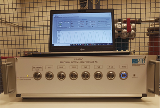
Figure 2. The PS-HVAC measuring system installed in the high voltage laboratory. Seven ranges marked as '100 Ω' up to '10 kΩ' are visible on the front panel of the instrument and can be selected by a laptop running a LabVIEW program.
Download figure:
Standard image High-resolution imageThis system has been developed for calibrations of currents in the milliampere range at a frequency of 50 Hz. However, the system was characterized for measurements of signals with frequencies from 15 Hz to 400 Hz using a sinusoidal current in the range of 0.5 mA to 50 mA, which is the typical loading current of compressed gas high voltage capacitors with values up to 500 pF [1]. The targeted overall relative uncertainty of the entire system, including the HV capacitor, is 25 μV V−1 so the requirement is to make current calibration with a relative uncertainty better than 10 μA A−1. Since the low voltage side of HV capacitor is directly connected to the input of OPA, the influence of the connecting coaxial cable should be negligible on current measurement. The characterization of the individual components has been described in detail [1, 2].
Calibration of the PS-HVAC system means applying a precisely known reference current, measured by AC-QVM, and comparing the current reading on the display of the system (i.e., measured current). Internally measured current is calculated from the voltage drop (and the associated ADC voltage reading) on the precision resistance (with the known nominal value for each range). Therefore, calibration means the determination of the relative correction for measured current cI , expressed in μA A−1 (see results given in table 3) and to be stored into the control LabVIEW program, until it is equal to the reference current. The same procedure should be repeated for each of seven measurement ranges (i.e., at least seven corrections cI should be determined), while the calibration at one particular range can be done with different currents (see results given in table 3). In ideal case, the relative correction for one range should remain constant regardless of the current level used.
2.2. AC quantum voltmeter
The AC-QVM and its extension to a quantum calibrator are discussed in detail in [5, 6], while the schematic of this floating device is given in figure 3, in a setting for AC measurements. The essential part, the PJVS, can generate stable and quantized DC voltages, or stepwise approximated sine waves for frequencies up to the kilohertz range. For DC voltage measurements the AC-QVM is used as common DC Josephson array voltage standard and generates quantized DC voltage up to 10 V. The voltage difference between the voltage generated by the PJVS and the voltage drop on the resistor is measured by an Agilent 3458A 3 voltmeter on its lowest measuring range 100 mV (the resistor and the voltmeter 3458A are not shown in figure 3).

Figure 3. Schematic of the AC-QVM—explanations are given in the text.
Download figure:
Standard image High-resolution imageFor AC voltage measurements, there are two important features which are essential for the correct use of AC-QVM. The first feature is the synchronization between synthesized waveform (stepwise approximation of sine wave), the measured AC voltage and sampler, while the other one is the grounding point defined at the outer BNC connector of the input of a fast sampler (PXI NI 5922 3 ) which operates on power mains. This sampler is used to digitize the difference voltage and it operates with the 1 MΩ differential input. The 48-tap standard finite impulse response filter is selected. A Keithley 3390 50 MHz arbitrary waveform generator is used to set the phase shift between the synthesized waveform and the measured AC voltage by locking its output for the chosen phase difference (details are described in [5]). For AC measurements, the following setting is made (expressed for the completeness of information and chosen as an optimal set-up): a frequency of 62.5 Hz, 20 Josephson steps per period and 4 MSa s−1 sample rate for the sampler. To cut out the transients from the synthesized waveform 200 readings are deleted on both sides of the transients. Typically, 30 periods are measured in a loop (0.48 s) for one RMS value, and then averaging RMS values during one to two minutes is performed. Further details are described in [5].
2.3. DC measurement set-up
The DC set-up is given in figure 4. During DC measurements a Fluke 5720A calibrator 3 (DCCS) is set on voltage output (as we only investigate small currents) and is left floating, while the grounding point is set in the middle point of two resistors.

Figure 4. Measurement set-up schematics for DC measurements. The AC-QVM is connected in an ABBA time sequence to measure the voltage drops on the resistors RDC and RSh. Exchange of the position from A to B and vice versa is done manually.
Download figure:
Standard image High-resolution imageFor this resistance comparison at DC current, the AC-QVM is used as common DC quantum standard, and it measures the voltage UDC on the reference resistor RDC, and after that the voltage USh on the shunt resistors RSh, in a time series with manual reconnection, including four sequences altogether with different polarity of the PJVS voltage and current flow. Finally, the DC resistance of the AC shunt RSh is obtained:

The AC shunt RSh (in our case a Fluke A40B 3 for 1 mA, 10 mA, and 20 mA, as appropriate; see data in table 1) [13] is compared to reference resistors RDC (Fluke 742A 3 −10 k, −100 k or −1 k). These reference standards were chosen due to their robustness (because they are rigid and compact for easy handling), loading capabilities (to handle the relatively high currents) and very small temperature coefficients (which means they could be used at room temperatures without insertion in specially developed thermostat); their characteristics are given in table 2. In the application of RDC in this experiment, the current level for chosen particular reference resistor was held below the maximal DC current to maintain the specified accuracy value, IDCACC, to avoid additional uncertainty contribution due to its self-heating; the exception is only one measuring point at 6.5 mA when Fluke 742-100 is used (which is relatively little higher than 5 mA).
Table 1. Used AC shunts for AC currents from 0.35 mA to 15 mA: Rnom is the nominal resistance and Unom is AC voltage generated for selected measured current. Their temperature coefficients are: |a| ⩽ 0.06 × 10⁻⁶ K−1 and |b| ⩽ 0.05 × 10⁻⁶ K−2.
| Shunt | |||
|---|---|---|---|
| IAC/mA | Type | Rnom/Ω | Unom/V |
| 15 | Fluke A40B-20mA | 40 | 0.6 |
| 8 | 0.32 | ||
| 6.5 | Fluke A40B-10mA | 80 | 0.52 |
| 3.3 | 0.264 | ||
| 1.6 | 0.128 | ||
| 0.8 | Fluke A40B-1mA | 800 | 0.64 |
| 0.35 | 0.28 | ||
Table 2. Resistors used as reference: Rnom is the nominal resistance, IDCMAX the maximal DC current, and IDCACC the maximal DC current to maintain the specified accuracy.
| Reference resistor—type Fluke 742A | |||
|---|---|---|---|
| Type | Rnom/Ω | IDCMAX/mA | IDCACC/mA |
| 742A-10 | 10 | 100 | 20 |
| 742A-100 | 100 | 20 | 5 |
| 742A-1k | 1000 | 10 | 2 |
2.4. AC measurement set-up
The frequency dependence of the shunt resistance is almost negligible for such coaxial current shunts. For the frequency range from DC up to 62.5 Hz it can be assumed that it is <0.3 μA A−1, as shown by the experimental results given in [7], but also from other analysis even for higher currents and/or higher frequencies [14–18]. Therefore, the same shunt can be used for AC measurements, using the value RSh obtained in (1) as its resistance value (figure 5). The AC-QVM measures the voltage USh, while the current IAC for calibrating the PS-HVAC is equal to:


Figure 5. Schematic measurement set-up for AC current measurements. Calibrations of the PS-HVAC were performed with a short cable A. To verify influences of the PS-HVAC on the AC-QVM reading and of a 25 m long connecting cable measurements with connection schemes B and C have made and are discussed later.
Download figure:
Standard image High-resolution imageThe outer pin of the digitizer input connector defines the grounding point of the measurement set-up as the digitizer. In this configuration the Fluke 5720A calibrator (ACCS) is set on the current output. For simultaneous measurements of the AC current, it is essential that the connection of the shunt RSh and the PS-HVAC in series does not cause a problem for the AC voltage measurement by the AC-QVM due to grounding or synchronisation. To verify influences of the PS-HVAC on the AC-QVM reading and cable reflections due to a 25 m long connecting cable measurements with connection schemes B and C (see figure 5) have been made and are discussed in section 3.3. The best calibration results were obtained, and were possible, with simultaneous AC current measurements by both AC-QVM and PS-HVAC, and the control notebook of the PS-HVAC powered on battery. Such setting was not possible with the shunt Fluke A40B-1mA which uses an amplifier that must be powered all the time. In that case the measurements were done successively.
3. Measurement results
The standard calibration procedure consists of the calibration of the shunt, for instance a Fluke A40B-10mA, with reference resistor Fluke 742A-100 at DC current (80 Ω:100 Ω ratio). Then the freshly calibrated shunt itself is used as the reference for calibration of the PS-HVAC at AC current directly afterwards. The chosen current levels were in accordance with the requirements on the calibration of the PS-HVAC system and the available equipment.
In the following subsections examples of the measurement results are given, obtained at different parts of the traceability chain. This has been made in a bid to determine the influencing effects on the results and achievable uncertainties with the equipment used. It starts with the comparison at DC current (subsection 3.1), firstly of two reference resistors and then of AC current shunts with reference resistor. Followed by the AC current measurements using AC shunts (subsection 3.2), and finally the calibration of the PS-HVAC system using AC shunts (subsection 3.3). In all figures in this chapter the error bars correspond to standard deviations.
3.1. DC comparisons of resistances
The reference resistors RDC used at DC measurements are Fluke type 742A (table 2) with their predicted resistance values. These standards were calibrated before this measurement campaign against a quantum Hall resistance using a cryogenic current comparator (see figure 1) with a relative uncertainty of 0.15 μΩ Ω−1 [19–21], that can be assigned to such a type of resistor. To verify our DC calibration procedure (figure 4) and the calibration values for these resistance standards we performed DC comparisons of them. An example of such a 1:10 ratio measurement using Fluke 742A-100 and 742A-1k resistors is given in figure 6. Each measurement point represents one complete measurement set during a time interval of 5 min i.e., each measurement contains four 1 min sequences with different PJVS voltage and current polarities. A ratio can be measured with a type-A uncertainty of 0.2 × 10⁻⁶ for a current of 0.9 mA. If the current is halved to 0.45 mA, the type-A increases to about 0.45×10⁻⁶. It can be seen from the results that the stability of the determined ratio of about 0.15 × 10⁻⁶ for the same current can be expected without many measurement repetitions.
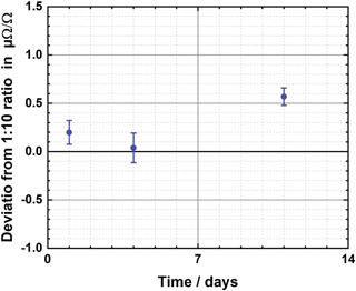
Figure 6. Measurement of the 1:10 resistance ratio at DC, for the 100 Ω and 1 kΩ reference resistors, relative to their nominal ratio. The first and third results are obtained with a current of 0.9 mA, while the second result with 0.45 mA.
Download figure:
Standard image High-resolution imageIn figure 7 the results of the DC calibration of a Fluke A40B-10 mA shunt are shown (as relative errors to a nominal value of 80 Ω) for currents 1.6 mA, 3.3 mA and 6.5 mA using a Fluke 742A-100 as reference. It is obvious from the results that the current dependence is an issue which must be taken into account, i.e., the calibration should be performed at the same current level used for the calibration of the PS-HVAC. The relative experimental standard deviation of the measured shunt resistance of one measuring sequence is 0.26 μΩ Ω−1 at 1.6 mA, 0.13 μΩ Ω−1 at 3.3 mA and 0.07 μΩ Ω−1 at 6.5 mA.

Figure 7. Current dependence of an 80 Ω AC shunt at DC.
Download figure:
Standard image High-resolution imageFor comparison, when calibrating a Fluke A40B-20 mA shunt, it can be as low as 0.24 μΩ Ω−1 for a 15 mA current, while for a Fluke A40B-1 mA shunt as low as 1.1 μΩ Ω−1 for a 0.35 mA current.
3.2. AC current measurements using AC shunts
The stability of an AC current measurement at 62.5 Hz using a Fluke A40B-10mA AC shunt at 3.3 mA is given in figures 8(a) and (b) and in different ways, as explained below.
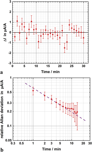
Figure 8. (a) Stability of the AC current measurement at 62.5 Hz and 3.3 mA. An Allan analysis of the data is shown in figure 8(b). (b) Overlapped Allan analysis [22] of the data (figure 8(a)) shows that after about 4 min a relative uncertainty better than 0.3 μV V−1 can be achieved.
Download figure:
Standard image High-resolution imageIn figure 8(a) the differences (as relative errors) between a measured value and the mean value of the 30 min interval are given and marked with ΔI. Each point represents the result of a one-minute measurement started every minute again. Average values for five repeated points obtained in that way have a typical standard deviation of 0.5 μA A−1, while for continuous measurement (without starting the measurement after every minute again) could be even lower. This means that the calibration of the AC current can be done within the time interval of a few minutes with satisfying uncertainty, and this is pointed out in figure 8(b), where the relative Allan deviation is given for such measurement sequence, showing that, after about two to 5 minutes, a relative uncertainty of (0.2 to 0.3) μV V−1 can be achieved.
3.3. Calibration of the PS-HVAC system on different ranges using different AC shunts
As an example, the calibration of the PS-HVAC calibration on the 2 kΩ range at 1.6 mA is described here, and summarised results are given in table 3. In the first two columns, the reference AC current IAC, measured by AC-QVM according to (2), and associated relative standard deviation of the mean sx are shown; in the last four columns there are data relevant to the PS-HVAC: measured AC current IHVAC, associated relative standard deviation of the mean sx , relative error eI of the measured current. In the last column, the relative correction for the measured current cI is given. This is the correction which should be applied to the PS-HVAC as the value obtained through this calibration process; all relative values are expressed in μA A−1. A Fluke A40B-10mA shunt, that is calibrated at DC current with a Fluke 742A-100 reference standard, is used. After the first measurement, the relative correction cI is calculated and adjusted, and such iterative process is repeated until the error eI falls within ±0.5 μA A−1. Before continuing with the next calibration point, usually two more readings were taken to confirm that the satisfied stability is ensured. The final correction cI at this calibration point is 43.0 μA A−1; this result is given in table 4, too.
Table 3. An example of the PS-HVAC calibration on the 2 kΩ range at 1.6 mA—further explanations are given in the text; the value of interest is the relative correction for measured current cI in the last column.
| AC-QVM | PS-HVAC | ||||
|---|---|---|---|---|---|
| IAC/mA | sx /(μA A−1) | I HVAC /mA | sx /(μA A−1) | eI /(μA A−1) | c I /(μA A−1 ) |
| 1.599 999 | 0.14 | 1.599 930 | 0.21 | −43.39 | 0.0 |
| 1.599 999 | 0.25 | 1.600 003 | 0.56 | 2.30 | 45.0 |
| 1.600 000 | 0.15 | 1.599 999 | 0.28 | −0.36 | 43.0 |
| 1.600 000 | 0.17 | 1.599 999 | 0.20 | −0.38 | 43.0 |
| 1.599 999 | 0.15 | 1.599 999 | 0.27 | −0.27 | 43.0 |
Table 4. Results of the PS-HVAC calibration on all ranges—further explanations are given in the text.
| DC Ref. | Measurement by AC-QVM | Settings on PS-HVAC | |||
|---|---|---|---|---|---|
| Fluke 742- | Fluke A40B- | IAC/mA | Range | Percentage of full scale | cI /(μA A−1) |
| 10 | 20mA | 15 | 100 Ω | 50% | −81.0 |
| 8 | 30% | −81.0 | |||
| 15 | 200 Ω | 100% | 64.0 | ||
| 8 | 50% | 66.0 | |||
| 100 | 10mA | 6.5 | 500 Ω | 100% | 141.2 |
| 3.3 | 50% | 141.2 | |||
| 1.6 | 30% | 142.0 | |||
| 3.3 | 1 kΩ | 100% | 145.0 | ||
| 1.6 | 50% | 147.0 | |||
| 1k | 1mA | 0.8 | 30% | 147.0 | |
| 100 | 10mA | 1.6 | 2 kΩ | 100% | 43.0 |
| 1k | 1mA | 0.8 | 50% | 43.0 | |
| 0.35 | 5 kΩ | 50% | 89.0 | ||
| 0.33 | 10 kΩ | 100% | 103.5 | ||
The overall calibration results for the PS-HVAC on all ranges are given in table 4, where the procedure to obtain the relative correction for measured current cI at one calibration point is the same as explained for the results presented in table 3. In the first column of table 4 the reference resistor of type Fluke 742 used at DC measurements is given, in the second column the AC shunt of type Fluke A40B used for AC measurements is given, while in the third column the reference AC current used for calibration is shown. In the fourth, fifth and sixth columns the data related to PS-HVAC are given: selected range, utilization (expressed as percentage of the full scale), and determined cI , respectively. The presented results are very satisfactory and representative even though obtained within the limited time and as first experience. We expect that a repetition of such exercise could lead to even better results.
In ideal case the values of cI should be zero. If that is not the case, as obvious from the results given in table 4, this can be expressed as 'gain error' of the PS-HVAC on its selected range. Furthermore, the values of cI obtained at different current for the same range (for instance, at 30%, 50% and 100% of full scale) should be the same. If this is not the case, the differences can be expressed as 'linearity error'. The obtained results show that such linearity error (if it exists) is comparable to the measurement uncertainty (see table 5). It is also worth to notice that the calibration on the 2 kΩ range, where the same values of cI are obtained at 50% and 100% of full scale, were achieved by using two different reference resistors for the DC measurements and two different shunts for the AC measurements. Such an agreement raises the overall confidence in the calibrations and the PS-HVAC traceability chain. Furthermore, it emphasizes the possibility of the application of the AC-QVM for fast, accurate and traceable precision DC to AC measurements.
Table 5. Uncertainty analysis of the measurement, given for different nominal current levels; all uncertainties are relative ones and expressed in μA A−1.
| IAC/mA | ur(δIref) | ur(δISh) | ur(δIACDC) | ur(δIRMS) | ur(δICAL) | u cr ( I CAL ) |
|---|---|---|---|---|---|---|
| 15 | 0.23 | 0.40 | 0.30 | 0.37 | 0.50 | 0.83 |
| 8 | 0.23 | 0.39 | 0.30 | 0.36 | 0.50 | 0.82 |
| 6.5 | 0.23 | 0.21 | 0.30 | 0.33 | 0.50 | 0.74 |
| 3.3 | 0.23 | 0.20 | 0.30 | 0.39 | 0.50 | 0.77 |
| 1.6 | 0.23 | 0.18 | 0.30 | 0.56 | 0.50 | 0.86 |
| 0.8 | 0.23 | 0.25 | 0.30 | 0.67 | 0.50 | 0.95 |
| 0.35 | 0.23 | 0.76 | 0.30 | 0.41 | 0.50 | 1.07 |
The results presented in tables 3 and 4 were obtained when the reference current feeds directly to the input of the PS-HVAC system. However, for the use in the high voltage set-up, it is necessary to connect the PS-HVAC with the 25 m long coaxial cable, and the evaluation of the influence of such cable on the calibration results is necessary. Furthermore, the influence of the PS-HVAC on the calibration using the AC-QVM must be evaluated (see connections schemes B and C of figure 5), too.
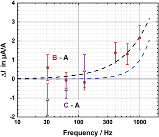
Thus, a measurement of the frequency dependence for the Fluke 5720A 3.3 mA output current on the ACI range from 31.25 Hz to 1 kHz using the shunt Fluke A40B-10mA is presented in figure 9. ∆I is the relative difference for the two cases: (A) with and (B) without the connection of the PS-HVAC system in series with RSh (see connections in figure 5). An additional load could cause a linear frequency behaviour which is fitted by the black dashed line in figure 9. The differences at 62.5 Hz and 125 Hz are at a level of −0.1 μA A−1 and −0.2 μA A−1, respectively.
Figure 9. Frequency dependence of the error ΔI for frequencies up to 1 kHz as a difference between the two cases: (A) with or (B) without connection of PS-HVAC system in series with AC shunt (red points) and frequency dependence of the error current ΔI due the 25 m long coaxial cable connected at the input of the PS-HVCS (see C and A in figure 5). The dashed lines indicate linear and quadratic fits with frequency as explained in the text. The error bars indicate type-A uncertainties (k = 1).
Download figure:
Standard image High-resolution image
The error of the output current ΔI, measured with the PS-HVAC system with (C) and without (A) the 25 m long coaxial cable connected in series, is performed, and their differences are also presented in figure 9. The frequency was varied from 31.25 Hz to 125 Hz, again with Fluke 5720A calibrator used as AC current source. As the differences of both measurements agree well within 1.1 μA A−1 we can conclude that the connection of PS-HVAC and the long cable, cases (B–A) and (C–A), have a negligible influence at 50 Hz. The blue dashed line shown in figure 9 indicates a quadratic fit which is well-known from cable error investigations in a measurement loop. The fit is based on typical numbers from [23] and by taking the 25 m long cable into account. The result shows that such an error should be very small at a frequency of 50 Hz.
In table 5, the input quantities and analysis of their uncertainty contributions are shown, and the relative combined standard uncertainty of the calibrated current is calculated as follows:

The input quantities are: δIref—comparison of the reference resistance standards at DC current, which includes the uncertainty of the used reference and its time stability; δISh—calibration of the AC shunt at DC current; δIACDC—AC–DC difference for the used AC shunt; δIRMS—measurement of the AC current using an AC shunt and the AC-QVM; δICAL—residual contribution of the PS-HVAC calibration due to the set-up and measurement procedure. All given standard uncertainties and combined uncertainty are expressed as relative values in μA A−1. Further uncertainties from the AC-QVM are at a level of 10−8 for AC calibrations [24] and even better for DC calibrations [5, 6] and can be neglected here.
4. Conclusion
We presented the application of the AC-QVM for the establishment of a traceability chain, starting from DC resistance calibration followed by a calibration of an AC shunt at DC current, to an AC current calibration used for the calibration of the PS-HVAC system at 62.5 Hz. DC and AC measurements are done in a time series, maintaining the conditions as stable as possible, and with the used equipment and measurement methods the combined standard uncertainties can be as low as 1 μA A−1 for measured AC currents from 0.35 mA to 15 mA.
All these data demonstrate the potential of the AC-QVM application, which can be used for DC and AC voltage and current measurements, as well as for resistance ratio measurements and for the calibration of complex systems used for high voltages, where the measurements can be done in a short period of time and low level of uncertainty.
Acknowledgments
We acknowledge the support from M Schmidt, M Brennecke, C Rohrig and B Schumacher from PTB for letting us borrow AC and DC resistance standards. This work was co-funded by the EMPIR joint research project 17RPT03 DIG-AC. The EMPIR initiative is co-funded by the European Union's Horizon 2020 research and innovation programme and the EMPIR Participating States. D Ilić would like to extend his gratitude to the PTB colleagues for their continuous support.
Footnotes
- 3
Identification of commercial equipment does not imply an endorsement by FER-PEL and PTB nor that it is the best available for the purpose.