

Abstract
High-accuracy length measurements of prismatic bodies (e.g. gauge blocks) are usually performed by means of single-ended interferometers. To perform these measurements, the gauge block must be wrung to a reference plate. The quality of contact affects the measured length and also the wringing process wears down or damages the measuring faces. Furthermore, it limits the use of such interferometers to bodies that are suitable for wringing. PTB's double-ended interferometer allows high-accuracy length measurements that are traceable to the International System of Units to be performed without a reference plate. However, because the setup of this interferometer is complex and additional optical components are required the alignment process is challenging. Compliance with the defined gauge-block length in ISO 3650 is also challenging, especially for non-perfect shaped gauge blocks. In this work, we develop a precise alignment method for the double-ended interferometer and systematically study the contributions of misalignments to the uncertainty of the measured length. In order to explore the accuracy of the developed procedure and to estimate the size of the uncertainty caused by deviations from perfect gauge block shapes, virtual experiments are carried out using the PTB library SimOptDevice. The virtual experiment is validated by a comparison to experimental data. In addition, theoretical relations are confirmed. Finally, Monte Carlo runs of the virtual experiment are performed to quantitatively explore the size of different sources of uncertainty on the developed alignment method. The results suggest that the developed alignment method is highly accurate and is expected to yield an uncertainty contribution to the final length measurement in the sub-nanometer range.
Export citation and abstract BibTeX RIS

Original content from this work may be used under the terms of the Creative Commons Attribution 4.0 licence. Any further distribution of this work must maintain attribution to the author(s) and the title of the work, journal citation and DOI.
1. Introduction
Interferometric length measurement is a technique necessary for primary calibration of gauge blocks. Twyman–Green interferometers, for which one side of the gauge block must be wrung onto a reference plate, are commonly used to perform such measurements. In accordance with ISO 3650, a length of a gauge block is defined as a 'perpendicular distance between any point of the measuring face and the planar surface of an auxiliary plate of the same material and surface texture upon which the other measuring face has been wrung'. The central length is defined as 'the length (...) taken at the center point of the free measuring face' [1].
The measured length can change after repeating the wringing process and, due to form deviations, often depends on which end face was chosen [2]. Furthermore, wringing the gauge blocks to reference plates can lead to wear or damage the measuring faces. Several double-ended interferometers (DEIs) have been developed to avoid the need for wringing and therefore be able to neglect these influences [3–13]. Although the included wringing in the length definition in ISO 3650 is of significance on the shop floor, the limited repeatability of the wringing process limits the accuracy of high-accuracy length measurements. Not having to take the wringing effects into account is particularly useful for the comparison of lengths. Especially for measuring relative changes in length, e.g. due to long term drifts of the materials or the coefficient of thermal expansion. Additionally, in DEIs it is possible to measure the length or thickness of bodies which are not suitable for wringing, e.g. very thin materials, coated materials or materials with sensitive surfaces.
At PTB the approach taken by Kuriyama in [8] has been further developed [14–16]. The main advantage of this setup is that both end faces are imaged independently by two camera systems while a phase-stepping technique is used to measure the central length.
A number of studies on DEIs by various authors on different setups mainly concern the effects of phase changes and roughness corrections [17, 18] or wavefront corrections [12]. The first two effects can be summarized as surface effects of the gauge block. In a single-ended interferometer (SEI), these effects are negligible if the material and surface roughness of the gauge block and the reference plate are the same. Since the roughness depends on the manufacturing process, the difference between the surface property of the gauge block and that of the reference plate must be corrected [19]. However, in DEI measurements, it is necessary not only that the difference between the surface properties of the gauge block and the reference plate be known, but also that the absolute values be measured. The wavefront corrections are specific to the setup design and optical components used.
Due to the increased number of optical components, the alignment of DEIs is complex compared to SEIs. Moreover, the most commonly used DEI measurement method yields a length that does not correspond exactly to the definition of the central length of a gauge block. In SEI length measurements, the center of the front surface of the gauge block serves as a reference point. The second reference point is the point on the reference plate that lies at the foot of the perpendicular from the reference plate that passes through the first point. The central length is defined as the distance between these two points [1]. In contrast to this definition, the central points of both end faces are used as reference points in recently published investigations of DEI setups [8, 12]. In most cases, this is a good approximation of the length definition in SEI measurements. However, for gauge blocks with deviations from a perfect cubic shape, this can lead to different results. Real gauge blocks, which always show such form deviations are called non-perfect in the following.
The complex alignment of DEIs in combination with the measurement method described above affects the uncertainty of the length measurement in several respects. In order to systematically investigate the effects of misalignments, we implemented the DEI in a computer-aided simulation environment. For this purpose, we used MATLAB® and the SimOptDevice library, which had been developed previously at PTB [20].
The paper is structured as follows. In section 2 we describe the experimental setup and the proposed alignment method. The virtual experiment is then introduced in section 3. Before validating the virtual experiment in section 5, it is used in section 4 for a detailed investigation of the influence of the alignment on the uncertainty. Section 6 presents the results of Monte Carlo runs of the virtual experiment. Finally, we draw some conclusions from our findings in section 7.
2. Experimental setup
The setup of PTB's DEI is depicted in figure 1. The central part consists of three 130 mm diameter beam splitters and two 80 mm diameter reference mirrors. In order to maintain a stable measurement environment, the DEI is situated in a temperature-stabilized and vacuum-tight chamber that has a diameter of 1.4 m. The operation under vacuum has the advantage, that the vacuum wavelength can be used without correcting for the refractive index of air—one of the major environment-driven uncertainty contributions—enabling length measurements of high accuracy. Additionally the temporal stability of the environmental conditions, like temperature and air pressure, is better, with the acceptable drawback of longer time intervals until a temperature equilibrium is achieved. If the sample's length under atmospheric pressure is needed, the measured length can be corrected for the pressure-induced length change given that the bulk modulus is known with adequate accuracy.
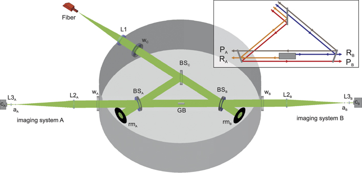
Figure 1. Experimental setup of PTB's DEI. L: lens, w: window of the vacuum-tight chamber, BS: beam splitter, rm: reference mirror, GB: gauge block, a: aperture, c: camera. Detailed description in the text. Inset: pathways of the four measurement beamlines.
Download figure:
Standard image High-resolution imageAn iodine-stabilized Nd:YAG laser (λ = 532 nm) and an additional frequency-stabilized He–Ne laser (λ = 633 nm) are used as light sources and coupled in sequence into the same 200 μm diameter multimode fiber. The current wavelength can be selected by blocking the other laser in front of the fiber coupler. While the small spatial coherence of the multimode fiber reduces unwanted interference, it also generates speckle patterns. To eliminate these patterns, a shaking device is attached to the fiber in a process similar to that described in [21]. Thus, a homogeneous intensity distribution is achieved. If a higher spatial coherence were necessary, also the use of a single mode fiber is possible [15, 16].
The tip of the multimode fiber is used as a point light source. The light emitted is collimated by a lens with a diameter of 100 mm and a focal length of 500 mm. After being transmitted through a window (WC) into the vacuum-tight chamber, the beam is evenly split into the two symmetrical arms (A and B) of the interferometer by a 50/50 beam-splitter plate (BSC). To avoid parasitic interference, all optical plates in the setup have a wedge angle of 10 arcmin, while the back surfaces of the beam splitters are coated with an anti-reflective coating.
Two additional beam splitters (BSA and BSB) divide both beams again into a transmitted reference beam and a reflected object beam. In arm A, the reference beam is reflected at the reference mirror RMA and reflected again at BSA toward the imaging system A. This beam is called RefA in the following. The central part of the object beam is reflected from the gauge block and directed to imaging system A, where it interferes with the RefA beam. The outer part passes the gauge block before reaching imaging system B, where it interferes with reference beam B (RefB). The reflected beam is called RA in the following, whereas the passing beam is called PB. The beams along arm B are described in the same way as those along arm A.
Each imaging system projects a sharp image of the corresponding measuring face of the gauge block onto a CCD camera. Each reference mirror is situated on a three-axis tilt mount, as this allows its tilt to be aligned and its motion to be parallel to that of the incoming beam. This parallel motion makes it possible to evaluate the length differences of the optical beam paths by means of a five-step phase-shift algorithm [22].
The lengths of four different beam paths are used to calculate the measured length LDEI of the gauge block (see inset of figure 1), which is the combination of the beams reflected from the gauge block (RA and RB) and those passing the gauge block (PA and PB). The two additional beam paths via the reference mirrors (RefA and RefB) are used to evaluate each optical path length:


2.1. Alignment of the interferometer
An initial alignment procedure for an earlier prototype [15] was revised during the development of the current interferometer [16]. Further improvements led to the following strategy being devised:
The entire alignment process is carried out with only the 532 nm laser, since the 633 nm laser is mainly used for finding the integral order of interference via the method of exact fractions [23].
First, the fiber must be positioned in such a way that it is within the focal point of the collimation lens (L1). To this end, the lens is placed at a distance of approximately its focal length in front of the fiber tip. The lens is then tilted and the fiber is moved laterally until the back reflections of the lens surfaces overlap in the center of the end of the fiber. This brings the fiber tip approximately into the optical axis of the lens. The lens mount has a removable mirror attached behind the lens perpendicular to its optical axis. The light reflected from this mirror is coupled back into the fiber. To further improve the fiber position, the fiber tip is mounted on an x–y translation stage that automatically scans over a lateral shift of 100 μm in both directions. During this scanning stage, the recoupled intensity is measured at the reverse end of the fiber. The fiber tip is then adjusted in such a way that it is in the center of the measured intensity distribution. The final displacement is less than 10 μm from the optical axis. To align the fiber axially, a shearing interferometer is used in order to create a collimated beam. The axial alignment is experimentally determined to be better than 2 μm.
In the next step, the reference mirrors are aligned to be in autocollimation to the incoming beam. This step is similar to [24] but the reference mirror is tilted instead of the fiber tip being moved. The tilt of each mirror over two different axes is scanned by means of the three piezo pushers of the mirror mount while the light recoupled into the fiber is measured. The optimum tilt coincides with the center of the intensity distribution measured. For the alignment of RMA, an automated shutter between BSC and BSB is closed and only the back reflection of RMA couples into the fiber. Similarly, the tilt of RMB is aligned with the shutter between BSC and BSA being closed. The standard deviation of repeated tilt adjustments is less than 0.7 μrad.
For further alignment of the interferometer, it is necessary to obtain images of the interference pattern on the two cameras. Each imaging system consists of two lenses (L2, L3) with focal lengths f1 = 500 mm and f2 = 40 mm, positioned at a distance of f1 + f2 from each other. A small aperture with a 2 mm diameter is placed at the focal point between the two lenses in order to block unwanted beams that result from multiple reflections in the wedged optical plates. Each camera is adjusted along the optical axis to achieve a sharp image of the corresponding gauge-block surface on its CCD. The sharp image allows the center position of the gauge block in the recorded image to be calculated and the central length to be evaluated. Each imaging system is aligned independently of the rest of the system along an optical bench that can then be aligned as one unit with regard to the interferometer. Since the beam exiting the vacuum-tight chamber is collimated, it is sufficient to align the imaging units via a simple lateral movement and tilting until the focal spot is in the center of the aperture. Via lateral movement, the field of view of the camera can be adjusted until most of the beam, and thus a reasonable image area, has been captured.
To prevent a cosine error (described in section 4.1), the beams traveling in opposite directions between BSA and BSB must be parallel. At the same time, high interference contrast must be achieved. Due to the small spatial coherence length of the light emitted from the multimode fiber, this can be achieved only by precisely overlapping these two beams. A removable crosshair between the collimation lens (L1) and the entrance window (WC) is used to produce a reference point. The lateral shifts between the crosshair images in the passing beams (P) and the reference beams (Ref) can be observed by the two cameras. The beam splitters BSA and BSB are each tilted over two perpendicular axes in such a way that the images of the crosshairs overlap on both cameras. If necessary, the imaging systems can be realigned simultaneously to maintain the desired image area on the cameras. Since transmission through the beam splitters is also altered by tilting them, the autocollimation of the two reference mirrors must be realigned. As the reflections of these mirrors produce the reference crosshairs for aligning the beam splitters, this alignment procedure of beam splitters and reference mirrors must be carried out iteratively until the image of the crosshair is overlapped on both cameras while the reference mirrors are in autocollimation. After this step, the two opposite beams nearly overlap and are nearly parallel. To improve the parallelism, one of the beam splitters can then be very finely aligned until no fringe is visible in the interference image on the cameras. The tilt necessary is so small that the autocollimation is not significantly affected. This results in an angle alignment of the beam splitters that is better than 1.7 μrad, which would correspond to one visible interference fringe on the camera.
Finally, the tilt of the gauge block is aligned until no interference fringe is visible on camera A. Here, if the parallelism of the gauge block is good, no fringe will be visible on camera B, either.
3. Virtual experiment
The virtual experiment of the DEI has been carried out using SimOptDevice, which is a flexible library for virtual experiments developed at PTB. SimOptDevice is implemented in MATLAB® [25] and covers a large range of applications. It supports the development and testing of measurement procedures, and it facilitates the design of experiments. SimOptDevice has also been applied to optimize experiments. Successful applications include the evaluation of the accuracy of interferometric measurements or the development of a deflectometric flatness reference at PTB [26–28].
SimOptDevice allows to define optical and mechanical components in hierarchical coordinate systems and calculating beam paths by ray tracing and ray aiming. Its main advantage over other available software solutions is the fact that it allows users to have full control over all optimization parameters and applied algorithms. Every component and group of components is set into a separate coordinate system (CS) that is adjustable relative to its superior CS. The way in which these CSes are positioned and tilted within a main CS corresponds to the positions in the real interferometer.
In the following, the implementation of the virtual experiment using SimOptDevice is described in detail.
3.1. Alignment of the virtual experiment
The absolute positions of the optical components are not known with enough accuracy to create a perfect virtual copy of the interferometer. However, it is sufficient to study the tilts of the components, since the influence of the absolute positions of flat surfaces is negligible. Therefore, the positions of the components are defined approximately and their tilts are aligned according to the proposed alignment method of the real interferometer. The crucial relative positions between the lenses and their focal points can be calculated via ray tracing. In order to reproduce the real interferometer as accurately as possible, a virtual alignment procedure is implemented that is following the same steps as in the real system.
First, the distance between the point source and the collimating lens (L1) is set to the focal length; the collimated beam travels in a straight line and is aimed at RMA.
Since it is possible to calculate the position and direction of all rays at any point in the interferometer, there is no need to iteratively align the beam splitters and the reference mirrors. To align the tilts of the beam splitters BSA and BSB, a virtual plane is introduced between the collimation lens (L1) and the window (WC) perpendicular to the beam direction. Via ray tracing to this plane, the position as well as the corresponding directions of a number of rays are defined. Each of these rays is then separately traced along the two interferometer arms to a second virtual plane at the position of the gauge block. In order to overlap both beams, each pair of rays must strike this plane at the same position. Additionally, the two opposite rays must be parallel.
The reference mirrors are optimized by fulfilling the criterion that the incidence of all rays to the corresponding mirror must be perpendicular.
The orientation of the lenses in the imaging systems is defined by their optical axes and focal lengths. The tilt of the whole imaging system is optimized in such a way that the incidence of all rays is perpendicular to the camera plane. The system is then laterally moved in such a way that the camera plane is centered on the bundle of incoming rays. This is followed by the axial movement of the virtual camera (relative to L3) toward the sharp image plane of the gauge-block surface. The position of this plane is calculated by tracing rays from a virtual point source in the center of the corresponding gauge-block surface to their focal spot behind the imaging lenses.
Due to the wedge of the windows and beam splitters, the circular beams change their shapes slightly. Hence, the tilts of the previously aligned beam splitters still produce an angle between the beams from the opposite arm and the beam from the reference mirror onto the camera. This is equal to visible fringes in the interference image on the camera. Following the alignment in the real system, BSB is again tilted until the angle between the two beams on camera A is minimal (i.e. corresponds to vanishing interference fringes). To this end, rays from the virtual camera pixels are aimed at the light source along the pathway of the gauge block, passing beam (PA) as well as the pathway via RMA (RefA). The tilt of BSB is varied in such a way that the optical path differences between each pair of rays which start at the same position on the camera plane along the two beam paths are equal. Then, the tilt of RMB and the axial position of camera B are again checked and realigned.
In the last step, the tilt of the gauge block is aligned in the following way. The optical path difference between the rays reflected from the corresponding gauge block surface (RX) and those reflected from reference mirror (RefX) is calculated for a bundle of rays. The gauge block tilt is then varied in such a way that the optical path difference for every pair of rays is equal, which is similar to a camera image without fringes in the real experiment.
Virtual length measurement is performed by 'ray aiming' the defined beams onto the virtual camera pixels. To closely reproduce the real experiment, one can calculate the optical path lengths of all six beams for a whole camera array of 1024 × 1024 pixels. As mentioned earlier, the pathways via the reference mirrors cancel each other out and vanish in the equation for calculating the length (see equation (2)). Therefore, in order to calculate the measured length, it is sufficient to calculate the passing (PX) and reflected (RX) beams from the gauge block. In order to further increase the performance, only the four rays that hit the corresponding gauge-block surface in the center are traced. The beams are aimed at these points to obtain the starting angle at the light source and then traced to the camera. From the four resulting optical pathways, the measured length is calculated in accordance with equation (2).
4. Influences of alignment errors
The virtual experiment is used to individually examine different sources of alignment errors. The main alignment error in the length measurement of gauge blocks is known as the cosine error. In addition to this, there are a number of other effects, some of which occur only in DEIs. The effects are described below and their differences in SEIs and DEIs are shown.
4.1. Cosine error
Due to the increased number of beams in the DEI, the cosine error does not depend exclusively on the misalignment of the gauge block. The parallelism of the two beams from the two interferometer arms that pass the gauge block in opposite directions are also of crucial importance. The measured length in an SEI and a DEI is


where α and β are the angles of the incoming beam to the surface normal of the gauge block on sides A and B respectively.
The angle between the two opposite beams can be substituted by γ = α + β. It is notable that the equation for the DEI is reduced to that for the SEI, not only if the beam splitters are perfectly aligned and γ = 0, but also if α = β. Furthermore, the equation for SEI can be extended if both sides of a gauge block are measured and the length is given as the average of both measurements. This means that the gauge block is measured once with each side wrung to a reference plate, while in each measurement, there is a misalignment of α or β.
4.2. Perpendicularity between measuring faces and side faces
One major difference between length measurements in a DEI compared to measurements in an SEI are the reference points on the gauge block or reference plate. In SEI length measurements, ISO 3650 defines the central length of gauge blocks as the perpendicular distance from the reference plate to the center of the measuring face. For interferometric measurements in practice, this means the center of the free face must be determined to allow the optical path length of its reflected light to be directly measured. The optical path length reflected from the reference plate must be interpolated to the corresponding point which is hidden by the gauge block.
Since, in DEI measurements, the two gauge block end faces are imaged independently, there is no such direct reference between the two end faces. Therefore, it is usually assumed that the gauge block is a perfect cuboid where all faces meet at a right angle and the opposite measuring surfaces are parallel. However, according to ISO 3650, the tolerance of the perpendicularity of a side face with a measuring face of a 100 mm grade K gauge block, for instance, is 100 μm. Therefore, real gauge blocks might have a shape like that in the inset of figure 2.
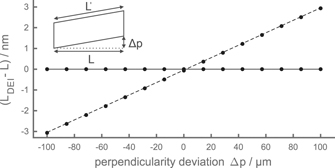
Figure 2. Deviation of the simulated measured length LDEI from the true length L of a rhombic gauge block in dependence on the deviation of perpendicularity Δp between its measuring faces and side faces. Solid line: optimized alignment, dashed line: gauge block tilt of 30 μrad. The dots are simulated data points and the lines are calculated from equation (6).
Download figure:
Standard image High-resolution imageFor a perfectly aligned system there is no difference in the measured length for gauge blocks with different perpendicularities. However, for a slight gauge block tilt the influence of the cosine error increases with decreasing perpendicularity. In figure 2, the measured length deviation in dependence on the perpendicularity deviation of a 100 mm gauge block is shown. The dots represent results of simulated length measurements. As long as the interferometer is optimally aligned and no cosine error occurs the measured length deviation is negligible (solid line). However, if the gauge block is slightly tilted, it is to be seen that the influence of the cosine error increases with a higher deviation from perpendicularity. For a gauge block tilt of ω = 30 μrad, the cosine error can be up to 3 nm, whereas for a perpendicular gauge block it would be less than 0.07 nm. For a wavelength of λ = 532 nm, this tilt corresponds to one visible interference fringe on the cameras along the gauge block's short axis of 9 mm, which is the same magnitude as the alignment accuracy.
Thus, the influence of the cosine error in connection with non-perfect gauge blocks differs from that of perfect gauge blocks. A perpendicularity deviation of Δp is equivalent to an angle deviation ɛ = arctan(Δp/L) from 90°. The distance between the two central points of the end faces is therefore L' = L/cos(ɛ). This can be described as an effective length for the cosine error in equation (4), while the gauge block is tilted by ɛ. The measured length can then be described by


where ω is an additional gauge block tilt due to misalignment. With α = ω and β = −ω, this equation is consistent with equation (4). The result is a shift in the tilt of the gauge block at which the measured length is at its maximum (see figure 3).
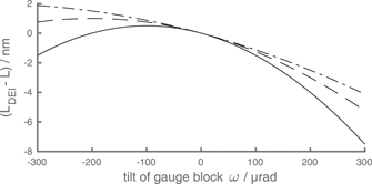
Figure 3. Deviation of the measured length LDEI from the true length L of rhombic gauge blocks with a perpendicularity between its measuring faces and side faces of 10 μm and different lengths in dependence on the tilt ω of the gauge block. Solid line: L = 100 mm, dashed line: L = 50 mm, dash-dotted line: L = 25 mm.
Download figure:
Standard image High-resolution imageFor small tilts of the gauge block, this error is mainly independent of the absolute gauge-block length L. This can be seen in the derivative with respect to the gauge block tilt

which is −y for α = 0.
Besides the alignment error, the deviation from perpendicularity has to be considered while correcting for wavefront aberrations in DEIs. Nonetheless, in the following simulations, all gauge blocks are assumed to be perfectly perpendicular between their measuring faces and their side faces to explicitly distinguish between the error sources. Only in the Monte Carlo runs with non-perfect gauge blocks in section 6 we considered this shape deviation.
4.3. Parallelism of the measuring faces
Another simplification of the gauge block's shape is the parallelism of the two end faces of the gauge block. Although the tolerance is 0.1 μm for grade K gauge blocks that are shorter than 300 mm, the deviation can be dramatic for other measurement standards. Additionally the parallelism of the measuring faces depends on the choice of supporting points while mounting the gauge block. We will assume in this study, that exactly the Airy points are chosen, although in the real experiment this is only an approximation. In SEI length measurements, the measuring method does not change in case of deviations from parallelism of the measuring faces. The reference plate must still be perpendicular to the incoming beam, resulting in a tilted front face of the gauge block. In DEIs, on the other hand, both end faces are observed at the same time and only one face can be tilted in an ideal fashion.
To be close to the definition, the gauge block should be aligned in a completely perpendicular orientation on one side, neglecting the opposite side. However, the uncertainty due to the camera misalignment would be smaller if both sides of the gauge block were misaligned equally (see section 4.4). Similarly to measurements in an SEI it should be stated, which side of the gauge block has been used for the alignment or if the length has been measured in both alignment states. Due to the parallelism of the two opposing beams, a measurement in the DEI with one measuring face aligned perpendicular to the incident beam corresponds to a measurement in an SEI where the same side is wrung to the reference plate.
4.4. Camera defocusing
An incorrectly measured length can be the result not only of a cosine error, but also of an incorrect camera position. First, the image of the gauge block is used to detect the center of the gauge block. To this end, sharp edges in the image are necessary. Second, all beams must have the same optical path distance from the gauge block's measuring surface to the camera, regardless of their direction. The latter concept will be explained in the following.
In figure 4, the path of the beam reflected from the gauge block RB is shown for a tilted gauge block. The two imaging lenses focus a point of the gauge block's surface onto the sharp image plane s. The beam passing the gauge block PB is also imaged onto the plane s. Due to the nature of the imaging system, both beams have the same optical pathway between the gauge block's surface and the plane s. However, if the camera is axially misaligned, the optical pathways of the two rays change differently. Thus, if the camera distance to the imaging lenses is too long, for the change in the optical path length ΔLP,B < ΔLR,B applies, and hence, the measured length is shortened (see equation (2)).

Figure 4. Sketch of the optical beam paths under a tilted gauge block. The beam PB comes from BSA (not shown) and passes the gauge block (GB); the beam RB comes from BSC (not shown) and reflects at BSB onto the gauge block, where it is reflected back. Both beams transmit through BSB and the imaging lenses with principle planes H1 and H2 onto the camera (cam). s is the sharp image plane.
Download figure:
Standard image High-resolution imageFigure 5 shows how a misalignment of one camera can influence the measured length.

Figure 5. Deviation of the simulated measured length LDEI from the true length L in dependence on the axial camera displacement d. The gauge block is tilted by 30 μrad with respect to its perfect alignment, which corresponds to one fringe on the gauge block face along the short axis. The dots are simulated data and the solid line is calculated from equation (8).
Download figure:
Standard image High-resolution imageThe error can be calculated by

where d is the displacement of the camera from the sharp image plane, α is the tilt of the gauge block and f2 and f3 are the focal lengths of the lenses in the imaging system. Since this effect is combined with the cosine error, the measurement of the gauge block can be not only too short (as usually observed), but also too long (see ▽ in figure 6).
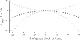
Figure 6. Deviation of the simulated measured length LDEI from the true length L in dependence on the tilt of the gauge block α. The black crosses indicate the optimized axial camera position, and ▽ and △ are results for axial camera displacements of 1 mm to or away from the imaging lenses, respectively.
Download figure:
Standard image High-resolution imageIt is especially important that this defocusing effect be taken into account for DEIs in which both end faces of the gauge block are imaged to a single camera. Several approaches to set up a DEI propose, for example, simply adding a corner cube or a roof mirror to an SEI [7, 10, 12]. In these setups, it is not possible to optimally adjust the focus on both end faces. In SEIs this effect may also occur for non-parallel gauge blocks.
5. Validation of the virtual experiment
The virtual experiment is validated by a comparison to data from a real experiment. For this purpose, the following experiment is applied.
5.1. Validation through measured data
A lateral displacement Δx of the fiber tip tilts the collimated beam entering the interferometer by the angle  . Thus, the two opposite beams at the gauge block are tilted by the same amount ω, but in opposite directions. With β = −α, equation (4) reduces to


In this case, the influence of the camera position is negligible, since the reflected beam at the gauge block (RX) has the same direction of propagation as the beam coming from the other side that passes the gauge block (PX). There is also no relative influence of a rhombic gauge block shape, since the gauge block is not tilted (only the incoming beam is tilted). In figure 7, experimental measured length differences are plotted against the lateral shift of the fiber tip together with simulated data and a fit of equation (10).
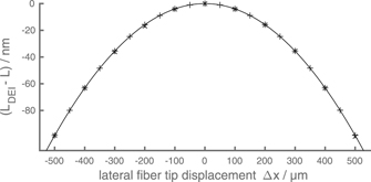
Figure 7. Deviation of the measured length LDEI from the true length L depending on a lateral displacement Δx of the fiber tip from the focal point of the collimating lens. ×: experimental data, +: simulated data, solid line: equation (10).
Download figure:
Standard image High-resolution imageThe tilt of the beams introduced by a lateral fiber displacement can be largely compensated by aligning the beam splitters BSA and BSB. The remaining astigmatism, as well as a spherical wavefront deformation introduced by axial translation, can be compensated by wavefront corrections. Since there are many other contributions to wavefront distortion, the axial position is set to its optimal position and is not investigated further here. For the same reason, the astigmatism introduced is not investigated in this paper further. However, the fiber tip translation allows a comparison between the experimental measurements and the simple theoretical equation, since most other alignment effects are negligible.
5.2. Alignment errors in the real interferometer
Generally, it is not possible to separate the different effects in the real interferometer. To observe alignment errors in the real experiment we used a 200 mm silicon single crystal gauge block which provides high stability over time and is well known from laboratory-internal comparisons carried out in the past. In figure 8 the results for the length measurement of this gauge block in dependence on the gauge block tilt is shown. The measured gauge block has a clear rhombic shape with a distinct deviation from right angles. Therefore, the maximum value of the measured length is not centered on a perpendicular incidence on the measuring surface. The orientation of the gauge block is depicted along the graph. Furthermore, the deviation is not symmetric to the gauge block tilt, indicating the influence of a defocused camera.
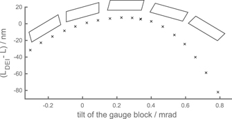
Figure 8. Deviation of the measured length LDEI from the measured length at zero-fringe alignment in dependence on the gauge block tilt ω. The cosine error is distorted due to alignment errors in the beam splitter tilts, the axial camera shifts and the rhombic shape of the gauge block. The pictograms show the orientation of the rhombic gauge block.
Download figure:
Standard image High-resolution imageThe effective length for the cosine error (see equation (6)) can dramatically increase the uncertainty due to a tilted gauge block, since the slope of the cosine becomes larger for perfectly aligned gauge blocks as the angle deviation from 90° increases.
6. Monte Carlo experiment
The virtual experiment is used to quantitatively examine the size of the total uncertainty influenced by alignment errors via a Monte Carlo experiment. The distributions of misalignment in the tilts of the different components were therefore estimated in the following way.
All components in the interferometer are tilted by means of stepper motors or piezo actuators, which generate heat. To reduce the influence of temperature drifts on the measurement, it is important to wait between the alignment and the measurement until temperature equilibrium is achieved in the vacuum-tight chamber. Due to slow mechanical drifts, the alignment status may decrease during this time. This is taken into account in the estimation of the distributions. All alignment values are assumed to be normally distributed. The standard deviations of the distributions are listed in table 1. If a significant part of an interference fringe is visible on one of the gauge block surfaces or in the surrounding area, the beam splitters or the gauge block are realigned before measuring. Therefore, the distributions are truncated at 3σ. All other parameters were not modified. The wavelength has been set to exactly 532 nm and the refractive index in the chamber to n = 1. We thereby obtain the pure uncertainty contribution from the alignment.
Table 1. Considered misalignments in the Monte Carlo runs. All values are assumed to be normally distributed with a standard deviation σ. Some of the distributions are truncated as listed.
| BSA, BSB | Gauge block, fringes along | RMA, RMB | Cameras A, B | ||
|---|---|---|---|---|---|
| Both axes | Short axis (9 mm) | Long axis (35 mm) | Both axes | Axial positions | |
| σ | 1.25 μrad | 11.1 μrad | 28.5 μrad | 0.7 μrad | 0.5 mm |
| Corresponds to | 3/8 fringes | 3/8 fringes | 3/8 fringes | — | — |
| Truncated | 3σ | 3σ | 3σ | — | 3σ |
In general, after the vacuum-tight chamber is evacuated and thermally stabilized, the alignment status is very stable over several days, with less than one fringe visible on the beams passing the gauge block. However, the gauge block usually has to be realigned on a daily basis; occasionally, a small alignment correction of one of the beam splitters is also necessary.
The distribution of the measured length deviation for a perfectly shaped gauge block is shown in figure 9. The shortest 95% coverage interval is ![$\left[-0.09,0.03\right]\enspace \mathrm{n}\mathrm{m}$](https://content.cld.iop.org/journals/0026-1394/58/6/064001/revision3/metac2724ieqn2.gif) . The alignment precision of the DEI is therefore sufficient for length measurements in the sub nanometer scale.
. The alignment precision of the DEI is therefore sufficient for length measurements in the sub nanometer scale.
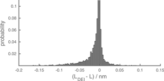
Figure 9. Distribution of the measurement deviation from the true length (LDEI − L) in a Monte Carlo experiment. Detailed description in the text.
Download figure:
Standard image High-resolution imageHowever, for real gauge blocks with non-perfect perpendicularity between the measuring faces and side faces or parallelism of the measuring faces, the uncertainty of the measured length is larger. Distributions of the measured length deviation of different gauge block shapes are shown in figure 10. The considered form deviations of the gauge block are listed in table 2. The simulated gauge-block length is 100 mm and the deviation from parallelism is 0.07 μm, except for the dotted line where the length is 25 mm and the end faces are perfectly parallel. The deviation from perpendicularity was varied between the simulations. For the solid line, it was 100 μm, for the black dashed/dotted line, it was 50 μm, for the gray dashed/dotted line, it was 25 μm and for the dashed line as well as the dotted line, it was 10 μm.

Figure 10. Distribution of the measurement deviation from the true length (LDEI − L) in a Monte Carlo experiment for different non-perfect gauge blocks. Detailed description in the text.
Download figure:
Standard image High-resolution image
Table 2. Length and form deviations of the simulated gauge blocks. Different deviations from perpendicularity between the measuring faces and the side faces as well as from the parallelism of the two measuring faces were considered.
| Length | Perpendicularity | Parallelism | Coverage interval | |
|---|---|---|---|---|
| L/mm | Δp/μm | 1/μm | 1/nm | |
| Perfect gauge block | 100 | 0 | 0 |
![$\left[-0.09,0.03\right]$](https://content.cld.iop.org/journals/0026-1394/58/6/064001/revision3/metac2724ieqn3.gif)
|
| Solid line (limits of grade K) | 100 | 100 | 0.07 |
![$\left[-0.66,0.63\right]$](https://content.cld.iop.org/journals/0026-1394/58/6/064001/revision3/metac2724ieqn4.gif)
|
| Black dashed/dotted | 100 | 50 | 0.07 |
![$\left[-0.34,0.32\right]$](https://content.cld.iop.org/journals/0026-1394/58/6/064001/revision3/metac2724ieqn5.gif)
|
| Gray dashed/dotted | 100 | 25 | 0.07 |
![$\left[-0.19,0.16\right]$](https://content.cld.iop.org/journals/0026-1394/58/6/064001/revision3/metac2724ieqn6.gif)
|
| Dashed | 100 | 10 | 0.07 |
![$\left[-0.11,0.07\right]$](https://content.cld.iop.org/journals/0026-1394/58/6/064001/revision3/metac2724ieqn7.gif)
|
| Dotted | 25 | 10 | 0 |
![$\left[-0.09,0.08\right]$](https://content.cld.iop.org/journals/0026-1394/58/6/064001/revision3/metac2724ieqn8.gif)
|
The deviations for the solid line correspond to the limits of a grade K gauge block with a length of 100 mm. The shortest 95% coverage interval is ![$\left[-0.66,0.64\right]\enspace \mathrm{n}\mathrm{m}$](https://content.cld.iop.org/journals/0026-1394/58/6/064001/revision3/metac2724ieqn9.gif) (i.e. more than ten times larger than for perfect gauge blocks).
(i.e. more than ten times larger than for perfect gauge blocks).
The main influence is traceable to the deviation from perpendicularity between the measuring faces and side faces. As described in section 4.2, this leads to a significantly higher contribution of the cosine error. Comparing the dashed line and the dotted line reveals that the absolute length and the deviation from parallelism is negligible considering only the alignment. For example, the contribution of not probing the precise center must also be considered. However, since this is not a contribution due to the alignment or the fundamental choice of the reference points, we will neglect this here. For the dashed line, the shortest 95% coverage interval is ![$\left[-0.11,0.07\right]\enspace \mathrm{n}\mathrm{m}$](https://content.cld.iop.org/journals/0026-1394/58/6/064001/revision3/metac2724ieqn10.gif) while for the dotted line, it is
while for the dotted line, it is ![$\left[-0.09,0.08\right]\enspace \mathrm{n}\mathrm{m}$](https://content.cld.iop.org/journals/0026-1394/58/6/064001/revision3/metac2724ieqn11.gif) . A perpendicularity of better than 10 μm would therefore be needed to minimize the measured uncertainty.
. A perpendicularity of better than 10 μm would therefore be needed to minimize the measured uncertainty.
7. Conclusion
The alignment process for PTB's DEI, for contactless length measurements of gauge blocks has been described. The different sources of alignment errors have been discussed and differences to single-ended interferometry are revealed. Theoretical relations have been verified by virtual experiments and the impact of these relations on experimental data has been demonstrated. Particularly the effects of camera defocusing and real gauge blocks which deviate from the ideal cubic geometry are described.
The central point of each measuring face is used for measuring the central length of a gauge block. Due to the lack of a direct reference between the two imaged faces this is a reasonable approach for prismatic bodies with small shape variation from a cubic. Although, this does not correspond exactly to the definition of the length of a gauge block. In order to lower the contribution of non-perfect gauge-block shapes, the perpendicularity of adjacent faces has been found to be essential.
Furthermore, Monte Carlo runs of the virtual experiment have shown that the deviation of the measured length due to alignment errors and mechanical drifts lies in a 95% coverage interval of ![$\left[-0.66,0.63\right]\enspace \mathrm{n}\mathrm{m}$](https://content.cld.iop.org/journals/0026-1394/58/6/064001/revision3/metac2724ieqn12.gif) for grade K gauge blocks down to theoretical
for grade K gauge blocks down to theoretical ![$\left[-0.09,0.03\right]\enspace \mathrm{n}\mathrm{m}$](https://content.cld.iop.org/journals/0026-1394/58/6/064001/revision3/metac2724ieqn13.gif) for gauge blocks without form deviations. Hence, it has been confirmed that the given alignment process is highly accurate for performing length measurements. For the actual length measurement of high quality gauge blocks, the goal has been achieved to show that the uncertainty due to the alignment is therefore of minor significance compared to other influences, such as temperature deviations, wavefront aberrations and surface properties of the measuring face.
for gauge blocks without form deviations. Hence, it has been confirmed that the given alignment process is highly accurate for performing length measurements. For the actual length measurement of high quality gauge blocks, the goal has been achieved to show that the uncertainty due to the alignment is therefore of minor significance compared to other influences, such as temperature deviations, wavefront aberrations and surface properties of the measuring face.