

Abstract
Observing and timing a group of millisecond pulsars with high rotational stability enables the direct detection of gravitational waves (GWs). The GW signals can be identified from the spatial correlations encoded in the times-of-arrival of widely spaced pulsar-pairs. The Chinese Pulsar Timing Array (CPTA) is a collaboration aiming at the direct GW detection with observations carried out using Chinese radio telescopes. This short article serves as a "table of contents" for a forthcoming series of papers related to the CPTA Data Release 1 (CPTA DR1) which uses observations from the Five-hundred-meter Aperture Spherical radio Telescope. Here, after summarizing the time span and accuracy of CPTA DR1, we report the key results of our statistical inference finding a correlated signal with amplitude  for spectral index in the range of α ∈ [ − 1.8, 1.5] assuming a GW background (GWB) induced quadrupolar correlation. The search for the Hellings–Downs (HD) correlation curve is also presented, where some evidence for the HD correlation has been found that a 4.6σ statistical significance is achieved using the discrete frequency method around the frequency of 14 nHz. We expect that the future International Pulsar Timing Array data analysis and the next CPTA data release will be more sensitive to the nHz GWB, which could verify the current results.
Export citation and abstract BibTeX RIS
Corrections were made to this article on 5 July 2023. Corrections were made to the acknowledgments section.
1. Introduction
A Pulsar Timing Array (PTA; Foster & Backer 1990) is an array of pulsars, which are regularly observed. The times-of-arrival (TOAs) are measured for pulses that we see beams of electromagnetic waves emitted by the pulsars sweeping over the Earth. As the directions of the radiation beam and the pulsar rotational axis do not coincide, we observe this radiation as regular pulses synchronized to the pulsar rotation (Gold 1969). By extracting correlated signatures in pulsar TOAs, it is possible to detect GWs (Hellings & Downs 1983; Jenet et al. 2005), measure masses (Champion et al. 2010; Caballero et al. 2018) and orbital elements of solar system planets (Guo et al. 2019), and study the stability of international (Hobbs et al. 2012, 2020) and local (Li et al. 2020) atomic time standards.
At present, the PTA experiment is the only known effective method to detect gravitational waves (GWs) in the nanohertz (nHz) band. It was predicted that the orbiting and merger of supermassive black hole binaries (SMBHBs) would create a stochastic nHz GW background (Sesana 2013), while alternative channels, including cosmic strings (Kibble 1976; Sanidas et al. 2012) and relic GWs from early universe processes (Grishchuk 2005; Zhao et al. 2013; Lasky et al. 2016), are also possible. All these sources provide the GWB targets for PTA experiments. While in addition, PTAs are also able to detect GWs from single SMBHB systems (e.g., Jenet et al. 2004; Sesana et al. 2009; Lee et al. 2011). At present, six major regional PTAs exist: Parkes Pulsar Timing Array (PPTA, Manchester 2008; Manchester et al. 2013; Goncharov et al. 2022), European Pulsar Timing Array (EPTA, Kramer & Champion 2013; Chalumeau et al. 2022), North American Nanohertz Observatory for Gravitational Waves (NANOGrav, Jenet et al. 2009; Arzoumanian et al. 2020), Indian Pulsar Timing Array (InPTA, Nobleson et al. 2022), South Africa Pulsar Timing Array (SAPTA, Spiewak et al. 2022), and Chinese Pulsar Timing Array (Lee 2016). The International Pulsar Timing Array (IPTA, Manchester & IPTA 2013) is a consortium of the regional PTA consortia aiming at a better GW sensitivity. Currently, the PPTA, EPTA, NANOGrav, and InPTA are formal IPTA members, while SAPTA and CPTA are IPTA observers.
Here, we report the progress of CPTA efforts. The current status of CPTA observations and data quality are summarized in Section 2. Our statistical inference for the amplitude and spectral index of a nHz stochastic GWB are presented in Section 3. Section 4 includes the search for the GW-induced quadrupolar correlation (i.e., the HD curve). Discussion and conclusions are in Section 5.
2. Observations and Data
The CPTA DR1 consists of TOA measurements and pulsar timing models for 57 MSPs (Xu et al. 2023, in preparation). The data covers the time span between 2019 April and 2022 September. Observations were conducted using the Five-hundred-meter Aperture Spherical radio Telescope (FAST; Jiang et al. 2019), in Guizhou province, China. For most MSPs, the majority of the observations were taken with a cadence of approximately two weeks. Pulsars with smaller timing errors, e.g., PSR J1713 + 0747, were observed more frequently since 2020 February under a CPTA extension proposal. We excluded data of PSR J1713 + 0747 after MJD = 59 319 in our analysis because of the abrupt profile change event (Lam 2021; Singha et al. 2021; Xu et al. 2021; Jennings et al. 2022). The observations were carried out with the central beam of the 19 beam receiver (Jiang et al. 2020) within the frequency range from 1.0 to 1.5 GHz.
Search mode data were recorded with a ROACH 2-based system. 15 The data were folded offline in 30 s intervals using the software package DSPSR (van Straten & Bailes 2011). With the software package PSRCHIVE (Hotan et al. 2004), the data were cleaned by removing radio interference, polarization calibrated (Jiang et al. 2023, in preparation), and integrated over frequency and time. The final number of frequency channels was 64 (∼7.8 MHz resolution), except for PSRs J0218+4232 and J0636+5129, which have many observations, where the number of frequency channels was 16 in order to reduce the size of the data set. The final integration time for integrated pulse profiles was typically 20 minutes, or shorter than 2.5% of the binary period. Our TOAs were generated by cross-matching observed pulse profiles with the standard total-intensity templates. Sub-integrations with low signal-to-noise ratio (S/N < 8) were removed (less than 5.2% in total). More details on the data set can be found in Xu et al. (2023, in preparation).
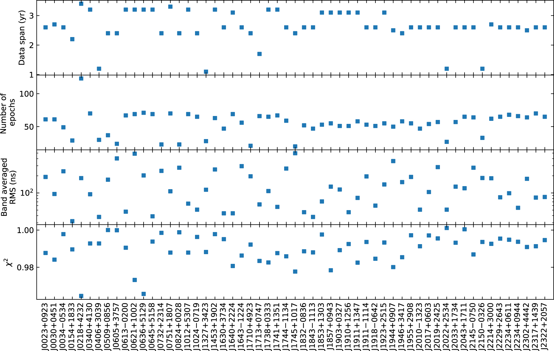
The pulsar timing models were created using the software package TEMPO2 (Hobbs et al. 2006). Our noise model for a single pulsar consists of three components: white, red, and dispersion measure (DM) noise. The white noise is characterized using EFAC, EQUAD, and ECORR parameters. EFAC re-scales the TOA measurements error to account for inaccuracies in the process of TOA extraction using the template-matching method (Taylor 1992), EQUAD adds white noise in quadrature (van Haasteren et al. 2011), and ECORR (NANOGrav Collaboration et al. 2015) models the correlated white noise (phase jitter) among different frequencies in the same epoch (Wang et al. 2023, in preparation). Both red and DM noises are modeled as stochastic stationary processes, assuming power-law spectra, characterized by amplitude and spectral index. Our inference of pulsar noise model parameters is conducted within a Bayesian framework. The definitions of model parameters are well described in the literature (e.g., Lee et al. 2014; Lentati et al. 2014), of which the conventions are followed in our analysis. Four independent noise analysis software pipelines were used, namely, TEMPONEST(Lentati et al. 2014), ENTERPRISE, 16 FORTYTWO(Caballero et al. 2016) and 42++. 17 Consistent results were produced by the four pipelines (Chen et al. 2023, in preparation). We further compared all 16 possible combinations of noise modeling, which use/do not use EQUAD, ECORR, red noise, and DM noise. To avoid overfitting, the final best model is picked by comparing the Bayesian evidence of all 16 models. The data quality of the CPTA DR1 is summarized in Figure 1. The detailed evaluation of how the noise modeling affects the GWB inference will be published by Chen et al. (2023, in preparation).

Figure 1. Summary of the CPTA DR1 data quality. From top to bottom, the panels show data span, number of epochs, weighted root-mean-square (rms) of frequency integrated residuals, and reduced χ2 of timing residual, respectively.
Download figure:
Standard image High-resolution image3. Parameter Inference for the Stochastic GWB
We used the standard frequency-domain Bayesian method (Lentati et al. 2014; van Haasteren & Vallisneri 2014) to perform statistical inference for the amplitude and spectral index of the stochastic GWB. We adopted the following definitions for the amplitude and spectral index of the GWB. The characteristic strain, A(f), of GWB is

where Ac is the characteristic amplitude at the frequency of yr−1, α is the spectral index for characteristic amplitude. For a stochastic GWB induced by the GW-driven merger of SMBHB population, α = − 2/3 is expected when the number of GW sources in the frequency band is sufficiently larger than unity (Phinney 2001). The corresponding single-sided spectral density, S(f), for the GW-induced pulsar timing residuals, i.e., differences between observed TOAs and the model predictions, is (Jenet et al. 2005)

With above definitions, the root-mean-square deviation (rms) σ of the GW-induced pulsar timing residuals is found by applying the Wiener-Khinchin theorem, as

where flow and fhigh are the low and high boundaries defining the frequency band of the GW signal.
We have used the parallel tempering Markov chain Monte Carlo (first applied in the PTA community by Ellis 2013) to perform the posterior sampling, where ten temperatures in a geometric series are used to speed up the initial burning runs and help to find the global maximum of the likelihood function (see the arguments of Neal 1996 and Vousden et al. 2016). The priors of the GWB parameters are uniform ![$\mathrm{log}{A}_{{\rm{c}}}\in [-18,-13]$](https://content.cld.iop.org/journals/1674-4527/23/7/075024/revision5/raaacdfa5ieqn2.gif) and α ∈ [ − 1.8, 1.5]. The prior range of α is determined by the requirement that the rms of the stochastic power-law noise does not diverge after fitting the pulsar period and period derivative (Lee et al. 2012); the lower boundary of −1.8 is set slightly higher than the theoretical requirement, i.e., α > -2.0, to avoid numerical singularities.
and α ∈ [ − 1.8, 1.5]. The prior range of α is determined by the requirement that the rms of the stochastic power-law noise does not diverge after fitting the pulsar period and period derivative (Lee et al. 2012); the lower boundary of −1.8 is set slightly higher than the theoretical requirement, i.e., α > -2.0, to avoid numerical singularities.
Our posterior distribution for the GWB parameters after marginalizing the pulsar timing and noise model is shown in Figure 2, where we marginalized both pulsar timing parameters and noise parameters. Note that we have marginalized over all possible noise parameters without fixing any of them, i.e., our free parameters included white noise parameters, i.e., EFAC, EQUAD, and ECORR, as well as the red and DM noise amplitudes and spectral indices. Using the maximum likelihood estimator for the stochastic GWB amplitude, we recover  (for 95% confidence level), while, because of the limited data span of only about 3 yr, the spectral index α is not well constrained given our prior range of −1.8–1.5. Even so, the distribution of α indicates that the signal is stronger at lower frequencies. If we fix the spectral index to be α = − 2/3 as predicted by the model of GW-driven merger of SMBHBs, the GWB amplitude is
  (for 95% confidence level) and the posterior is shown in Figure 3.

Figure 2. The parameter inference for the stochastic GWB using CPTA DR1. Upper-left: histogram for the posterior distribution of spectral index α. Upper-right: 2D distribution for the spectral index α and GW characteristic amplitude Ac. Bottom-right: histogram for the distribution of GW characteristic amplitude.
Download figure:
Standard image High-resolution image
Figure 3. The histogram for the posterior distribution for the GWB amplitude after fixing the spectral index at α = -2/3.
Download figure:
Standard image High-resolution image4. Searching for the Hellings–Downs Curve
PTAs search for the HD correlation signature (Hellings & Downs 1983) to verify that the correlations in pulsar timing residuals are quadrupolar and induced by an isotropic stochastic GWB. We have searched for the HD correlation in the CPTA DR1. As explained in the previous section, the spectral index of the signal was not well constrained, because of the limited data span. Therefore, instead of searching for the spatial correlation in the framework of power-law spectral models, we performed a more robust search for the spatial correlation at discrete frequencies, such that (1) the results do not depend on the priors of how the correlation function is parameterized and (2) the results do not depend on the spectral shape information. We searched mainly at f1.5 = 14.0 nHz, which corresponds to 1.5/T with T = 3.40 yr being the total time span of the CPTA DR1. The reasons for choosing such a frequency are explained in Appendix B. To check the consistency of results, we also searched at the other two frequencies, i.e., f1 = 9.34 and f2 = 18.7 nHz, respectively. These frequencies correspond to 1/T and 2/T.
A two-step method was used to measure the pulsar-pair correlation coefficients for each discrete frequency. We simultaneously fitted all pulsar timing residuals with the individual pulsar timing models and a common sinusoidal waveform at a given frequency f. After marginalizing the pulsar timing models, the phases of sinusoidal waveforms for each pulsar and the common amplitude were measured using the maximum likelihood estimator as

where  is
is

Here, the subscript i denotes the index of pulsar. Vector
r
i
and matrix
D
i
are the timing residual and timing model design matrix for the ith pulsar, respectively.
λ
T,i
are pulsar timing and noise parameters, e.g., pulsar period, period derivative, white, red and DM noise. C is the pulsar noise covariance matrix. ϕi
is the phase of the correlated signal for the ith pulsar. A is the amplitude of the correlated signal in timing residual, e.g., a GWB-induced signal. Here, amplitude A is proportional to the rms defined in Equation (3) over a narrow frequency band around frequency f. However, due to the irregular sampling of pulsar timing data, there is no close formula to express A in terms of spectral density S(f). One can show that this approach is equivalent to the frequency-domain modeling of power-law processes (van Haasteren & Vallisneri 2014) with one frequency element. The pairwise correlation coefficient between the ith and the jth pulsars is  .
.
The statistical significance for the HD correlation against constant correlation is evaluated using the frequentist method described by Jenet et al. (2005), as

with the average operator over pulsar pairs defined as  , where N is the number of pulsars, ∑i<j
sums over all independent pulsar pairs, and Hij
(for i ≠ j) is the HD function of pulsar pairs that
, where N is the number of pulsars, ∑i<j
sums over all independent pulsar pairs, and Hij
(for i ≠ j) is the HD function of pulsar pairs that

where θij
is the angular distance between the ith and the jth pulsars. The exact expression for the null-hypothesis distribution of  is rather lengthy (Kenney & Keeping 1939). For our case, where the number of pulsars is significantly larger than unity, a much simpler asymptotic Gaussian form is available as explained by Jenet et al. (2005), i.e., the probability density distribution function of
  with no correlation is

It should be noted that this method is immune to the contamination of common uncorrelated signals (Lentati et al. 2015; Arzoumanian et al. 2020; Chen et al. 2021; Goncharov et al. 2021; Antoniadis et al. 2022), because it evaluates the statistical significance only using the cross correlation. Furthermore, the monopolar correlation induced by clock errors is also automatically removed, because the average value of the correlation coefficients is subtracted in Equation (6). Another interesting property of the above statistic is that the error in cij
is regularized such that −1 ≤ cij
≤ 1. On the one hand, this makes the  not the optimal statistic to search for the HD curve. On the other hand, the error of cij
becomes weakly dependent on the pulsar intrinsic noise, and
not the optimal statistic to search for the HD curve. On the other hand, the error of cij
becomes weakly dependent on the pulsar intrinsic noise, and  is less affected by the systematics of a few pulsars with dominant precision. We demonstrate the application of this method with two simulated data sets, where one contains the GWB signal injection (positive control group) and the other does not (negative control group). The simulated data sets are the "clones" of the CPTA DR1 that they have the same frequency resolution and sampling epochs as the CPTA DR1.
The measured pair-wise correlation coefficients of CPTA DR1 are shown in Figure 4, where the results of the negative and positive control groups using simulated datesets are also shown. For the simulated data set without the GWB injection (i.e., the negative control), we detect no significant spatial correlations as shown in the top panels of Figure 4.

Figure 4. The measured correlation coefficients (y-axis) as a function of the pulsar-pair separation angle (x-axis). Red dots denote the measured correlation coefficients between all pulsar-pairs without the auto-correlation. The blue curves with error bars represent the binned average red dots, which only serve to aid the visual inspection. The error bars are the standard error of binned average value estimated using the binned red dots. The solid red curves depict the theoretical HD curve. The top row three panels show simulations without the GWB signal injection, where the data was simulated to match exactly the times and frequencies of the real CPTA DR1. Each panel from left to right corresponds to f = 1/T, 1.5/T, and 2/T, respectively.
Download figure:
Standard image High-resolution imageWe can detect the HD correlation in the positive control with the injected GW signal as shown in the middle panels of Figure 4. In the data set, the characteristic amplitude and spectral index of GWB are Ac = 10−14 and α = − 2/3, respectively. The statistical significance ( ) peaks at f = 1.5/T, whereas it is low at f1 and f2 (
 and
and  , respectively). Such behavior agrees with the theoretical expectation, as explained in Appendix B, that (1) the statistic significance of f = 1/T is lower than that at f = 1.5/T, because fitting of the pulsar timing model affects the low-frequency components of the signal; and (2) the statistic significance at f = 2/T is lower than that at f = 1.5/T, because the power-law spectral signal is weaker at higher frequency.
The statistical significance of the HD correlation of CPTA DR1 shows similar features to those of the positive control group. For CPTA DR1, as shown in the bottom panels of Figure 4,  peaks at 1.5/T, which corresponds to a P-value of PV = 4 × 10⁻⁶. As we saw in the positive control group,
  and 2.3 are lower at f = 1/T and 2/T, respectively. By comparing the positive control group results and the CPTA DR1 results, we can further confirm that the GWB amplitude should be lower than 10−14. We also performed the phase shift and sky position scrambling experiments, which are described in Appendix C.
The signal components of the three frequencies 1/T, 1.5/T, and 2/T are not independent of one another, because the sampling of the data is irregular. It is thus invalid to directly add (in the sense of the square-root sum of squares) the statistical significance at the three frequencies to compute the frequency-integrated statistical significance, even though the frequency-integrated statistical significance is always higher or equal to the statistical significance measured at a single discrete frequency. In the case where noise modeling is not accurate enough, the frequency-integrated statistical significance could be lower than the single frequency value because of statistical fluctuations or wrong weights at some frequencies. This could happen if longer data is used and the signal spectrum over a wide frequency range can not be well described by a single power law.
For the CPTA DR1, we can not discriminate between dipole (cosine function) and HD correlation with only cross-correlation coefficients, although it seems to be lack of physical mechanism to produce the dipole correlation at the frequency we are currently sensitive to. For dipole correlation, we get  at f = 1.5/T, which is only slightly lower than that of HD correlation. If we use the Bayes factor as the statistic (see the method described in Arzoumanian et al. 2020), HD correlation is preferred with a "strong evidence" that the Bayes factor
  . We should point out that one of the major differences between the Bayesian method and the above frequentist method is that the Bayesian method includes the autocorrelation terms in comparing the two models, while the above method does not. Furthermore, Bayes factor
  here is not the perfect touchstone to exclude the dipole correlation interpretation, as demonstrated by numerical simulations of Zic et al. (2022) and the toy model in Appendix A. One needs to be cautious about the application and interpretation of the Bayes factors for the current problem of measuring or detecting the statistical variance of stochastic signals with spatial correlations.
5. Discussion and Conclusion
In this paper, we show that the inferred GWB characteristic amplitude is  for a spectral index in the range α ∈ [ − 1.8, 1.5], and
  if fixing α = − 2/3. The measured GWB amplitude agrees with theoretical expectation (Sesana 2013; McWilliams et al. 2014). However, because of the short span of the CPTA DR1, we cannot yet differentiate between different models of SMBHB formation and evolution. Our GWB amplitude seems to be compatible with that of the common red signal of other PTAs (Arzoumanian et al. 2020; Chen et al. 2021; Goncharov et al. 2021; Antoniadis et al. 2022), although the median of posterior distribution seems to be 0.4–0.5 dex higher. It is possible that a single power law with α = − 2/3 is insufficient to extend the previous results to the high frequency band that CPTA is currently sensitive to, i.e., the spectrum of the GWB signal is not fully power-law in shape and may have a spectral "bump" in the CPTA frequency band (≥10−8 Hz). The statistical significance of the HD correlation over a constant-value correlation in CPTA DR1 is 4.6σ around 14 nHz, i.e., a P-value of 4 × 10⁻⁶. Our correlation-curve analysis is compatible with the GWB amplitude inference, where the comparison between the statistical significance of simulations and CPTA DR1 suggests that the amplitude of GWB quadruple signal A < 10−14. More details, including comparisons between different data reduction pipelines and a cross-check of the current measurements, will be published in a following paper (Xu et al. 2023, in preparation).
For the spatial correlation inference, we measured the pulsar pairwise correlation at single frequencies, which removes the power-law presumption for the GWB spectral shape. Additionally, this method is not affected by common uncorrelated noise or clock error, as it uses only the cross correlations and subtracts their average value. However, this method limits our statistical significance, because only the correlation at a single frequency was extracted. The total statistical significance will be higher than the single frequency values. However, to combine the measurements at multiple frequencies to deliver the frequency-integrated spatial correlation, we would need accurate information on the GWB spectral shape and pulsar noise properties. In the future, we expect that data with a longer span will enable us to go lower in frequency and therefore measure the spectral index with better accuracy.
The current method cannot rule out a dipole origin for the correlation, since both dipole and HD correlations produce similar values of  . If we use Bayesian method to compare the models of dipole and HD correlation, the Bayes factor (with the caveats discussed in Appendix A) prefers the HD correlation that the Bayes factor of HD correlation over dipole correlation is
  .
.
The current CPTA DR1 statistical significance is still below the IPTA "detection" bar of  . Independent results of other regional PTAs may soon help to confirm the current findings. On a longer timescale, we look forward to officially joining the IPTA. By combining IPTA and CPTA data, we expect a further increase in GWB detection sensitivity. The CPTA DR2, scheduled for 2026, is also expected to deliver better accuracy in GWB parameter inference. We are clearly in the era of opening the nHz GW observation window.
Acknowledgments
Observation of CPTA is supported by the FAST Key project. FAST is a Chinese national mega-science facility, operated by National Astronomical Observatories, Chinese Academy of Sciences. This work is supported by the National SKA Program of China (2020SKA0120100), the National Natural Science Foundation of China (Nos. 12041303 and 12250410246), the CAS-MPG LEGACY project, and funding from the Max-Planck Partner Group. K.J.L. acknowledges support from the XPLORER PRIZE and 20 yr long-term support from Dr. Guojun Qiao. The data analysis are performed with computer clusters DIRAC and C*-system of PSR@pku and computational resource provide by the PARATERA company. Software package 42++ is developed with Intel oneAPI toolkits and the Science Explorer's Developing GEars from Weichuan technology. We thank Dr. Jin Chang for providing the valuable long-term support to the CPTA collaboration. CPTA thanks Dr Duncan Lorimer and Dr Michael Kramer for helping initiate the collaboration.
H.X., S.Y.C., Y.J.G., J.J.C., B.J.W., J.W.X., Z.H.X., R.N.C., J.P.Y., Y.H.X., J.B.W. and K.J.L. are core team to perform the data analysis for the current paper, where H.X. worked on data reduction, timing and data analysis; H.X., S.Y.C., Y.J.G. and K.J.L. performed the noise and GWB data analysis; B.J.W. and J.P.Y. carried out single pulse studies; J.J.C. and J.W.X. calibrated data polarization; Z.H.X. and R.N.C. searched for GW single sources; Y.H.X. studied scintillation processes; and JBW studies the GW memory effects. Before FAST observation, LFH and JTL helped test pulsar timing observation with Luonan and Kunming 40 m radio telescopes. K.J.L. organized the team and drafted the current paper. In alphabet order, J.L.H., P.J., Z.Q.S., M.W., N.W., and R.X.X. are the CPTA executive committee members. X.P.W. and R.M. served as the supervise committee members oversee the CPTA collaboration. R.M. helped create the pulsar community in China and the formation of the CPTA. Q.L., X.G., M.L.H., C.S., and Y.Z. are the core FAST support team members.
Appendix A: Is the Bayes Factor Invalid?—Analytic Study of a Toy Model
Here we provide a toy model to illustrate the problems of applying the Bayes factor in the context of common signals. Our toy model contains N pulsars. The timing residuals of all pulsars are just pure white noise. There is neither spatially correlated nor common uncorrelated signal components. The null and positive hypotheses are

We further simplify the toy model by setting the average value of timing residual to be 0. For H0, the parameters of the noise model contain the standard deviation of the timing residual, which is denoted as σi for the ith pulsar. The likelihood of H0 is

The expected value of Bayes evidence (BE) with logarithmic prior (the most common choice in PTA problems) is

For H1, an extra amplitude parameter (A) is required to model the amplitude of the common uncorrelated signal, so that the likelihood function is

Clearly, the expectation of Bayes evidence of H1, i.e.

will not converge on the boundary of ∂∣σi = 0, as the amplitude A modifies the behavior of the exponential function when σi → 0 and the singularity rises because of the logarithmic prior. In other words, the Bayes factor BE1/BE0 can be arbitrarily large no matter what the data is, if one varies the prior range in the current toy model. This is true even the prior range is kept to be the same for both H0 and H1! It is not hard to see that the similar argument is also applicable to the case of comparing two spatially correlated signals, where one will be evaluating the Bayes factor between two singular distributions. Numerical simulations have shown similar features, we refer interested readers to the work of Zic et al. (2022).
Furthermore, although one can regularize the prior singularity by using finite priors, the Bayes factor then becomes prior dependent. Other singular behaviors will rise, when the spatial correlations and spectral properties of signals are considered. All those effects indicate that we should be cautious about applying and interpreting the Bayes factors in the PTA GWB searching problems. To fully utilize the power of Bayes factors, we need (1) the probability distribution function of Bayes factors under the null hypothesis, which requires that the sample space is measurable such that probability distribution function can be well defined, and (2) the computational method to calculate the null-hypothesis distribution of Bayes factors that converges to the full-sample-space expectation at the large N limit.
Appendix B.: Systematic Error of Correlation Coefficients Due to the Fitting of Pulsar Period and Period Derivative
For two cosine functions with the same frequency, i.e.,  and
and  , the correlation coefficient is
  . Here one can regard the two cosine functions as the single-frequency components of GW-induced signals for two different pulsars. In the pulsar timing procedure, one fits for the pulsar period and period derivative. Thus, the best-fitted quadratic is subtracted by-default from the timing residuals. Such a fitting modifies the correlation coefficient between the two cosine functions and leads to a systematic error.
After subtracting the best-fitted quadratic, the two functions are  and
and  , where the coefficients of the quadratic, i.e., α0..2 and β0..2, are found by minimizing the χ2, i.e.


To evaluate the effects of the above quadratic fitting on the correlation coefficient c, we define the rms level of systematic error over all possible correlations as
The systematic error as a function of the frequency f is shown in Figure B1. As expected, it shows that the correlation coefficients of lower frequency components (f ≤ 1/T) are mostly affected. In the paper, we choose f = 1.5/T, such that the systematic error of the correlation coefficient is less than 10%. For future data sets, the frequency can be chosen with a higher value to further reduce the systematic error, as the data sensitivity improves.

Figure B1. The systematic error of correlation coefficients cij due to the quadratic fitting. Here, x-axis is the frequency in the unit of 1/T, and y-axis is the systematic error of correlation coefficients defined in Equation (B3). The vertical dashed line indicates f = 1.5/T.
Download figure:
Standard image High-resolution imageAppendix C: Phase Shift and Sky-position Scramble Experiments
As is common in PTA data analysis at the time this paper is written, we perform the experiments with the phase shift and the sky-position scramble, which were first introduced by Taylor et al. (2017). The recipes for the two experiments are as follows: (i) For the phase shift experiment, one introduces random phase either to the data or Fourier design matrix, which eliminates the phase coherence between pulsars. With each phase shift, the desired statistics in a given GW detection pipeline are computed and collected. The distribution of the collected values of the statistics is then used to form an approximation to the null-hypothesis statistical distribution function to evaluate the false alarm probability. (ii) The sky-position scramble is similar, where one replaces the phase shifting with the scrambled pulsar position, i.e., assigns random positions to the pulsars. The method aims at shuffling the pulsar position to remove the spatial correlation, where one randomly re-assigns all pulsars with new pulsar positions over the entire sky and ensures that the "matching" (see definition in Taylor et al. 2017) is below a prescribed threshold (M) between the scrambled spatial correlation functions. Note, it is required that the matching between any two full skies of the position-scrambles is also below the threshold.
For our statistics  defined in Equation (6), the results of phase shifting and sky position scrambling experiments are shown in Figure C1. One can see that the phase shifting reproduced the expected null hypothesis distribution. This is not surprising. For our statistics, as
  does not depend on the amplitude of the correlated signal, the distribution of
  becomes the null-hypothesis distribution after the correlation between any pulsar pair is destroyed by the random phase shifts. One can get different conclusions, if an alternative statistics involving the amplitude parameter is used, e.g., optimal statistics, likelihood ratio tests, and Bayes factors.

Figure C1. Phase shifting and sky position scramble experiments. Upper row: The probability density function (upper left) and the survivor function (upper right) of  , respectively, after introducing random phase shifts. The blue curves are measured by evaluating
  with each realization of phase shift. The red dashed curve are the Gaussian distribution (Equation (8)). The vertical blue line indicates
  . Lower row: The probability density function (lower left) and the survivor function (lower right) of
  , respectively, after the sky position scrambling. The red, green, blue, and black curves are for matching thresholds of M = 0.1, 0.3, 0.5, and 1, respectively. Because of the matching-threshold's limitation in the number of possible realizations, we create 3000 realizations for M = 0.1, 0.3, and 0.5, and 100,000 realizations for M = 1. The differences between those curves are dominated by the statistical fluctuation, and there is no significant difference with choosing different values of matching threshold. However, the distribution of
  with sky scrambling differs significantly from the Gaussian distribution (the red dashed curve) when
  , as seen clearly in the survivor functions (right panel).
Download figure:
Standard image High-resolution imageFor sky-position scrambling, the distribution of  is similar to the null-hypothesis distribution for
  . However the position scrambling distribution has a significant tail toward higher value of
  , and sky scrambling overestimates the p-value. The reason is that the sky scrambling produces a different sample space comparing to the case of Equation (8). The sample space produced by the sky scrambling still contains a shuffled version of the prescribed spatial correlation in the data set (the by-default choice is a shuffled HD correlation), while Equation (8) assumes that the sample space contains the data set with no spatial correlation. We can demonstrate such a sample-space problem by computing the distribution of
  while imposing another shuffled spatial correlation, which, according to the same argument by Taylor et al. (2017), still forms an uncorrelated distribution. For a sky scramble of an inverted HD correlation, the results can be found in Figure C2. One can see that the sky scrambling now underestimates the p-value. Clearly, all correlations do not die in the sky scrambling procedure.
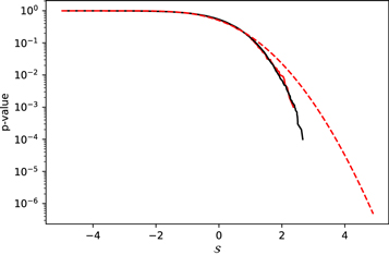
Figure C2. Sky position scramble experiments imposing shuffled anti-HD correlation. For simplicity, we only show the survivor function of  here. The red and black solid curves are measured by evaluating
  with each realization of phase shift with M = 0.1 and 1, respectively. The red dashed curve is for the Gaussian distribution Equation (8).
Download figure:
Standard image High-resolution imageIn addition to the sample space issue, we note that the sky position scrambling operation has two more practical problems and should not be used to evaluate the p-value for our case of  . The first issue is that as the original method Taylor et al. (2017) requires that all realizations are below a certain matching threshold, it is computationally expensive to generate a large number (e.g., ∼104) of samples; if one further requires the noise-weighted threshold (as in general not all pulsars contribute equally due to the differences in their noise properties), the number of independent samples can be further limited (Di Marco et al. 2023). The second issue is that the distribution of
  suffers from fluctuation of individual realizations. We would need thousands of samples to evaluate the statistical threshold for
  . As an example, in Figure C3, we show the survivor function of S from 1000 tries each with 1000 realizations. One can see that the p-value fluctuates from 2 × 10⁻³ to 2 × 10⁻² at
  . Each realization in general over estimate the p-value compared to Equation (8), although a few realizations underestimate the p-value. More than one order of magnitude fluctuation in p-value is noted, for
  . The fluctuation can be even larger, once we allow for a more general form of imposed spatial correlation as explained in the previous paragraph.

Figure C3. 1000 × 1000 sky position scramble experiment imposing shuffled HD correlation. Left: The survivor function of  . Each of the green curves is a single trial with 1000 realizations with M = 0.1. The red dashed curve is for the Gaussian distribution Equation (8). The blue vertical line indicates the
  , while the two black horizontal dashed lines indicate the maximal and minimal p-value at
  found from the green curves, which are 2 × 10⁻² and 2 × 10⁻³, respectively. Right: The scale of p-value fluctuation as a function of
  , computed from the green curves ensembles shown in the left panel. Here, we use the ratio between the maximal and minimal p-value to indicate the fluctuation scale. For
  (blue vertical line), the fluctuation is larger than a factor of 10. In this way, a single trial with 1000 realizations is insufficient to accurately determine the p-value for
  . Significantly more realizations are thus required.
Download figure:
Standard image High-resolution image
One may attempt to remedy the fluctuation by combining the phase shifting and sky position scrambling to produce a larger data set. This will not work in our case, as phase shifting and sky-position scrambling cover different sample spaces. The final p-value calculation depends on the details of how the two methods are combined, which is not meaningful in the statistical modeling.
Due to the results of above experiments and reasons explained, we do not use phase shift or sky-position scrambling to evaluate the p-value of  in the current paper.
Footnotes
- 15
Reconfigurable Open Architecture Computing Hardware: http://casper.berkeley.edu/wiki/ROACH2
- 16
- 17
The 42++ is a PTA data analysis software package developed with the programming language C++ dedicated to the CPTA DR1 analysis. The software is available at https://psr.pku.edu.cn/index.php/publications/gravitational-wave-data-analysis-code/.