
Abstract
We report the properties of more than 600 bursts (including cluster-bursts) detected from the repeating fast radio burst (FRB) source FRB 20201124A with the Five-hundred-meter Aperture Spherical radio Telescope during an extremely active episode on UTC 2021 September 25–28, in a series of four papers. The observations were carried out in the band of 1.0–1.5 GHz by using the center beam of the L-band 19-beam receiver. We monitored the source in sixteen 1 hr sessions and one 3 hr session spanning 23 days. All the bursts were detected during the first four days. In this first paper of the series, we perform a detailed morphological study of 624 bursts using the two-dimensional frequency-time "waterfall" plots, with a burst (or cluster-burst) defined as an emission episode during which the adjacent emission peaks have a separation shorter than 400 ms. The duration of a burst is therefore always longer than 1 ms, with the longest up to more than 120 ms. The emission spectra of the sub-bursts are typically narrow within the observing band with a characteristic width of ∼277 MHz. The center frequency distribution has a dominant peak at about 1091.9 MHz and a secondary weak peak around 1327.9 MHz. Most bursts show a frequencydownward-drifting pattern. Based on the drifting patterns, we classify the bursts into five main categories: downward drifting (263) bursts, upward drifting (3) bursts, complex (203), no drifting (35) bursts, and no evidence for drifting (121) bursts. Subtypes are introduced based on the emission frequency range in the band (low, middle, high and wide) as well as the number of components in one burst (1, 2, or multiple). We measured a varying scintillation bandwidth from about 0.5 MHz at 1.0 GHz to 1.4 MHz at 1.5 GHz with a spectral index of 3.0.
Export citation and abstract BibTeX RIS
Corrections were made to this article on 27 November 2023. A link to the supplementary material has been added.
1. Introduction
Fast radio bursts (FRBs) are radio flashes with a short duration typically in milliseconds (Lorimer et al. 2007). They have a high dispersion measure (DM), exceeding the maximum estimated from the electron column density model (Cordes & Lazio 2002; Yao et al. 2017) for the Milky Way so that almost all of them are considered as extragalactic (Thornton et al. 2013; Cordes & Chatterjee 2019; Petroff et al. 2019; Zhang 2020). Since the discovery of the first event FRB 010724 (Lorimer et al. 2007), hundreds of FRB sources have been discovered. 9 A small number of sources are observed to emit repeated bursts. After the discovery of the first repeater FRB 20121102A (Spitler et al. 2014), a large number of repeated bursts have been detected from 20 FRB repeating sources (CHIME/FRB Collaboration et al. 2019b; Fonseca et al. 2020; CHIME/FRB Collaboration et al. 2021). Recently, a Galactic FRB (dubbed FRB 20200428) was detected from a Galactic magnetar, SGR J1935+2154 (Bochenek et al. 2020; CHIME/FRB Collaboration 2020). Even though its brightness is lower than most extragalactic FRBs, it is orders of magnitude brighter than single pulses of pulsars. The two peaks of the burst also exhibited narrow-band emission characteristics, which is typical for repeating FRBs.
The physical origin and emission mechanism of FRBs are unsolved mysteries (Cordes & Chatterjee 2019; Petroff et al. 2019; Zhang 2020). Hints can be found in the different radiation patterns between the repeaters and non-repeaters. Repeater bursts typically have a narrower frequency band emission and a broader temporal width than non-repeater bursts (e.g., Pleunis et al. 2021). While the lone bursts for non-repeaters prevent detailed studies of non-repeater sources, a large amount of data for repeaters have been collected and analyzed thoroughly. For example, the sub-pulse frequency drifting feature was discovered in many repeated bursts (e.g., CHIME/FRB Collaboration et al. 2019a, 2019b; Hessels et al. 2019; Josephy et al. 2019; CHIME/FRB Collaboration et al. 2020; Day et al. 2020; Fonseca et al. 2020; Li et al. 2021; Platts et al. 2021), which brings interesting constraints on theoretical models (e.g., Wang et al. 2019; Zhang 2022). Sometimes precursors (Hardy et al. 2017; Caleb et al. 2020; Rajwade et al. 2020) or postcursors (Scholz et al. 2017; Gourdji et al. 2019; Cruces et al. 2021) have been detected from some repeaters, i.e., a faint emission component appears prior to or after the brighter primary burst within a very short time from sub-milliseconds to tens of milliseconds, which causes a deviation from the trend of frequency drifting of the bursts.
FRB 20201124A is an active repeater first discovered by CHIME/FRB Collaboration (2021). Similar to FRB 20121102A (Rajwade et al. 2020) and FRB 20180916 (CHIME/FRB Collaboration et al. 2020), a large number of bursts have been detected during the active episode. In the active phase from 2021 March to May, extensive observations (Lanman et al. 2022; Nimmo et al. 2022; Xu et al. 2022) have been carried out. Its location has been well-determined within an arcsecond (Wharton et al. 2021b) by the European VLBI Network (EVN) (Nimmo et al. 2022), which is about 1.3 kpc from the optical center of its host galaxy, SDSS J050803.48+260338.0, a massive star-forming galaxy with a spectroscopic redshift of z = 0.0979 ± 0.0001 (Fong et al. 2021; Piro et al. 2021; Ravi et al. 2022; Xu et al. 2022).
Following-up observations of FRB 20201124A have revealed its various emission characteristics which are similar to other repeaters, such as downward frequency drifting, narrow band emission and scintillation. Based on the observations at 550–750 MHz by the upgraded Giant Metrewave Radio Telescope (uGMRT) and at 1210–1520 MHz by Effelsberg, Main et al. (2022) worked out that the scintillation timescale is τGHz = 0.31 ± 0.06 μs with a best-fit power index of γ=3.5 ± 0.1, lower than 4.0 or 4.4 of the Kolmogorov spectrum. Hilmarsson et al. (2021) discovered circular polarization from one of the bursts and found frequency downward drifting structures of sub-bursts in FRB 20201124A at 1.36 GHz. A persistent radio source, PRS 201124, was subsequently found at the location of this FRB (Ravi et al. 2022), and the spectral energy distribution of the host galaxy is consistent with a star formation galaxy. However, this persistent radio source is extended rather than local to the source (Piro et al. 2021). A bright burst of this repeater had a flux density of 0.7 ± 0.01 mJy at 650 MHz as detected by uGMRT (Wharton et al. 2021a) and 0.34 ± 0.03 and 0.15 ± 0.01 mJy at 3 and 9 GHz as detected by the VLA (Ricci et al. 2021).
As the largest and most sensitive single antenna radio telescope in the world, the Five-hundred-meter Aperture Spherical radio Telescope (FAST, Nan et al. 2011) is an ideal facility for detecting weak radio signals from FRBs (Luo et al. 2020; Li et al. 2021; Niu et al. 2022a) and pulsars (Han et al. 2021). It can track sources well with a pointing accuracy of 8 arcseconds (Jiang et al. 2020) and record polarization signals in the pulsar search mode (Han et al. 2021). During the active period of FRB 20201124A from 2021 April 1 to June 11, Xu et al. (2022) reported the detection of 1863 bursts. Based on the analysis of recorded polarized signals, they revealed rich features from this large sample of bursts, including detecting significant variations of the Faraday rotation measures and the oscillation features of the polarization properties with respect to wavelength in a small fraction of bursts.
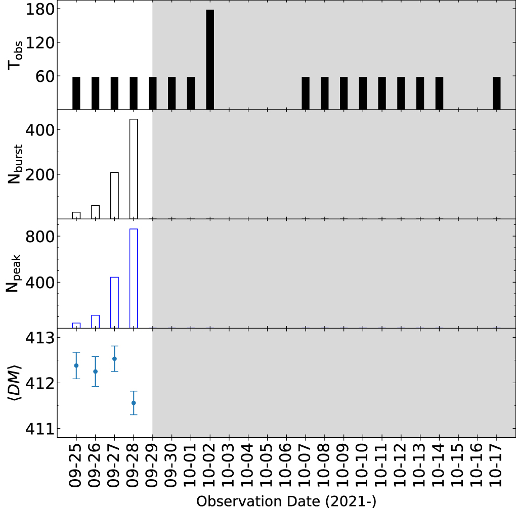
Triggered by the Canadian Hydrogen Intensity Mapping Experiment (CHIME) detection 10 and the report by Main et al. (2021), we started to monitor FRB 20201124A with FAST on 2021 September 25 and continued to monitor the source almost daily until October 17. A large number of bursts have been detected in the first 4 days (see Figure 1) with very diverse emission properties. In this paper, we focus on the burst morphology and taxonomy of more than 600 detected bursts or cluster-bursts. Their energy distribution is discussed in Paper II (Zhang et al. 2022); the polarization properties are analyzed in Paper III (Jiang et al. 2022); and the bursts arrival time is analyzed in Paper IV (Niu et al. 2022b). In Section 2, we briefly introduce the FAST observations and burst detection. The detailed analysis methods are presented in Section 2.1. DM measurements and parameter determination for emission frequency peak and emission bandwidth, sub-burst width and fluence are presented in Sections 2.2 and 2.3. The statistics of burst parameters and morphology classifications are presented in Section 3. Finally, the summary is presented in Section 4 and the comparison of observational results with other repeating sources are discussed there.

Figure 1. FRB 20201124A was monitored from 2021 September 25 to October 17 by FAST. The panels from top to bottom show the observation duration (in minute) each day, numbers of detected bursts, numbers of fitted peaks and averaged DMs (in pc cm−3) respectively. The gray shaded area indicates no bursts detected from the FAST observations for many days. See the relevant numbers in Table 1.
Download figure:
Standard image High-resolution image2. Observations and Burst Detection
After FRB 20201124A was found to be active again by the CHIME and Effelsberg Telescope (Main et al. 2021), we started the monitoring program by FAST at the coordinate of R.A. = 05h08m03 5077, decl. =
  for FRB 20201124A obtained by the European Very Long Baseline Interferometry Network (EVN) (Marcote et al. 2021), and scheduled 17 effective FAST observations of FRB 20201124A from 2021 September 25 to October 17.
The central beam of the L-band 19-beam receiver is used to cover the frequency range from 1.0 to 1.5 GHz (Jiang et al. 2020; Li et al. 2018). Our FAST observations were carried out for one hour each day, except for three hours on 2021 October 3. The calibration signals of periodic noise are injected for 1 minute at the beginning and the end of each observation, so that data on the source are effectively 58 minutes. The four polarization channels (XX, YY, XY*, X*Y) are sampled with a time resolution of 49.152 μs by the digital backend in pulsar searching mode, using 4096 frequency channels (0.122070 MHz each channel) to cover 1.0 to 1.5 GHz. The data are stored in PSRFITS format (Hotan et al. 2004), and each FITS file records data of about 12.88 s. The observation setup details are as same as the first FAST monitoring session in 2020 April–May (Xu et al. 2022).
2.1. Data Analysis and Burst Detection
An independent data analysis for searching single pulses is carried out by the first author of this paper. The discovered bursts are verified by members of other groups in the author list, as are also reported in other papers of this series.
Before the single pulse search, all small FITS files, of which each consists of 12.88 s observation data, are merged to a single FITS file in the chronological order. To reduce the file size, 256 out of 4096 frequency channels at each edge of the L-band that have a very low gain are discarded, thus a 31.25 MHz band on each side of the band is cut off. The power of XX and YY of other frequency channels are then combined, and the channel number and sampling time are reduced by a factor of 8 and 4, respectively. The total power for a total of 448 (rather than 512, reduced by a factor of 8) frequency channels with a sampling time of 49.152 × 4 μs (i.e., downsampling by a factor of 4) are prepared for the following single pulse detection. If a pulse is detected, the original raw data for all channels are analyzed for pulse properties.
Specifically for FRB 20201124A, we search pulses in a few steps. First of all, we dedisperse data in the range of 3–1000 cm−3 pc in steps of 1.0 cm−3 pc to form two-dimensional images on the time versus DM. An artificial intelligence (AI) approach is carried out in the GNU Parallel (Tange 2020) to identify dedispersed pulses. Some frequency channels always with strong Radio frequency interference (RFI) are discarded during this process. To improve the pulse detection, we divide 448 channels into two parts, the upper half and lower half of the total band, and perform the single pulse search separately. We also search pulses in the upper and lower quarter of 448 channels. Any pulse candidates with signal-to-noise ratio (S/N) > 7 are manually viewed and checked further in the two-dimensional frequency-time water-fall plots.
In an earlier FAST paper reporting the previous active episode of the source (Xu et al. 2022) and that in Paper II (Zhang et al. 2022), the waiting time distribution of dedispersed emission peaks from FRB 20201124A exhibits two wide peaks, one from a few ms to a few tens of ms, and the other from a few seconds to a few tens of seconds. The first peak may indicate several emission components occurring in one burst, while the second peak probably stands for the interval between two adjacent independent bursts. The valley between the two peaks of the waiting time distribution can be used to distinguish independent bursts. Based on the waiting time distribution, we take the separation of 400 ms between any of two emission components as indication for the another independent burst. This allows us to better characterize and compare the emission morphology of the emission peaks within the same emission episodes. More specifically, we adopt the following definitions for the terminology:
- 1.
- 2.A sub-burst stands for one of several more or less connected components in the frequency-time waterfall plots (see Figure 2) generally within a few tens of milliseconds, and it has a distinguished peak in the dedispersed burst profile.
- 3.A cluster-burst is defined as a collection of several somehow independent bursts with a separation less than 400 ms, but there is no bridge emission in between since the burst intensities come back to the system noise level.
We note that the definitions of the bursts are somewhat different in other papers in the series. This is because different papers have different scientific purposes and the lead authors defined their "bursts" for the convenience of conducting their respective analyses. Therefore, the numbers of "bursts" reported in different papers are somewhat different, even though the same data set has been analyzed.

Figure 2. The dynamic spectra of four bursts illuminating the difficulty to determine DMs. In the upper sub-panel of each plot is the frequency-time water-fall plot, and the average burst profile over all frequency channels is shown in the bottom sub-panel. The observational date and the time of arrival (TOA) in MJD are marked on the top of each plot. The burst number on that day and burst width in ms, together with the DM value used and the total fluence of this burst are marked in the lower-sub-panel. In the top three panels, the DM values of bursts No. 33 and No. 35_A and No. 144_A on 20210927 are determined from burst emission at the upper half band of the FAST observations, and the middle panels are the same data but with DMs determined from the emission at the lower half band. The wide panel in the bottom shows a complex, No. 113 on 20210927, which have many sub-bursts so that it is difficult to obtain one DM to align with all the burst emission. We then have to compromise by using the averaged DM of the day to generate this plot.
Download figure:
Standard image High-resolution imageWe obtained 29, 57, 169, and 369 bursts in the first 4 days, respectively, and in total 624 bursts from FRB 20201124A during this active episode. A full list of the bursts (see Table A1) together with plots for each bursts (see Figures A4–A13) are presented in the
Table 1. Observation Sessions and Detected Bursts
| Date | Tobs | Burst | Burst Rate | Peak | 〈DM〉 (σ) |
|---|---|---|---|---|---|
| (min) | No. | (hr−1) | No. | (cm−3pc) | |
| 20210925 | 58 | 29 | 30.0 | 44 | 412.4(3) |
| 20210926 | 58 | 57 | 60.0 | 111 | 412.2(3) |
| 20210927 | 58 | 169 | 174.8 | 441 | 412.5(3) |
| 20210928 | 58 | 369 | 381.7 | 865 | 411.6(3) |
| 20210929 | 58 | 0 | 0 | 0 | |
| 20210930 | 58 | 0 | 0 | 0 | |
| 20211001 | 58 | 0 | 0 | 0 | |
| 20211002 | 178 | 0 | 0 | 0 | |
| 20211007 | 58 | 0 | 0 | 0 | |
| 20211008 | 58 | 0 | 0 | 0 | |
| 20211009 | 58 | 0 | 0 | 0 | |
| 20211010 | 58 | 0 | 0 | 0 | |
| 20211011 | 58 | 0 | 0 | 0 | |
| 20211012 | 58 | 0 | 0 | 0 | |
| 20211013 | 58 | 0 | 0 | 0 | |
| 20211014 | 58 | 0 | 0 | 0 | |
| 20211017 | 58 | 0 | 0 | 0 |
Download table as: ASCIITypeset image
2.2. The Most Probable DM Value
The bursts of FRB 20201124A detected by the FAST show various dynamic spectra structures. They are detected first with a given DM value. However, when the detailed structures are studied, a proper DM is the key to determine the physical properties of the bursts (see Figure 2).
Following the approach for other FRBs in the literature (CHIME/FRB Collaboration et al. 2019b; Marthi et al. 2022; Xu et al. 2022), we first use the package DM_phase 11 to find the best DM for every burst. This handy program can find the best frequency alignment of de-dispersed sub-burst features.
For bursts of FRB 20201124A, however, the outcomes of DM_phase need to be taken with caution. It gives a very reasonable result for some bursts, but not for all, mainly because of the complicated burst properties of FRB 20201124A. After examining the determined DMs and the waterfall plots for all bursts, we found that it is hard to make a good and uniform standard to determine the DMs for various bursts. Figure 2 shows some examples of the dilemma. The burst No. 33 on 20210927 shows a more reasonable DM determined from the upper half-band by using DM_phase, while it is reversed for the bursts No. 35_A and 144_A on 20210927. If one takes the leading component of the burst No.35_A as an independent burst (see Figure 2), DM_phase would derive a DM that is so large that this burst appears to have its lower part distorted toward earlier time in the water-fall plot, rather than simply vertically aligned. We get many similar cases. This fact suggests that the bursts of FRB 20201124A almost always have an intrinsic downward frequency drifting.
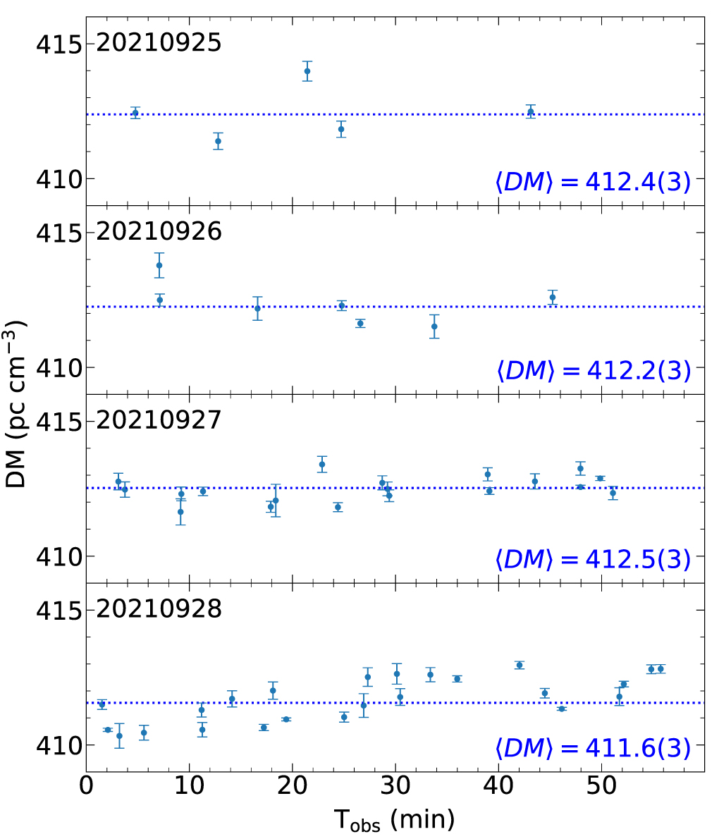
For this session of FRB 20201124A, we have to determine the DMs only for a small number of selected bursts which we feel confident in the DM results from DM_phase, having either a significant inter-structural gap as No. 15 on 20210925 in Figure 3 or a sharp leading edge as No. 228 on 20210928. With some well-determined DMs of a small fraction of bursts in Figure 4, we see the insignificant DM variation in about one hour each day, and the averaged DM values are consistent with each other on the first three days. A slightly smaller averaged DM value and a weaker trend of DM increasing is seen on the last day 20210928.
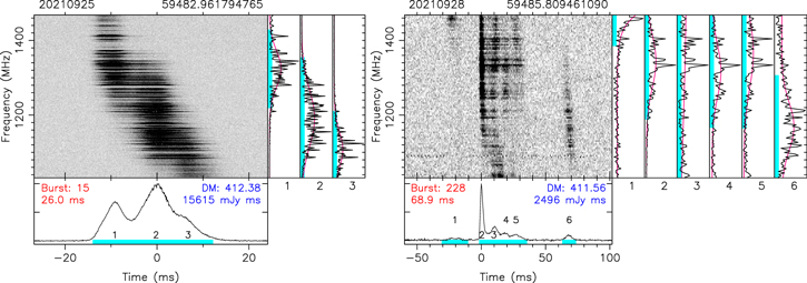
Figure 3. The dynamic spectra of two bursts with DM values well determined by the DM_phase package. In the bottom sub-panel, the sub-burst numbers are marked. Their energy distributions over frequency are shown in the right sub-panels and fitted with a Gaussian function to obtain the emission peak frequency ν0 and emission bandwidth BWe.
Download figure:
Standard image High-resolution image
Figure 4. DM values are confidently determined for a number of bursts using the package DM_phase, with the mean DM values marked for each day.
Download figure:
Standard image High-resolution imageIn the following analyses, the averaged DM for each day is adopted for data analyses. There is no question that a different DM would cause a different drifting rate, but we do not have a better choice at present.
2.3. Burst Parameters
We measured the observational parameters of 624 bursts, such as the TOA expressed in MJD for the peak of the each sub-burst, the emission peak frequency (ν0, in MHz), the sub-burst emission bandwidth (BWe, in MHz), the sub-burst width (Wsb, in ms), the detection S/N, and the fluence of a bursts or a sub-burst (Fν
, in mJy ms). All these parameters are listed in Table A1 in the
For each burst, we dedisperse the data by using the average DM value each day and obtain a burst profile first from an obvious frequency range manually selected, because most bursts have emission merely in some parts of the observation band of 500 MHz of the FAST L-band receiver, see examples in Figure 3 and plots for all bursts in the
For each sub-burst, the TOA is defined as the arrival time of the emission peak at the infinity frequency. The peak is obtained from the Gaussian function fitted to the de-dispersed burst profile. There are 44, 111, 441 and 865 sub-burst peaks in the first 4 days, respectively, and in total 1459 peaks. The TOA is then converted to the solar barycentric center using the DE438 ephemeris.
The sub-burst width Wsb is defined as the full width of 10% of maximum (FWTM) measured from a fitted Gaussian function to the dedispersed profile of a sub-burst. The burst width Wb is then defined as the overlapping width of these fitted multi-Gaussian functions for all sub-bursts with the 10% of maximum of two Gaussian functions for the two outermost components. The signal-to-noise ratio (S/N) is calculated from the summed energy of the fitted Gaussian profile relative to the standard deviation (σ) obtained from the nearby off-pulse ranges with a similar width of a burst.
The fluence of a burst or sub-bursts, Fν in units of mJy ms, is estimated from the above-defined sub-burst parameters and the system characteristics, via

here ∑ Si is the summed value of on-burst bins, Tsys = 25 K is the system noise temperature, and G0 = 16.1 K Jy−1 is the effective gain of the telescope (Jiang et al. 2020), np = 2 is the number of polarization summed, tsamp is sampling time (s), and BWe is emission frequency bandwidth (MHz) obtained above.
3. Burst Morphology and Classification
As shown in the plots for 624 bursts in Figures A4 to A13, the burst emission detected by the FAST always has a narrow band, sometimes detected only in the lower or upper edges of the FAST band of 500 MHz, occasionally with a wide-band covering all the band. Another interesting phenomenon, as burst No.15 in Figure 3 shows, is that a burst emission starts to appear in the upper band, and slightly later a new component emerges in the central band, and then another new component comes later in the lower band. This is the so-called downward frequency drifting of burst emission (Hessels et al. 2019). With such a large sample of detected bursts and their characteristics, the bursts can be classified according to their morphology in the time-frequency waterfall plots. In this section, we first analyze the frequency distribution of the burst emission, then discuss the drifting patterns, and finally classify the bursts based on morphology.
3.1. Burst Parameters Distributions
After obtaining the burst parameters, i.e., emission peak frequency ν0 and the emission bandwidth BWe, sub-burst width Wsb and fluence Fν of every sub-burst of all bursts, we perform a statistics quantitatively for these parameters in Figure 5. Due to the limitation of the FAST observation bandwidth, some fitted ν0 for the sub-bursts emerging near the band edges have the best fitted value outside the FAST frequency range or just near 1080 or 1420 MHz but with a BWe < 150 MHz. These account for 21% of the total sub-bursts. The fitted parameters for these 21% sub-bursts are unusual and have a large uncertainty and are therefore dropped. The remaining approximately 79% of data as indicated by the blue symbols in Figure 5 are used for the statistical analysis.

Figure 5. Data distributions of emission peak frequency (ν0), burst emission bandwidth (BWe), sub-burst width Wsb and specific fluence Fν of all sub-bursts of FAST detected bursts. The values are estimated via Gaussian fittings, with a relative uncertainty less than 10%. The blue dots stand for good values obtained from the fittings (see Section 2.3). The gray crosses stand for data with ν0 outside the frequency range or that BWe < 150 MHz but ν0 lower than 1080 MHz or higher than 1420 MHz. The vertical dashed lines indicate the effective observational frequency range of the FAST from 1031.25 to 1468.75 MHz. A few points with Wsb > 30 ms are not included. The histogram of ν0 distributions shows two peaks, which are fitted with two Gaussian functions peaking at 1901.9 MHz and at 1327.9 MHz. The histogram of BWe and Wsb distributions can be fitted by a log-normal function, and they peak at 277 MHz and 7.4 ms, respectively. The histogram of the log Fν distribution has a dip near the peak but can be fitted with two Gaussian functions with peaks at log Fν = 2.1 ± 0.3 and log Fν = 2.9 ± 0.4, respectively. It is noticed that the sub-burst width Wsb tends to be larger for the bursts emerging at the lower part of the band, while the emission bandwidths BWe of these bursts tend to be smaller than the bursts emerging at high frequency part of the band, as illustrated by the median and the standard deviation for the three sub-bands in the first column of data distribution of ν0 vs. BWe and distribution of ν0 vs. Wsb.
Download figure:
Standard image High-resolution imageFirst of all, we notice that there are two peaks in the histogram of the ν0 distribution, which are at 1091.9 MHz and 1327.9 MHz as the Gaussian fitting gives, and the standard deviation σ of the Gaussian distribution is 62.0 MHz and 113.0 MHz, respectively. The number of sub-bursts distributed in the lower-frequency component is larger, suggesting that this FRB source preferably emits at the lower part of the FAST band.
One may question if the two peaks of the ν0 distribution in Figure 5 are caused by removing the strong Radio frequency interference (RFI) around 1250 MHz within the observation bandwidth of FAST. Because RFI appears mostly in a few tens of MHz in the central part of the observation band, the emission strength of the bursts from channels in the two sides of the RFI bands is not affected. Because the emission bandwidth is as wide as more than 200 MHz, discarding some channels with RFI does not affect the fitting results for both ν0 and BWe. This has also been verified by simulations (not presented in this paper).
The emission bandwidth BWe in Figure 5 follows a log-normal distribution with a peak at about 277 MHz. The borderlines of the full width half maximum of the emission bandwidth are at about 193 MHz and 399 MHz, narrower than the FAST observed bandwidth.
The sub-burst width Wp
in Figure 5 also follows a log-normal distribution concentrated in the range of 1 to 30 ms, with a peak at about  ms. We notice that sub-burst width is wider for the bursts emerging at the lower part of the band. We divide the band into three sub-bands centered at 1104.2 MHz, 1250.0 MHz and 1395.8 MHz, and found that sub-burst widths have median values of Wsb of 9.8 ± 4.3 ms, 8.8 ± 4.2 ms and 7.1 ± 3.9 ms, respectively, for the sub-bursts peaking in these three sub-bands. On the other hand, the emission bandwidth becomes wider for the sub-bursts emerging at the higher part of the band, i,e, BWe = 270.4 ± 108.3 MHz, 362.8 ± 131.2 MHz and 367.3 ± 148.2 MHz for the three sub-bands. The correlation coefficient between ν0 and Wsb is −0.25 and that between ν0 and BWe is 0.36.
The distribution of sub-burst specific fluence Fν has a dip near the peak but can be roughly fitted with two Gaussian functions in the logarithmic scale, peaking at logFν = 2.2 ± 0.3 and logFν = 2.9 ± 0.3. Details of the energy distribution of FRB 20201124A are discussed in Paper II (Zhang et al. 2022).
3.2. Frequency Drifting of Bursts
An important feature of FRB 20201124A is the time-frequency drifting pattern clearly shown in most bursts, not only for bursts with multiple components, but also for single component bursts. In the literature (Gajjar et al. 2018; CHIME/FRB Collaboration et al. 2019a; Hessels et al. 2019; Hilmarsson et al. 2021), frequency drifting was always discussed for the bursts with multiple components and the authors defined the shift of sub-bursts in the 2D frequency and time domain. Our observations of FRB 20201124A in Figures A1–A4 show that even the bursts with a single component also have a clear drifting pattern when the front edge of burst is aligned with the average DM, as shown in the example presented in Figure 6.

Figure 6. An example of frequency drifting for a single-component burst, i.e., burst No. 218 detected on 20210928. The top panel in Figure 3 is the dynamic spectrum. The front edge of this burst is aligned well with the average DM of the day. The emission bandwidth of the burst BWe, as marked in the top-right sub-panel, is cut to three sub-bands, and the relative TOAs of the burst are obtained respectively for the frequency-scrunched profiles of the three sub-bands, as shown in the bottom panel. The downward frequency drifting rate is then found to be Rd = −66 ± 8 MHz ms−1. The thick solid line stands for the best-fitting result, and the dotted lines in black indicate the range of uncertainty.
Download figure:
Standard image High-resolution imageFirst we look at drifting of single component bursts. We cut the emission band of the burst BWe to three sub-bands, then get three averaged burst profiles from each sub-band, and obtain the TOAs of sub-burst peaks with Gaussian fitting. The drifting rate, Rd in MHz/ms, is obtained as the slope of the least square fit to TOAs for the three sub-bands, as demonstrated in Figure 6. The drifting rate Rd depends on the implemented DM value for the burst, and the data in Table 2 are obtained with the average DM of the day. The uncertainty of Rd depends on the uncertainty of the central frequency and the TOAs in each sub-band. In principle, we can measure Rd for each sub-burst. Nevertheless, to examine how the bursts drift, we choose only 31 single-component bursts with BWe > 250 MHz and burst detection S/N > 50. Their drift rates Rd are listed in Table 2 and plotted against the emission peak frequency in Figure 7.

Figure 7. The drifting rate distribution of single-component bursts (top panel) and multi-component bursts (bottom panel) listed in Table 2, plotted against the emission peak frequency.
Download figure:
Standard image High-resolution imageTable 2. Drifting Rate Rd of Single-component Bursts and Multi-component Bursts
| Date | Burst | No. | ν0 | BWe | Rd (err) |
|---|---|---|---|---|---|
| No. | Comp. | (ms) | (MHz) | (MHz ms−1) | |
| Single component bursts | |||||
| 20210925 | 8 | 1 | 1153.8 | 89.5 | −58(7) |
| 20210926 | 9 | 1 | 1188.8 | 118.8 | −64(8) |
| 20210927 | 54 | 1 | 1151.3 | 73.1 | −95(12) |
| 20210927 | 80 | 1 | 1124.9 | 81.9 | −59(7) |
| 20210927 | 87 | 1 | 1127.5 | 101.5 | −54(7) |
| 20210927 | 125 | 1 | 1250.7 | 118.4 | −77(10) |
| 20210927 | 138 | 1 | 1057.3 | 70.8 | −55(7) |
| 20210928 | 3 | 1 | 1146.2 | 80.4 | −58(7) |
| 20210928 | 39 | 1 | 1280.2 | 118.8 | −68(9) |
| 20210928 | 46 | 1 | 1367.0 | 69.1 | −166(18) |
| 20210928 | 61 | 1 | 1249.7 | 118.7 | −36(4) |
| 20210928 | 112 | 1 | 1383.2 | 105.5 | −58(7) |
| 20210928 | 125 | 1 | 1342.4 | 118.8 | −78(10) |
| 20210928 | 143 | 1 | 1151.2 | 79.3 | −41(5) |
| 20210928 | 154 | 1 | 1413.9 | 89.0 | −62(7) |
| 20210928 | 162 | 1 | 1204.3 | 118.8 | −104(13) |
| 20210928 | 179 | 1 | 1165.0 | 74.0 | −52(6) |
| 20210928 | 187 | 1 | 1129.1 | 73.8 | −93(12) |
| 20210928 | 189 | 1 | 1260.1 | 117.5 | −62(8) |
| 20210928 | 197 | 1 | 1174.1 | 81.9 | −61(5) |
| 20210928 | 210 | 1 | 1192.6 | 98.0 | −66(8) |
| 20210928 | 220 | 1 | 1269.4 | 91.2 | −128(17) |
| 20210928 | 236 | 1 | 1160.2 | 81.9 | −28(3) |
| 20210928 | 275 | 1 | 1217.6 | 107.4 | −104(14) |
| 20210928 | 276 | 1 | 1135.2 | 77.2 | −54(7) |
| 20210928 | 280 | 1 | 1333.2 | 73.5 | −74(9) |
| 20210928 | 286 | 1 | 1215.1 | 99.9 | −50(6) |
| 20210928 | 291 | 1 | 1256.5 | 118.8 | −86(11) |
| 20210928 | 298 | 1 | 1351.3 | 84.0 | −74(9) |
| 20210928 | 355 | 2 | 1398.0 | 74.7 | −42(5) |
| 20210928 | 369 | 1 | 1298.2 | 92.6 | −90(12) |
| Multiple component bursts | |||||
| 20210925 | 15 | 1–3 | 1323.6 | 89.1 | −14(2) |
| 20210926 | 5 | 1–4 | 1440.3 | 104.9 | −18(2) |
| 20210926 | 22 | 1–4 | 1254.7 | 51.2 | −6(4) |
| 20210927 | 59 | 1–4 | 1426.3 | 72.3 | −17(7) |
| 20210927 | 75 | 1–4 | 1356.7 | 96.0 | −29.0(6) |
| 20210927 | 111 | 1–3 | 1473.0 | 127.7 | −28(6) |
| 20210927 | 165 | 1–4 | 1407.4 | 85.5 | −18(2) |
| 20210928 | 3 | 4–6 | 1153.1 | 34.5 | −5(3) |
| 20210928 | 182 | 1–3 | 1361.7 | 118.4 | −23(5) |
| 20210928 | 186 | 1–4 | 1387.2 | 86.9 | −28(3) |
| 20210928 | 267 | 1–3 | 1411.0 | 90.6 | −21(2) |
| 20210928 | 296 | 1–4 | 1402.9 | 101.8 | −19(5) |
Download table as: ASCIITypeset image
For multi-component bursts, we selected 12 bursts with at least three sub-bursts. Each sub-burst is taken as a component to obtain the central emission frequency ν0 and the TOA of the frequency scrunched profiles, e.g., the multi-component burst No. 15 on 20210925 in the left panel of Figure 3. The precursor and post-cursor near the band edges are excluded. We confidently obtain the frequency drifting rate for these 12 multi-component bursts listed in Table 2 and their values are also plotted against the emission peak frequency in Figure 7.
As listed in Table 2 and seen in Figure 7, all confidently and quantitatively derived frequency drifting rates have negative values, which indicates the downward frequency drifting of bursts. The drifting rate is plainly understandable in the frequency-time waterfall plot, though the exact values depend on the implemented DM value. As seen in Table 2, the drifting rates for very carefully selected single-component bursts are in the range between −166 and −28 MHz ms−1, and their average value is −61 ± 9 MHz ms−1. The drifting rates for multi-component bursts represent the average delay of several components in different parts of the frequency band, hence they have much lower values than those of single-component bursts. The drifting rates for multi-component bursts are in the range from −29 to −5 MHz ms−1, with an average value of −21 ± 4 MHz ms−1. This is only about one third of the drifting rate for single-component bursts. The bursts emerging in the higher half band tend to have a larger drifting rate than those detected only at the lower part of frequency band.
3.3. Burst Morphology Classification
With the implemented daily-average DM to all the bursts, one can systematically study the burst morphology. One immediate observation is that the bursts show a diverse morphology. The primary features of the bursts are the frequency drift and the limited emission band. The number of sub-bursts, i.e., the component of burst profiles, is another interesting feature. We therefore can classify the detected bursts from FRB 20201124A based on these key features.
First of all, based on the frequency drifting, more than half of 624 bursts have shown a downward frequency drifting feature in the waterfall plots. Only a few cases show an upward drifting feature. The remaining bursts are either complex, show no drifting with the given DM, or have no evidence for drifting due to the limited emission bandwidth caught by FAST. Second, only a small fraction of bursts, which we categorize as "wide-band", are detected in the entire FAST observation band. Most of the bursts are detected only in a narrow part of the FAST L-band of 1.0–1.5 GHz, either in the high frequency part, the middle part, or the lower part. Therefore, the sub-classes can be distinguished according to the emission band where the bursts appear. Moreover, for the downward drifting bursts, the sub-classes can be further grouped according to the number of burst components. See Table 3 for the number of bursts in each class or sub-class. Examples are shown in Figure 8 for the dynamic spectrum of frequency downward-drifting bursts with one (in the left column panels), two (in the middle column panels) and multiple components, with their emission seen in wide-band, high-frequency, middle-frequency band, or low-frequency part of the FAST band (from top to bottom).
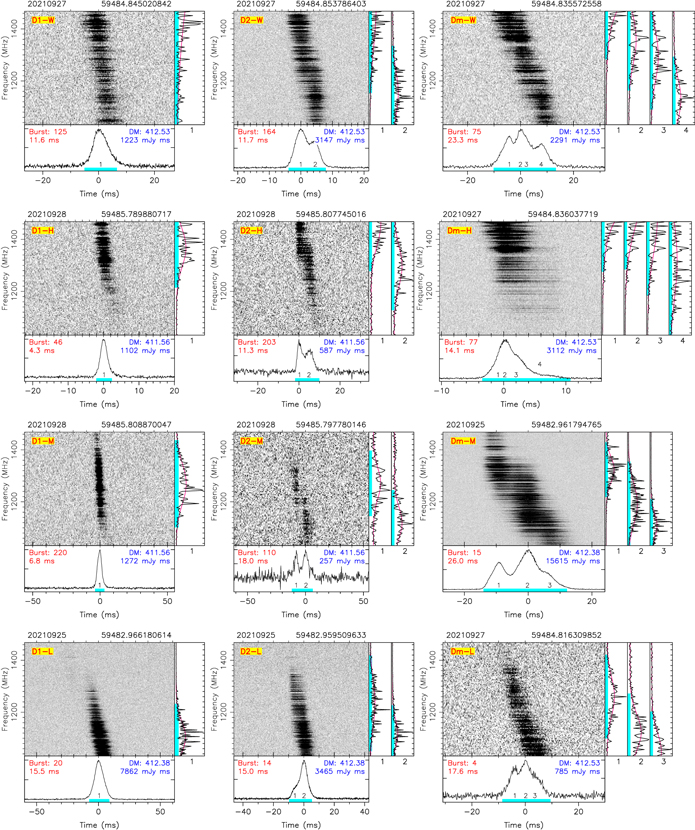
Figure 8. Dynamic spectra for frequency downward-drifting bursts with one (in the left column panels), two (in the middle column panels) and multiple components, and their emission is shown in the wide-band, the high part, the middle part, or the lower part of the FAST band (from top to bottom). The plot for each burst includes not only the water-fall plot but also the frequency-scrunched burst profile in the bottom sub-panel, with the number of the profile components and burst width marked. In the left sub-panels are the burst energy distribution over frequency for each component, fitted with Gaussian functions, with the effective emission bandwidths being marked. The observation date and the TOA of the burst peak are marked on the top of the water-fall plot, and the classification of each burst is marked on the plot. The burst number and burst width, as well as the DM and fluence are marked in the lower sub-panel.
Download figure:
Standard image High-resolution imageTable 3. Classification of the Bursts and the Detected Burst Numbers for Each Category for the Burst Detected in this 2021 September (25–28) Active Episode
| Drifting mode | Component | Burst emission emerging in the frequency band | |||
|---|---|---|---|---|---|
| No. | Wide band | High part | Middle part | Lower part | |
| Downward: 263 | |||||
| one | D1-W: 18 | D1-H: 16 | D1-M: 31 | D1-L: 68 | |
| two | D2-W: 22 | D2-H: 14 | D2-M: 11 | D2-L: 48 | |
| multiple | Dm-W: 14 | Dm-H: 6 | Dm-M: 8 | Dm-L: 7 | |
| Upward: 3 | U-H: 1 | U-L: 2 | |||
| No evidence: 121 | NE-H: 10 | NE-L: 111 | |||
| No Drifting: 35 | ND: 35 | ||||
| Complex: 203 | C: 203 (including 157 cluster-bursts) | ||||
Download table as: ASCIITypeset image
In the following, we briefly discuss each class and sub-class of bursts.
3.3.1. One-component Bursts with Downward Frequency Drifting: D1-W, D1-H, D1-M and D1-L
D1-W: Only a few percent of bursts show wide-band emission, with an emission bandwidth larger than 500 MHz of the FAST observations. The integrated burst profile has a single component. If the waterfall plot is forced to be aligned to get a DM value, the emission at the lower part of the band would be distorted due to a slightly larger DM from the alignment (see the separated leading component of burst No. 35 in Figure 2). With the average DM of the day, we get 18 such one-component downward-drifting bursts, as shown in Figure A1.
D1-H: There are 16 one-component bursts in Figure A2 which have emission only in the higher frequency part of the FAST band, showing the downward frequency drift pattern.
D1-M: There are 31 one-component bursts in Figure A3 which have emission only in the middle part of the FAST observation band.
D1-L: There are 68 one-component bursts in Figure A4 which have emission only in the lower part of the band, with the emission peak frequency near or below the FAST lower band limit. Some bursts have much extended emission toward the band lower limit, which also indicates the trend of frequency downward drifting, even though a quantitative analysis would be difficult.
3.3.2. Two-component Bursts with Downward Frequency Drifting: D2-W, D2-H, D2-M and D2-L
The two-component bursts are practically the same as the one-component burst, except that two sub-pulses are observed within 50 ms. For a longer separation, they would be considered as independent bursts or a burst with precursor or postcursor. The burst profiles can be fitted with two Gaussian functions. There are 22, 14, 11 and 48 bursts in the sub-classes of D2-W, D2-H, D2-M and D2-L, respectively. See Figures A5 to A8 for their plots. The longer tails of D2-L bursts cannot be well distinguished from the scattering tail of some bursts.
3.3.3. Multi-component Bursts with Downward Frequency Drifting: Dm-W, Dm-H, Dm-M and Dm-L
Multi-component bursts have three or more components in the burst profiles, and the downward drifting occurs between these components, as discussed above. These bursts can appear in the wide-band, or in the high part, middle part, or the lower part of the FAST band, as shown in Figures A9–A12. There are 14, six, eight and seven bursts in each of these sub-classes, respectively.
3.3.4. Upward Frequency Drifting Bursts
Three bursts have the second or the third component appearing at a higher frequency band than the first one, so that they look like an upward frequency drifting as shown in Figure 9. One of them have emission in the higher part of the band, denoted as subclass U-H, and two of them have emission in the lower part of the band, denoted as subclass U-L.

Figure 9. Same as Figure 8 but for upward drifting of bursts with two or three components, i.e., the later component has a higher emission peak frequency than the first one.
Download figure:
Standard image High-resolution image3.3.5. Bursts with no Evidence for Drifting
Some bursts emerge near the edges of FAST observation band, either the higher or lower edge. The burst emission band is too narrow to determine whether there is a frequency drifting pattern. We classify these bursts as "No evidence" for drifting. They are further classified as NE-L (111 bursts) or NE-H (10 bursts) as their emission emerges in the lower or higher part of the FAST frequency band, respectively. See Figures A13 and A14 for the plots.
3.3.6. No Drifting Bursts
Dynamic spectra of 35 bursts (see Figure A15) manifest a very vertically pattern, with their emission band wide enough to clearly judge that there is no frequency drifting (ND), regardless whether the emission appears at high, middle or low part of the frequency band.
3.3.7. Complex
There are 203 bursts, including 157 cluster-bursts (see Figure A16), which have many interesting burst components showing complex structures in the waterfall plots, either a mixture of upward and downward drifts or a mixture of individual downward drifts with precursors or postcursors in a short time or a cluster burst. It is really worth reading all plots in Figure A16. The burst No. 113 on 20210927 in Figure 2 is an extreme case of complex bursts, which has the longest continuous emission duration (120 ms) with at least 10 burst components one after another. Some of them show upward drifting, but some others show downward drifting patterns.
4. Discussion and Conclusions
We report above the FAST detections of 624 bursts from FRB 20201124A in a star-forming galaxy at z = 0.0979 during an extremely active episode in the end of 2021 September. On 2021 September 28, the burst rate was 381.7 hr−1, which is the highest among known FRB repeaters. The source was then suddenly quenched, with no bursts detected in the following three weeks. In our morphological study, we define a burst as an emission episode during which the adjacent emission peak separation is shorter than 50 ms. The sub-bursts coming in such a duration are then counted as components of a burst. If all the components are counted as independent bursts, we would get 1461 bursts in total, which almost double the number of the bursts claimed in this paper.
The morphology of detected bursts of FRB 20201124A is diverse and intriguing. Most bursts are emitted in a relatively narrow frequency range inside the FAST observation band, and their energy distribution over frequency can be fitted with a Gaussian function. The typical emission bandwidth is  MHz, as described in Section 3.1. The emission peak frequency ν0 has a distribution in the FAST observation band, which can be fitted with two Gaussian functions, one with 1091.9 ± 62.0 MHz and the other with 1327.9 ± 113.0 MHz. Some bursts have emission detected only in the higher frequency part of the band, some in the middle, and some others in the lower frequency part of the observation band. A small fraction of bursts have wide band emission and are detected in the entire FAST band. The sub-burst widths (Wp
) of the bursts have a wide distribution of
MHz, as described in Section 3.1. The emission peak frequency ν0 has a distribution in the FAST observation band, which can be fitted with two Gaussian functions, one with 1091.9 ± 62.0 MHz and the other with 1327.9 ± 113.0 MHz. Some bursts have emission detected only in the higher frequency part of the band, some in the middle, and some others in the lower frequency part of the observation band. A small fraction of bursts have wide band emission and are detected in the entire FAST band. The sub-burst widths (Wp
) of the bursts have a wide distribution of  ms. Downward frequency drifting is observed from more than half of the detected bursts, including both one-component and multi-component bursts. Based on the burst features in the dynamic spectra of the frequency-time waterfall plots, the bursts of FRB 20201124A are classified into 18 groups. The complex features of some bursts are caused by the intrinsic emission properties of the FRB, rather than by its environment. This is because the variation of morphology occurs among sub-bursts of one single burst and the time is too short to introduce a large DM variation due to varying free electron column density along the line of sight.
In the following, we compare the frequency drifting properties of FRB 20201124A with other FRBs in detail, and then discuss the scintillation-induced emission intensity fluctuations.
4.1. Frequency Drifting and Radiation Mechanisms
Frequency drifting structures have been observed in many FRB bursts, e.g., FRB 121102, FRB 180814.J0422+73, FRB 180916.J0158+65 and FRB 190711 (Gajjar et al. 2018; Michilli et al. 2018; CHIME/FRB Collaboration et al. 2019a, 2019b; Hessels et al. 2019; Josephy et al. 2019; Caleb et al. 2020; Chawla et al. 2020; Day et al. 2020; Fonseca et al. 2020; Pastor-Marazuela et al. 2021a; Chamma et al. 2021; Hilmarsson et al. 2021; Pastor-Marazuela et al. 2021b; Platts et al. 2021). The drifting rate varies in a wide range for each FRB, and it may be related to other parameters. For example, Chamma et al. (2021) found that the drifting rate is inversely correlated with the widths of the sub-bursts. Our results of sub-burst width of 7.4 ms and drifting rate of multi-component burst Rd = −21 MHz ms−1 of FRB 20201124A are slightly higher but consistent with the result of Hilmarsson et al. (2021). Wang et al. (2022) investigated the relationship between the drifting rate and the burst emission frequency and found an anti-correlation. Our mean drifting rate Rd = −21 MHz ms−1 at 1250 MHz, as well as the drifting rate of bursts with multi-component, which is shown in Figure 10 with parameters that have been converted to the rest frame of the host galaxy, is consistent with the predication given by Wang et al. (2022).

Figure 10. Drifting rate vs. frequency for FRB 20201124A (red) as compared with other bursts. Both drift rates and frequencies are transferred to the rest frame of the host galaxy. Different symbols stand for: FRB 121102 (circles), FRB 180814.J0422+73 (up triangles), FRB 180916.J0158+65 (down triangles), FRB 190711 (crosses), CHIME bursts (squares) and FRB 20201124A (diamonds for Hilmarsson et al. (2021) and pentagrams for this work). The black solid lines are the best fitting line for the power law  . The gray zone is the 1σ region of the best fitting.
Download figure:
Standard image High-resolution imageFrequency drifting and narrow-band emission features as shown from FRB 20201124A have been also observed from other radio sources. For example, PSR J0953+0755 has emission in a narrow band at a low frequency band of 18–30 MHz and shows a sub-pulse frequency drifting structure (Ulyanov et al. 2016). Bilous et al. (2022) observed the sub-pulse drifting structure of PSR J0953+0755 at several tens of MHz. The giant pulses of Crab (Thulasiram & Lin 2021) often show narrow-band emission at various center frequencies with much pulse broadening at relatively lower frequencies which are not caused by scattering. These features are somewhat similar to the drifting behavior of the FRB 20201124A bursts.
4.2. Scintillation
Scintillation is a distinct feature of FRB 20201124A. In order to test if the scintillation bandwidth changes within one hour observation, we calculate the scintillation bandwidths of strong bursts on 2021 September 28 using the autocorrelation function (ACF) method (Cordes et al. 1986) independently in three sub-bands: the lower band of 1031.74–1141.11 MHz, the medium band of 1195.31–1304.69 MHz, and the higher band of 1359.86–1469.24 MHz. The results are shown in Figure 11. The mean values of scintillation bandwidths are 0.456 ± 0.035 MHz, 0.772 ± 0.057 MHz, and 1.325 ± 0.285 MHz for the three sub-bands, respectively. Obviously, the scintillation bandwidths increase with the observation frequency. The variations of the calculated scintillation bandwidths are smaller than the width of one frequency channel (0.122070 MHz) in the lower and middle sub-bands. There is no systematic variation of scintillation bandwidth with time in one-hour sessions of FAST observations.
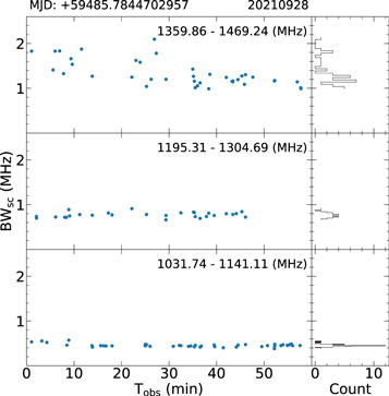
Figure 11. Scintillation bandwidth BWsc derived from some strong single bursts of FRB 20201124A on 2021 September 28 in three sub-bands plotted against the observation time Tobs. Their distributions are shown in the right sub-panels.
Download figure:
Standard image High-resolution imageTo get a clear relation between scintillation bandwidths and the observing frequencies, we integrated the energy of all bursts for each frequency channels, and then analyzed scintillation in a car-box sub-band of 1/4 band. The results are shown in Figure 12 for the center frequency ν and scintillation bandwidth BWsc, which can be fitted by a power-law function νs = a νγ , where γ = 3.0 is the power-law index.

Figure 12. Scintillation bandwidth of the integrated burst-energy spectrum of FRB 20201124A plotted against the central frequency of a car-box sub-band for scintillation calculation. The red dotted line denotes the power-law fitting.
Download figure:
Standard image High-resolution image
The scintillation bandwidth increases from about 0.5 MHz at 1.05 GHz to 1.4 MHz at 1.45 GHz in our observation frequency, with a mean scintillation bandwidth of about 0.94 MHz. The power-law index γ = 3.0 ± 0.2 is smaller than the value of 3.5 ± 0.01 obtained by Main et al. (2022), or 4.9 reported by Xu et al. (2022), or the theoretical value of 4.0 or 4.4 of Kolmogorov spectrum. The corresponding scattering timescale of about 0.31 μs is consistent with the results of Main et al. (2022), which is much smaller than the sampling time of 49.152 μs of our observation. Therefore scattering has an almost negligible effect on the morphological study for the bursts of FRB 20201124A. For the large number of bursts we observed, the properties shown in this paper should be intrinsic to the FRB 20201124A source.
We emphasize at the end of this paper that the sensitive observations by a large radio telescope such as the FAST is very important to detect rich features of bursts and reveal their properties. The classification scheme and other results presented in this paper are hard to be achieved without such sensitive observations. We also realize that multi-epoch wide-band observations are fundamental to understand the environment and physical mechanisms of FRB emission.
Acknowledgments
We thank the referee for helpful comments. This work makes use of the data from the FRB key science project, as one of five key projects of FAST, a Chinese national mega-science facility, operated by National Astronomical Observatories, Chinese Academy of Sciences. J. L. Han is supported by the National Natural Science Foundation of China (NSFC, Nos. 11988101 and 11833009) and the Key Research Program of the Chinese Academy of Sciences (Grant No. QYZDJ-SSW-SLH021). D. J. Zhou is supported by the Cultivation Project for the FAST scientific Payoff and Research Achievement of CAMS-CAS. Y. Feng is supported by the Key Research Project of Zhejiang Lab no. 2021PE0AC0. J. C. Jiang, K. J. Lee, H. Xu, C. F. Zhang, B. J. Wang, J. W. Xu are supported by the National SKA Program of China (2020SKA0120100), the National Key R&D Program of China (2017YFA0402602), the National Natural Science Foundation of China (No. 12041303), the CAS-MPG LEGACY project, and funding from the Max-Planck Partner Group.
Authors Contributions
D. J. Zhou developed the single pulse module and the related software for this work, and processed almost all data presented in this paper. J. L. Han realized the diversity on radio emission morphology on this special FRB source observed by the FAST, and led the writing of this paper. B. Zhang and W. W. Zhu proposed and chaired the FAST FRB key science project. B. Zhang, W. W. Zhu, J. L. Han, K. J. Lee and D. Li coordinated the teamwork, the observational campaign, co-supervised data analyses and interpretations. W. C. Jing analyzed the burst and sub-bursts parameter distributions. W.-Y. Wang performed the sub-pulse frequency analysis. Y. K. Zhang performed the analysis of energy distribution and the results are presented in Paper II of this series. J. C, Jiang performed the analysis of the polarization properties and the results are presented in Paper III. J. R. Niu performed the periodicity search and the results are presented in Paper IV. R. Luo improved the energy distribution analysis and make many suggestions to improve the paper. H. Xu, C. F. Zhang, B. J. Zhang, J. W. Xu, P. Wang, Z. L. Yang and Y. Feng also performed the single-pulse search, DM search, and the analysis of the burst energy, polarization, and periodicity search. All authors contributed to discussions and the paper writing.
Data Availability
Original FAST observation data can be accessible one year after observations. All data for the plots in this paper, including these in Appendix, can be obtained from the authors with a kind request.
Appendix: A Complete List of Detected Bursts of FRB 20201124A in 2021 September
In the FAST monitor sessions of 20210925-20210928, we detected 30, 62, 208, and 447 bursts in these 4 days, respectively. In total, there are 747 bursts. For each burst and the associated sub-bursts, the TOA expressed in MJD, the frequency of emission peak (ν0, in MHz), the detected emit low and high frequency (νlow and νhigh respectively, in MHz), the bandwidth (BWe, in MHz) of observed emission, the sub-burst width (Wsb, in ms), the detection signal-to-noise ratio (S/N), and the fluence (Fν , in mJy ms) together with the burst morphology classification, are all listed in Table A1 (available online as supplementary material).
We present the water-fall plot and burst profile for each burst, together with the energy distribution and the Gaussian fitting over the observational frequency. According to their morphology classification, the bursts can be found in Figures A1–A16 (available online as supplementary material at stacks.iop.org/RAA/22/124001/mmedia).
Footnotes
- 9
- 10
- 11
Supplementary data (44 MB, PDF) Table A1 and Figures A1–A16.