
Abstract
In this work, we study the magnetic field morphology of selected star-forming clouds spread over the galactic latitude (b) range −10° to 10°. The polarimetric observations of clouds CB24, CB27 and CB188 are conducted to study the magnetic field geometry of those clouds using the 104 cm Sampurnanand Telescope (ST) located at ARIES, Manora Peak, Nainital, India. These observations are combined with those of 14 further low latitude clouds available in the literature. Most of these clouds are located within a distance range 140–500 pc except for CB3 (∼2500 pc), CB34 (∼1500 pc), CB39 (∼1500 pc) and CB60 (∼1500 pc). Analyzing the polarimetric data of 17 clouds, we find that the alignment between the envelope magnetic field () and galactic plane (GP) (θGP) of the low-latitude clouds varies with their galactic longitudes (l). We observe a strong correlation between the longitude (l) and the offset () which shows that is parallel to the GP when the clouds are situated in the region 115° < l < 250°. However, has its own local deflection irrespective of the orientation of θGP when the clouds are at l < 100° and l > 250°. To check the consistency of our results, the stellar polarization data available in the Heiles catalog are overlaid on the DSS image of the clouds having mean polarization vector of field stars. The results are almost consistent with the Heiles data. A systematic discussion is presented in the paper. The effect of turbulence in the cloud is also studied which may play an important role in causing the misalignment phenomenon observed between and θGP. We have used Herschel (Herschel is an ESA space observatory with science instruments provided by European-led Principal Investigator consortia and with important participation from NASA.) SPIRE 500 μm and SCUBA 850 μm dust continuum emission maps in our work to understand the density structure of the clouds.


1. Introduction
Magnetic fields are present everywhere in our Galaxy, spreading the interstellar medium and expanding beyond the galactic disk. They are present in a broad variety of astrophysical objects, such as molecular clouds, pulsars and supernova remnants (Lu et al. 2020). Various astronomers extensively studied the large-scale galactic magnetic field (GMF), yet it remains inadequately understood. The GMF plays an essential role in forming molecular clouds that serve as the stellar nest in our Galaxy. Galactic fields could be sufficiently strong to inflict their direction upon individual molecular clouds (Shetty & Ostriker 2006), which can modulate the accumulation and fragmentation of the cloud (Li et al. 2011), thereby altering the efficiency of star formation (Price & Bate 2008). The magnetic field in molecular clouds plays a significant role in star formation efficiency (Hennebelle & Inutsuka 2019). Magnetic fields are also believed to have a considerable impact on the circumstellar disk formation as well as on fragmentation in forming binary systems (Price & Bate 2007). There are various other parameters responsible for star formation processes that involve turbulence (Li et al. 2004; Tilley & Pudritz 2004; Vázquez-Semadeni et al. 2005), jets and feedback from outflows (Li & Nakamura 2006; Pudritz & Ray 2019; Vázquez-Semadeni et al. 2019), and radiation feedback from the stars themselves (Clark et al. 2005). There is evidence of molecular clouds showing turbulent motions (Larson 1981; Mac Low & Klessen 2004). The impact of turbulence on the magnetic field structure is generally tough to interpret. However, some studies show that the magnetic field may play a dominant role in shaping the dynamics of the turbulence (Padoan & Nordlund 2002; Padoan et al. 2007, 2014). Thus, it is important to study the magnetic field morphology to understand the ongoing activities in molecular clouds.
When the background starlight passes through the aligned dust grains present in the interstellar medium, it gets polarized and the polarization position angle gives the orientation of the local magnetic field. Draine & Weingartner (1996) suggested that such alignment of the dust grains present in the molecular clouds may be due to the effect of radiative torque. The radiative torque mechanism is established on the interaction between radiation and grain to spin it up. The confirmation of radiative torque alignment (RAT) was established by Whittet et al. (2001) while studying the dense and diffuse gas in the Taurus cloud. In recent years, diverse studies were made on grain alignment by the RAT mechanism, which revealed that RAT happens to be a successful mechanism for alignment that can explain the dust grain alignment of numerous astrophysical environments (Hoang & Lazarian 2014; Andersson et al. 2015; Hoang et al. 2015). Hoang & Lazarian (2014) found that the linear polarization of nearby stars as predicted by the radiative alignment torque agrees well with the observational data, which demonstrates that polarization increases with the distance to the stars. Andersson et al. (2015) mentioned that the theory of interstellar grain alignment by RAT allows deriving specific, testable predictions for practical interstellar processes. Further detailed analysis of the RAT mechanism might give a promising explanation of grain alignment and polarimetry on the interstellar magnetic field and provide advanced information on dust characteristics.
Several researchers studied the orientation of the magnetic field through imaging polarimetry (Chakraborty et al. 2014; Soam et al. 2015, 2017; Chakraborty & Das 2016; Das et al. 2016; Jorquera & Bertrang 2018; Choudhury et al. 2019; Zielinski et al. 2021) and discussed the relative orientation of the magnetic field to the galactic plane (GP), outflow direction and minor axis of the cloud. The optical polarimetric analysis reveals that the envelope magnetic field of CB130 is oriented at an angle of 53° with respect to the orientation of GP (Chakraborty & Das 2016). Das et al. (2016) estimated the magnetic field strength of two submillimeter (sub-mm) cores of CB34 from the archival sub-mm polarimetric data. They presented the relative orientation of the envelope magnetic field with the minor axis of the cloud for both the cores, which supports magnetically dominated star formation models. Analyzing both optical and sub-mm polarimetric data of Bok globule CB17, Choudhury et al. (2019) reported a parallel alignment between the envelope magnetic field and the position angle of GP in contrast to the core-scale magnetic field, which is almost perpendicular to the GP. They also reported a relative orientation envelope magnetic field to the outflow axis and the cloud minor axis. Zielinski et al. (2021) discussed the magnetic field of a prototypical cloud B335 and observed a decrease in polarization toward the center of the cloud (dense core). They also observed a uniform pattern in the polarization vectors.
In this article, we present the magnetic field morphology of 17 star-forming clouds (including newly observed clouds CB24, CB27 and CB188), spread over the low galactic latitude range of −10° < b < 10°. Most of these clouds are located within a distance range 140–500 pc except for CB3 (2500 pc), CB34 (1500 pc), CB39 (1500 pc) and CB60 (1500 pc). We systematically study the alignment mechanism between the envelope magnetic field of the cloud and GP and their variation with galactic longitude. In Section 2 we describe the sources. In Section 3, we present the observations, data reduction procedures along with details on the archival data. In Section 4, we discuss the geometry of the envelope magnetic field of the three observed clouds. We summarize our results in Section 5.
2. Description of Sources
2.1. CB24
CB24 is a starless, small spherical cloud at a distance of 293 ± 54 pc (Das et al. 2015). There was no association with an IRAS point source identified. Kane et al. (1994) found that CB24 is a relatively less dense cloud, and the low column density may indicate that Bok globules like CB24 did not undergo significant core contraction and represent an ideal sample of starless small dark clouds.
2.2. CB27
CB27, also known as L1512, is an isolated Taurus core cloud near the GP. The distance of CB27 is found to be 140 pc (Kenyon et al. 1994). A compact sub-mm source (full width at half maximum, FWHM ∼ 104 au) is found to be present at the center of CB27 (Kirk et al. 2005; Di Francesco et al. 2008). The central density of the cloud is near to the maximum stable density, which is required for a pressure-supported, self gravitating cloud and this makes the cloud indistinguishable whether the core is a starless stable or a prestellar one (Launhardt et al. 2013).
2.3. CB188
CB188 is an isolated small cloud at a distance 262 ± 49 pc (Das et al. 2015). The bolometric luminosity of this cloud is 2.6 L⊙ and the envelope mass is about 0.7 M⊙ obtained from an interferometric study of the N2H+ (1–0) emission (Chen et al. 2007). The mean density of the core is ∼2 × 106 cm−3. CB188 is found to be physically associated with L673 (Tsitali et al. 2010), as shown by the dotted rectangle in the lower region of Figure 3. In our study, we only covered the northern region of the cloud CB188.
3. Observation, Data Reduction and Archival Data
3.1. Observations
We conducted the optical polarimetric observations of four fields toward the Bok globules CB27, CB24 and CB188 each on 2017 December 22, 23 and 2019 May 8, respectively. We have selected these three globules because of their close proximity with the GP (−10° < b < 10°) as we aim to study the magnetic field morphology of low latitude clouds. Also, no polarimetric study of these clouds was performed in the past. Moreover, the availability of dust continuum emission maps of CB27 (Herschel SPIRE 500 μm) and CB188 (and SCUBA 850 μm) also motivated us to select these globules. Polarimetric observations were conducted in the R-band (filter: λ = 630 nm, Δλ = 120 nm). The observed region around each globule is divided into four fields of 8' × 8' dimension because the CCD has a field of view of ∼8' in diameter. The observations were carried out with the 104 cm Sampurnanand Telescope (ST) at Aryabhatta Research Institute of Observational Sciences, Nainital, India (for exemplary previous polarimetric observations using this telescope see Chakraborty et al. 2014; Chakraborty & Das 2016; Das et al. 2016). The observation log is presented in Table 1. The 104 cm ST is an f/13 Cassegrain telescope. An Imaging Polarimeter (AIMPOL) is connected to the back-end of the telescope that has a Wollaston prism and a rotating half-wave plate (HWP). The Wollaston prism splits the incoming unpolarized light into two orthogonal components (ordinary and extraordinary), and the HWP rotates the polarization state of light into four angles 0°, 22 5, 45° and 675 which gives the four polarized components (see Das et al. 2013, for detailed observational procedures). The detailed theory and design of AIMPOL are presented in Rautela et al. (2004) and Medhi et al. (2008).
Table 1. Observation Log
| Object ID | Name of | Date | Field | R.A.(2000) | Decl.(2000) |
|---|---|---|---|---|---|
| Observatory | (h m s) | (° ' '') | |||
| CB24 | ARIES, Nainital | 2017 Dec 23 | F1 | 04:58:30 | 52:12:17 |
| F2 | 04:58:23 | 52:16:31 | |||
| F3 | 04:59:03 | 52:17:02 | |||
| F4 | 04:59:00 | 52:10:49 | |||
| CB27 | ARIES, Nainital | 2017 Dec 22 | F1 | 05:04:07 | 32:38:19 |
| F2 | 05:03:31 | 32:42:16 | |||
| F3 | 05:03:33 | 32:48:51 | |||
| F4 | 05:04:09 | 32:51:33 | |||
| CB188 | ARIES, Nainital | 2019 May 8 | F1 | 19:20:25 | 11:33:10 |
| F2 | 19:20:29 | 11:40:33 | |||
| F3 | 19:19:59 | 11:32:06 | |||
| F4 | 19:20:06 | 11:39:56 | |||
Download table as: ASCIITypeset image
3.2. Data Reduction: Imaging Polarimetry
We conducted the observation using the four rotations of HWP as mentioned in Section 3.1. For a particular rotation of HWP (α), the intensities (extraordinary, Ie and ordinary, Io ) of the two orthogonal polarized components are determined. If the HWP is rotated by α, the electric vector rotates by 2α. For calculation of the linear polarization it is useful to define the ratio Rα

where θ and p are the position angle and degree of linear polarization, respectively (Rautela et al. 2004). This ratio becomes Q/I and U/I when α = 0° and 225 respectively, i.e., the values of normalized Stokes parameters q and u (I: total intensity). The linear polarization (p) and the polarization position angle (θ) are given by

In principle, the linear polarization and the position angle of polarization can be measured from the first two rotations of HWP. However, the two additional rotations 45° and 675 are observed due to non-responsivity of the system.
The observed polarimetric data have been reduced using the Image Reduction and Analysis Facility (IRAF) package (see Rautela et al. 2004 for detailed data reduction procedures). The uncertainties associated with p and θ are calculated using the relations (Ramaprakash et al. 1998)

where N and Nb represent the flux counts corresponding to the source and background, respectively.
3.2.1. Instrumental Calibration
The instrumental calibration is determined by analyzing three low polarized standard stars HD 21447, γBoo and βUMa taken from Breeveld & Puchnarewicz (1998) and Schmidt et al. (1992) which are in sound agreement with the literature. The instrumental calibration for zero position angle of polarization is determined by analyzing four highly polarized standard stars HD 251204, HD 19820, HD 154445 and HD 161056 taken from Serkowski (1974) and Schmidt et al. (1992). The results obtained from our observations are presented in Table 2.
Table 2. Standard Star Polarimetry: Object ID, Date of Observation, Observed Values of p and θ, Literature Values of p and θ, and Reference
| Observed Value | Literature Value | ||||||
|---|---|---|---|---|---|---|---|
| Object ID | Date of Observation | p ± ep | θ ± eθ | p ± ep | θ ± eθ | Literature Reference | |
| (%) | (°) | (%) | (°) | ||||
| High polarized standard stars | |||||||
| HD 251204 | 2017 Dec 23 | 4.84 ± 0.17 | 154.3 ± 1.0 | 4.79 ± 0.30 | 155.7 | Serkowski (1974) | |
| HD 19820 | 2017 Dec 23 | 4.83 ± 0.18 | 115.4 ± 1.0 | 4.53 ± 0.03 | 114.5 ± 0.2 | Schmidt et al. (1992) | |
| HD 154445 | 2019 May 8 | 3.48 ± 0.09 | 89.7 ± 0.7 | 3.78 ± 0.06 | 88.8 ± 0.5 | Schmidt et al. (1992) | |
| HD 161056 | 2019 May 8 | 3.85 ± 0.10 | 69.5 ± 0.7 | 4.03 ± 0.03 | 66.9 ± 0.2 | Schmidt et al. (1992) | |
| Unpolarized standard stars | |||||||
| HD 21447 | 2017 Dec 23 | 0.11 ± 0.18 | 111.7 | 0.06 ± 0.03 | 110 | Breeveld & Puchnarewicz (1998) | |
| γBoo | 2019 May 8 | 0.19 ± 0.12 | 23.1 | 0.065 ± 0.02 | 21.3 | Schmidt et al. (1992) | |
| βUMa | 2019 May 8 | 0.10 ± 0.14 | 109.2 | 0.009 ± 0.02 | 107.8 | Schmidt et al. (1992) | |
Download table as: ASCIITypeset image
3.3. Archival Data
Our observed clouds are situated at low galactic latitude close to GP, which allows us to map the magnetic field morphology of the star-forming clouds near the GP. We collected 14 additional low galactic latitude star-forming clouds for which polarimetric observations at optical wavelength are available in literature allowing us to perform a systematic statistical analysis. These include 12 Bok globules (viz. CB3, CB4, CB17, CB25, CB26, CB34, CB39, CB56, CB60, CB69, CB130 and CB246) and two Lynd's clouds (viz. L1014 and L1415). All these clouds are located in the galactic latitude (b) range from −10° < b < 10°. Optical polarimetric observation of CB26 was performed by our group (P. Halder et al. 2022, in preparation). The details of the 17 clouds are compiled in Table 3.
Table 3. Details of Target Globules (Our Observation Along with Archival References of Polarimetric Studies)
| ID | R.A.(2000) | Decl.(2000) | l | b | Name of | Date of | Reference | Distance (ref) |
|---|---|---|---|---|---|---|---|---|
| (h m s) | (° ' '') | (°) | (°) | Observatory | Observation | (pc) | ||
| CB24 | 04 58 30 | +52 15 41 | 155.76 | 5.90 | a ST | 2017 Dec 23 | 293 ± 54 (1) | |
| CB27 | 05 04 09 | +32 43 12 | 171.82 | −5.18 | ST | 2017 Dec 22 | Our observations | 140 (2) |
| CB188 | 19 20 17 | +11 36 12 | 46.53 | −1.01 | ST | 2019 May 8 | 262 ± 49 (1) | |
| Archival Data | ||||||||
| CB3 | 00 28 45 | +56 42 08 | 119.80 | −6.03 | b MA | 1997 Dec 23 | Sen et al. (2000) | 2500 (3) |
| CB4 | 00 39 03 | +52 51 29 | 121.03 | −9.96 | c MB | 1986 Dec | Kane et al. (1995) | 350 ± 150 (4) |
| CB17 | 04 04 37 | +56 56 41 | 147.02 | 3.39 | ST | 2016 Mar 9 | Choudhury et al. (2019) | 253 ± 43 (5) |
| CB25 | 04 59 04 | +52 03 24 | 155.97 | 5.84 | MA | 1997 Dec 23 | Sen et al. (2000) | ⋯ |
| CB26 | 05 00 09 | +52 05 00 | 156.05 | 5.99 | ST | 2016 Dec 29 and 30 | P. Halder et al. (2022, in preparation) | 140 ± 20 (6) |
| CB34 | 05 47 02 | +21 00 10 | 186.94 | −3.83 | ST | 2013 Mar 12-13 | Das et al. (2016) | 1500 (3) |
| CB39 | 06 01 58 | +16 30 26 | 192.63 | −3.04 | MA | 1997 Dec 25 | Sen et al. (2000) | 1500 (3) |
| CB56 | 07 14 36 | −25 08 54 | 237.90 | −6.45 | IGO | 2011 Mar 4 | Chakraborty et al. (2014) | ⋯ |
| CB60 | 08 04 36 | −31 30 47 | 248.89 | −0.01 | d IGO | 2011 Mar 5 | Chakraborty et al. (2014) | 1500 (3) |
| CB69 | 17 02 42 | −33 17 00 | 351.23 | 5.14 | IGO | 2011 Mar 5 | Chakraborty et al. (2014) | 500 (3) |
| CB130 | 18 16 16 | −02 33 01 | 26.61 | 6.65 | IGO | 2014 Apr 26, 28 & 30 | Chakraborty & Das (2016) | 250 ± 50 (3) |
| 2014 May 2–4 | ||||||||
| CB246 | 23 56 44 | +58 34 29 | 115.84 | −3.54 | MA | 1997 Dec 24 | Sen et al. (2000) | 140 (3) |
| L1014 | 21 24 07 | +49 59 05 | 92.45 | −0.12 | ST | 2010 Nov 14 | Soam et al. (2015) | 258 ± 50 (7) |
| 2011 Nov 22 | ||||||||
| L1415 | 04 42 00 | +54 26 00 | 152.41 | 5.27 | ST | 2011 Nov 23 | Soam et al. (2017) | 250 (8) |
| 2011 Dec 19, 20 & 24 | ||||||||
| 2013 Oct 29 | ||||||||
Notes. Cloud ID, right ascension (R.A.), declination (Decl.), galactic longitude (l), galactic latitude (b), name of observatory, date of observation, reference and distance to the cloud (d).
a ST: Sampurnanand Telescope, ARIES, Nainital. b MA: Mount Abu, India. c MB: Mount Bigelow, North of Tucson, Arizona. d IGO: IUCAA Girawali Observatory, Pune.Distance References: (1) Das et al. (2015). (2) Kenyon et al. (1994). (3) Launhardt & Henning (1997). (4) Perrot & Grenier (2003). (5) Choudhury et al. (2019). (6) Launhardt et al. (2010). (7) Soam et al. (2015). (8) Soam et al. (2017).
Download table as: ASCIITypeset image
4. Geometry of Envelope Magnetic Field
We reduce the optical polarimetric data of CB24, CB27 and CB188 using IRAF (as discussed in Section 3.2). The values of θ and p of the background stars detected toward the field of the three clouds are calculated using Equation (2). We consider only those sources with p/ep ≥ 3 (here ep denotes the polarization error). To avoid the foreground polarization, we make use of Gaia Early Data Release 3 (EDR3) parallaxes (Gaia Collaboration et al. 2016, 2021) to determine the distance of the individual field stars toward each cloud. The critical distance is set to be the distance of the respective cloud (293 ± 54 pc for CB24, 140 pc for CB27 and 262 ± 49 pc for CB188). For further analysis, we consider only sources with distances beyond the critical distance. In the case of CB24, polarization measurements of 20 fields stars are found, out of which three sources (#7, #12 and #14) have been identified to be foreground to the cloud. Moreover, Gaia parallaxes for two sources (#11 and #13) are not available, so we discarded these five sources from further analysis. In the case of CB27, polarization measurements of 27 field stars are found, 26 of which have been identified to be background to the cloud while one source (#16) does not have a Gaia parallax available and hence we discard this star from the analysis as well. However, in the case of CB188, polarization measurements of 24 field stars are found and all these 24 sources have been identified to be background to the cloud.
Fifteen field stars are detected toward CB24, twenty-six field stars toward CB27 and twenty-four field stars are detected in the field of CB188. The values of p and θ with the uncertainties of the field stars toward these three clouds are presented in Tables 4–6, respectively. The mean values of degree of polarization (〈p〉) along with the standard error 5 are estimated to be (2.67 ± 0.27)% for CB24, (2.10 ± 0.19)% for CB27 and (3.11 ± 0.28)% for CB188. The mean orientations of polarization position angle (〈θ〉) with the standard error are estimated to be (142.8 ± 5.7)° for CB24, (145.5 ± 3.7)° for CB27 and (98.5 ± 2.3)° for CB188.
Table 4. Polarimetric Results of 20 Field Stars Toward CB24
| Star ID | R.A.(2000) | Decl.(2000) | p ± ep | θ ± eθ | d ± ed | Background Star |
|---|---|---|---|---|---|---|
| (h m s) | (° ' '') | (%) | (°) | (pc) | (yes/no) | |
| 1 | 4 59 17.76 | 52 08 31 | 3.85 ± 0.46 | 146.8 ± 3.4 | 1739 ± 70 | yes |
| 2 | 4 59 12.72 | 52 07 33 | 1.99 ± 0.29 | 86.0 ± 4.2 | 726 ± 8 | yes |
| 3 | 4 59 11.28 | 52 08 09 | 1.66 ± 0.49 | 98.3 ± 8.4 | 700 ± 10 | yes |
| 4 | 4 59 11.04 | 52 17 34 | 1.52 ± 0.39 | 158.5 ± 7.3 | 643 ± 7 | yes |
| 5 | 4 59 06.24 | 52 18 21 | 2.31 ± 0.40 | 161.5 ± 4.9 | 361 ± 2 | yes |
| 6 | 4 59 03.36 | 52 08 09 | 2.38 ± 0.54 | 143.4 ± 6.5 | 3702 ± 307 | yes |
| 7 | 4 58 59.76 | 52 19 15 | 1.91 ± 0.20 | 159.9 ± 3.0 | 297 ± 2 | no |
| 8 | 4 58 48.72 | 52 20 20 | 1.39 ± 0.39 | 145.8 ± 8.0 | 817 ± 38 | yes |
| 9 | 4 58 47.28 | 52 12 43 | 2.24 ± 0.74 | 137.5 ± 9.5 | 2330 ± 164 | yes |
| 10 | 4 58 34.80 | 52 19 33 | 2.00 ± 0.35 | 159.5 ± 5.0 | 501 ± 14 | yes |
| 11 | 4 58 32.16 | 52 18 18 | 3.54 ± 0.62 | 150.0 ± 5.0 | NA | ⋯ |
| 12 | 4 58 27.60 | 52 17 13 | 2.03 ± 0.25 | 169.1 ± 3.6 | 324 ± 1 | no |
| 13 | 4 58 23.28 | 52 09 39 | 1.22 ± 0.21 | 125.4 ± 4.8 | NA | ⋯ |
| 14 | 4 58 22.80 | 52 16 37 | 1.76 ± 0.47 | 162.1 ± 7.6 | 334 ± 2 | no |
| 15 | 4 58 21.12 | 52 17 34 | 3.85 ± 0.66 | 147.1 ± 4.9 | 3891 ± 269 | yes |
| 16 | 4 58 18.24 | 52 17 45 | 1.58 ± 0.29 | 153.6 ± 5.3 | 617 ± 6 | yes |
| 17 | 4 58 12.00 | 52 11 24 | 3.24 ± 0.35 | 165.0 ± 3.1 | 510 ± 4 | yes |
| 18 | 4 58 10.32 | 52 16 15 | 4.01 ± 0.35 | 143.5 ± 2.5 | 3165 ± 226 | yes |
| 19 | 4 58 09.36 | 52 18 43 | 3.89 ± 1.14 | 145.8 ± 8.4 | 3942 ± 486 | yes |
| 20 | 4 58 06.48 | 52 18 36 | 4.13 ± 0.84 | 149.7 ± 5.8 | 4498 ± 1354 | yes |
Note. The R.A. and decl. of the field stars are given in columns 2 and 3 respectively, columns 4 and 5 represent the degree of linear polarization (p) and position angle of polarization (θ) respectively, and column 6 gives the distance (d in pc) to the individual field stars collected from the Gaia EDR3 database. A star having distance more than the distance of the cloud CB24 (∼360 pc) is considered to be background to the cloud and is listed in column 7.
Download table as: ASCIITypeset image
Table 5. Polarimetric Results of 27 Field Stars in CB27
| Star ID | R.A.(2000) | Decl.(2000) | p ± ep | θ ± eθ | d ± ed | Background Star |
|---|---|---|---|---|---|---|
| (h m s) | (° ' '') | (%) | (°) | (pc) | (yes/no) | |
| 1 | 05 04 24.72 | 32 54 10 | 0.64 ± 0.19 | 139.8 ± 8.6 | 1255 ± 38 | yes |
| 2 | 05 04 24.48 | 32 51 46 | 1.58 ± 0.22 | 103.0 ± 4.0 | 316 ± 5 | yes |
| 3 | 05 04 18.48 | 32 52 44 | 1.20 ± 0.34 | 159.5 ± 8.1 | 937 ± 15 | yes |
| 4 | 05 04 16.32 | 32 40 04 | 0.93 ± 0.21 | 147.0 ± 6.4 | 2829 ± 168 | yes |
| 5 | 05 04 16.08 | 32 38 31 | 1.20 ± 0.31 | 83.1 ± 7.3 | 2266 ± 406 | yes |
| 6 | 05 04 14.40 | 32 38 16 | 1.14 ± 0.25 | 159.5 ± 6.4 | 1337 ± 30 | yes |
| 7 | 05 04 11.28 | 32 35 34 | 0.89 ± 0.21 | 150.0 ± 6.9 | 1409 ± 35 | yes |
| 8 | 05 04 07.92 | 32 49 37 | 2.96 ± 0.57 | 165.1 ± 5.5 | 2286 ± 184 | yes |
| 9 | 05 03 58.32 | 32 41 16 | 1.51 ± 0.28 | 123.9 ± 5.4 | 1293 ± 28 | yes |
| 10 | 05 03 53.76 | 32 54 14 | 2.18 ± 0.22 | 146.7 ± 2.9 | 1364 ± 32 | yes |
| 11 | 05 03 50.64 | 32 50 42 | 1.76 ± 0.47 | 158.4 ± 7.6 | 363 ± 2 | yes |
| 12 | 05 03 48.24 | 32 51 14 | 5.20 ± 1.10 | 149.9 ± 6.0 | 1829 ± 117 | yes |
| 13 | 05 03 47.04 | 32 40 22 | 3.18 ± 0.35 | 135.4 ± 3.1 | 766 ± 18 | yes |
| 14 | 05 03 42.24 | 32 47 02 | 2.43 ± 0.30 | 158.5 ± 3.5 | 1526 ± 63 | yes |
| 15 | 05 03 42.00 | 32 46 01 | 1.56 ± 0.28 | 159.3 ± 5.1 | 424 ± 3 | yes |
| 16 | 05 03 39.84 | 32 48 10 | 2.76 ± 0.68 | 142.0 ± 7.0 | NA | ⋯ |
| 17 | 05 03 39.60 | 32 45 46 | 1.59 ± 0.29 | 157.2 ± 5.2 | 1077 ± 19 | yes |
| 18 | 05 03 38.88 | 32 50 06 | 2.83 ± 0.49 | 148.8 ± 4.9 | 2826 ± 166 | yes |
| 19 | 05 03 34.32 | 32 38 27 | 2.61 ± 0.37 | 129.8 ± 4.1 | 5155 ± 492 | yes |
| 20 | 05 03 30.48 | 32 51 46 | 2.45 ± 0.58 | 157.4 ± 6.8 | 655 ± 9 | yes |
| 21 | 05 03 28.56 | 32 49 33 | 2.84 ± 0.72 | 147.5 ± 7.2 | 5176 ± 721 | yes |
| 22 | 05 03 24.00 | 32 50 45 | 2.97 ± 0.75 | 150.8 ± 7.3 | 5288 ± 590 | yes |
| 23 | 05 03 23.52 | 32 48 54 | 2.82 ± 0.34 | 150.7 ± 3.4 | 1860 ± 93 | yes |
| 24 | 05 03 22.32 | 32 52 04 | 2.72 ± 0.35 | 148.3 ± 3.7 | 644 ± 10 | yes |
| 25 | 05 03 21.12 | 32 48 39 | 2.10 ± 0.27 | 153.1 ± 3.7 | 710 ± 13 | yes |
| 26 | 05 03 17.04 | 32 43 08 | 1.33 ± 0.24 | 135.6 ± 5.1 | 1586 ± 69 | yes |
| 27 | 05 03 16.32 | 32 45 43 | 1.92 ± 0.21 | 165.4 ± 3.1 | 711 ± 9 | yes |
Note. The R.A. and decl. of the field stars are given in columns 2 and 3 respectively, columns 4 and 5 represent p and θ respectively and column 6 gives the distance (d in pc) to the individual field stars collected from the Gaia EDR3 database. A star having distance more than the distance of the cloud CB24 (∼140 pc) is considered to be background to the cloud and is listed in column 7.
Download table as: ASCIITypeset image
Table 6. Polarimetric Results of 24 Field Stars in CB188
| Star ID | R.A.(2000) | Decl.(2000) | p ± ep | θ ± eθ | d ± ed | Background Star |
|---|---|---|---|---|---|---|
| (h m s) | (° ' '') | (%) | (°) | (pc) | (yes/no) | |
| 1 | 19 20 43.57 | 11 39 34 | 3.30 ± 1.02 | 100.0 ± 8.9 | 2919 ± 167 | yes |
| 2 | 19 20 40.52 | 11 41 50 | 4.53 ± 1.16 | 96.3 ± 7.4 | 2520 ± 164 | yes |
| 3 | 19 20 40.15 | 11 41 47 | 4.30 ± 1.18 | 96.9 ± 7.9 | 2229 ± 136 | yes |
| 4 | 19 20 38.12 | 11 42 59 | 3.04 ± 1.01 | 126.6 ± 9.5 | 666 ± 8 | yes |
| 5 | 19 20 34.64 | 11 41 31 | 2.40 ± 0.39 | 86.1 ± 4.6 | 1166 ± 17 | yes |
| 6 | 19 20 31.70 | 11 41 07 | 3.81 ± 1.22 | 105.5 ± 9.2 | 2704 ± 184 | yes |
| 7 | 19 20 30.77 | 11 38 37 | 3.42 ± 0.68 | 90.4 ± 5.7 | 2498 ± 166 | yes |
| 8 | 19 20 30.43 | 11 40 10 | 4.13 ± 1.29 | 89.6 ± 8.9 | 1448 ± 46 | yes |
| 9 | 19 20 28.00 | 11 43 59 | 2.82 ± 0.40 | 93.3 ± 4.1 | 1016 ± 18 | yes |
| 10 | 19 20 24.52 | 11 43 45 | 5.14 ± 1.45 | 97.8 ± 8.1 | 1462 ± 50 | yes |
| 11 | 19 20 23.11 | 11 38 35 | 1.54 ± 0.51 | 93.9 ± 9.5 | 394 ± 3 | yes |
| 12 | 19 20 22.20 | 11 42 48 | 4.29 ± 1.21 | 88.8 ± 8.1 | 1453 ± 56 | yes |
| 13 | 19 20 21.95 | 11 34 15 | 1.69 ± 0.47 | 119.5 ± 7.9 | 2661 ± 214 | yes |
| 14 | 19 20 16.00 | 11 41 30 | 5.82 ± 0.37 | 96.8 ± 1.8 | 2938 ± 298 | yes |
| 15 | 19 20 15.34 | 11 40 53 | 1.68 ± 0.53 | 92.5 ± 9.0 | 857 ± 11 | yes |
| 16 | 19 20 12.79 | 11 39 01 | 2.94 ± 0.98 | 99.4 ± 9.5 | 929 ± 33 | yes |
| 17 | 19 20 10.97 | 11 42 05 | 1.83 ± 0.61 | 90.4 ± 9.6 | 903 ± 15 | yes |
| 18 | 19 20 07.00 | 11 36 13 | 2.81 ± 0.93 | 116.4 ± 9.5 | 717 ± 18 | yes |
| 19 | 19 20 05.72 | 11 31 45 | 1.24 ± 0.41 | 95.3 ± 9.5 | 869 ± 13 | yes |
| 20 | 19 20 02.06 | 11 36 11 | 1.89 ± 0.32 | 82.0 ± 4.9 | 1072 ± 22 | yes |
| 21 | 19 20 01.69 | 11 42 57 | 1.58 ± 0.52 | 88.3 ± 9.4 | 838 ± 12 | yes |
| 22 | 19 19 59.76 | 11 31 36 | 1.65 ± 0.55 | 97.1 ± 9.5 | 838 ± 11 | yes |
| 23 | 19 19 59.64 | 11 39 52 | 4.80 ± 1.51 | 112.7 ± 9.0 | 2479 ± 189 | yes |
| 24 | 19 19 56.55 | 11 41 02 | 4.01 ± 1.01 | 108.5 ± 7.1 | 1063 ± 25 | yes |
Note. The R.A. and decl. of the field stars are given in columns 2 and 3 respectively, columns 4 and 5 represent p and θ respectively and column 6 gives the distance (d in pc) to the individual field stars collected from the Gaia EDR3 database. The star having distance more than the distance of the cloud CB24 (∼300 pc) is considered to be background to the cloud and is listed in column 7.
Download table as: ASCIITypeset image
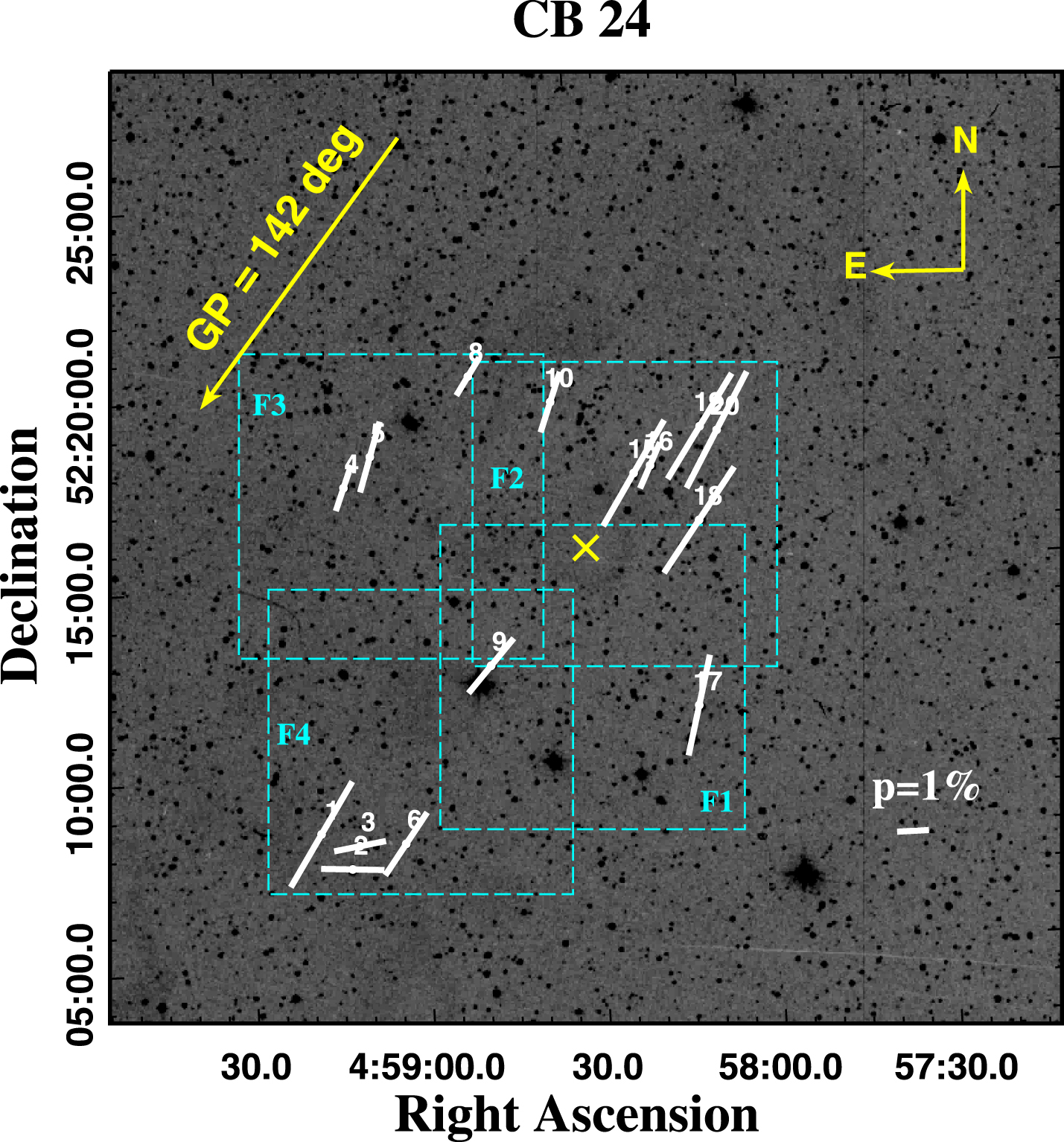
Using the values of p and θ, polarization maps are generated for the three clouds. The polarization vectors are plotted on a 25' × 25' Digitized Sky Survey (DSS) image of CB24, CB27 and CB188 and are presented in Figures 1–3, respectively. The solid lines represent the polarization vectors whose length corresponds to p, and the inclination is θ. The cross marks the center of the cloud. At the bottom right corner of each map, a vector of 1% polarization is drawn for reference. The vector at the top corner signifies the orientation of the GP (θGP), which is 142° for CB24, 1425 for CB27 and 28° for CB188. The mean value of the position angle of polarization 〈θ〉 represents the orientation of envelope magnetic field of the cloud, i.e., 〈θ〉 = . Also, on the polarization map of CB27 (Figure 2), the contours extracted from Herschel SPIRE 500 μm dust continuum emission map are plotted (magenta). The thermal dust continuum map is used to understand the density structure of the globule. In Figure 3, the SCUBA
6
850 μm dust continuum emissions is overlaid (magenta) on the polarization map of CB188. The region of cloud L673 which is physically associated with the field of CB188 as mentioned in Section 2.3 is also marked by the yellow dotted rectangle in Figure 3.


Figure 1. Polarization map of CB24: White solid lines represent the polarization vectors of the background field stars plotted on a DSS image of the globule CB24 (25' × 25'). At the bottom right corner, a vector of 1% polarization is shown for reference. The vector at the top left corner indicates the orientation of the GP (θGP = 142°). The center of the globule is marked by the cross. The dashed rectangular boxes of dimension 8' × 8' show the fields of observation (details are given in Table 1) of the cloud.
Download figure:
Standard image High-resolution image
Figure 2. Polarization map of CB27: White solid lines represent the polarization vectors of the background field stars plotted on a DSS image of the globule CB27 (25' × 25'). At the bottom right corner, a vector of 1% polarization is displayed for reference. The vector at the top left corner indicates the orientation of the GP (θGP = 1425). The cross marks the center of the globule. The dashed rectangular boxes of dimension 8' × 8' show the fields of observation (details are given in Table 1) of the cloud. Also, the contours extracted from the Herschel SPIRE 500 μm dust continuum emission map in the range of 18–74 mJy beam−1 with an increasing step size of 8 mJy beam−1 are plotted (magenta) over the polarization map.
Download figure:
Standard image High-resolution image
Figure 3. (a) Polarization map of CB188: White solid lines represent the polarization vectors of the background field stars plotted on a DSS image of the globule CB188 (25' × 25'). At the bottom right corner, a vector of 1% polarization is shown for reference. The vector at the top right corner indicates the orientation of the GP (θGP = 28°). The cross marks the center of the globule. The dashed rectangular boxes of dimension 8' × 8' show the fields of observation (details are given in Table 1) of the cloud. Also, the contours extracted from the SCUBA 850 μm dust continuum emission map in the range of 112–336 mJy beam−1 with an increasing step size of 54 mJy beam−1 are plotted (magenta) over the polarization map. The dotted rectangle in the lower region represents Lynd's cloud L673, which is physically associated with the field of CB188 (see Section 2 for details). (b) The zoomed-in view of the central region for a better view of the contours extracted from the SCUBA 850 μm dust continuum emission map is plotted over a 5' × 5' DSS image of the globule CB188.
Download figure:
Standard image High-resolution imageIt is evident from Figures 1 and 2 that the polarization vectors of all the field stars are more or less unidirectional and almost aligned along the GP. As can be further noticed from the contours overplotted on the polarization map of CB27 (Figure 2), the polarization vectors are oriented along the direction of the core (extracted from the SPIRE data). Also, there are two polarization vectors (#8 and #3) in the range of contours that show parallel orientation with the alignment of the core. The offset between the envelope magnetic field (given by the mean orientation of the polarization vectors) and the orientation of the GP, is 08 in CB24 and 29 in CB27. So, the envelope magnetic field orientation is clearly aligned along the GP in both the clouds. A similar trend was observed for cloud CB17 by Choudhury et al. (2019). In contrast, in the case of CB188, θoff = 705 (Figure 3) though all the polarization vectors are unidirectional. Also, the envelope magnetic field orientation is different from the alignment of the 850 μm dust emission contours. Thus, it can be inferred that the orientation of the envelope magnetic field in CB188 is not parallel with the GP, unlike CB24 and CB27. To build a basis for statistically relevant conclusions about the relative orientations of magnetic field traced in the envelope region of the globules with respect to the GP, we include polarimetric data of 14 further low galactic latitude (−10° < b < 10°) clouds from the literature. The corresponding results are summarized in Table 7.

Table 7. Parameters Related to the Target Globules Obtained from Our Study as well as from Literature: Cloud ID, Galactic Longitude (l), Galactic Latitude (b), Mean Value of Degree of Polarization (〈p〉), Position Angle of GP (θGP), Position Angle of Envelope Magnetic Field (), Offset (), FWHM (ΔV), Uncertainty Associated with ΔV and Position Angle of Core Magnetic Field ()


| ID | l | b | 〈p〉 | θGP ± | ± | θoff ± | ΔV ± eΔV | eΔV Associated | |
|---|---|---|---|---|---|---|---|---|---|
| (FWHM) | with ΔV are: | ||||||||
| (°) | (°) | (%) | (°) | (°) | (°) | (km s−1) | (°) | ||
| CB3 | 119.8 | −6.03 | 1.41 | 85.0 ± 0.03 | 65.4 ± 2.8 | 19.6 ± 2.8 | 1.60 ± 0.03 a | S.E. j | 69.0 f |
| CB4 | 121.03 | −9.96 | 2.84 | 87.2 ± 0.03 | 70.6 ± 2.9 | 16.7 ± 2.9 | 0.51 ± 0.01 c | S.E. | ⋯ |
| CB17 | 147.02 | 3.39 | 3.52 | 132.0 ± 0.04 | 136.0 ± 0.7 | 4.0 ± 0.7 | 0.97 ± 0.03 c | S.E. | 44.0 g |
| CB24 | 155.76 | 5.9 | 2.67 | 142.0 ± 0.04 | 142.8 ± 5.7 | 0.8 ± 5.7 | 0.80 ± 0.50 b | S.D. k | ⋯ |
| CB25 | 155.97 | 5.84 | 2.35 | 142.0 ± 0.04 | 150.9 ± 1.3 | 8.9 ± 1.3 | 0.70 ± 0.50 b | S.D. | ⋯ |
| CB26 | 156.05 | 5.99 | 3.00 | 142.0 ± 0.04 | 148.2 ± 1.0 | 6.2 ± 0.0 | 1.17 ± 0.02 c | S.E. | 25.3 h |
| CB27 | 171.82 | −5.18 | 2.10 | 142.6 ± 0.04 | 145.5 ± 3.7 | 2.9 ± 3.7 | 0.89 ± 0.01 c | S.E. | ⋯ |
| CB34 | 186.94 | −3.83 | 2.14 | 148.8 ± 0.04 | 143.3 ± 1.3 | 5.5 ± 1.3 | 1.50 ± 0.08 a | S.E. | 46.7 for Core1 i |
| 90.4 for Core2 i | |||||||||
| CB39 | 192.63 | −3.04 | 1.95 | 150.4 ± 0.03 | 150.3 ± 7.7 | 0.1 ± 7.7 | 2.05 ± 0.50 b | S.D. | ⋯ |
| CB56 | 237.9 | −6.45 | 1.08 | 152.3 ± 0.02 | 150.9 ± 2.4 | 1.4 ± 2.4 | 1.44 ± 0.50 b | S.D. | ⋯ |
| CB60 | 248.89 | −0.01 | 1.30 | 147.7 ± 0.01 | 155.2 ± 3.0 | 7.5 ± 3.0 | 1.82 ± 0.40 b | S.D. | ⋯ |
| CB69 | 351.23 | 5.14 | 2.00 | 37.7 ± 0.04 | 155.8 ± 3.3 | 118.1 ± 3.3 | 2.35 ± 0.50 b | S.D. | ⋯ |
| CB130 | 26.61 | 6.65 | 2.53 | 28.4 ± 0.03 | 80.0 ± 3.2 | 51.6 ± 3.2 | 4.20 c ± ⋯ | − | ⋯ |
| CB188 | 46.53 | −1.02 | 3.11 | 28.0 ± 0.01 | 98.5 ± 2.3 | 70.5 ± 2.3 | 4.40 ± 1.1 b | S.D. | ⋯ |
| CB246 | 115.84 | −3.54 | 1.92 | 77.9 ± 0.03 | 67.4 ± 5.2 | 10.5 ± 5.2 | 1.62 ± 0.50 b | S.D. | ⋯ |
| L1014 | 92.45 | −0.12 | 1.90 | 45.2 ± 0.02 | 15.0 ± 2.2 | 30.2 ± 2.2 | 2.26 ± 0.05 d | S.E. | ⋯ |
| L1415 | 152.41 | 5.27 | 3.10 | 138.0 ± 0.04 | 155.0 ± 0.7 | 17.0 ± 0.7 | 1.65 ± 0.02 e | S.E. | − |


Notes.
a Wang et al. (1995). b Clemens et al. (1991). c Lippok et al. (2013). d Crapsi et al. (2005). e Soam et al. (2017). f Ward-Thompson et al. (2009). g Choudhury et al. (2019). h Henning et al. (2001). i Das et al. (2016). j S.E.: Standard error of the mean. k S.D: Standard deviation.Download table as: ASCIITypeset image
5. Results and Discussion
In this section, we discuss the results of the presented polarization measurements. In Table 7, we present the angular offset in the orientation of envelope magnetic field (, traced through optical polarimetry) with the orientation of GP (θGP). The uncertainties in considered here are the standard error of the mean. Note that, due to the unavailability of the orientation of core-scale magnetic field () for the majority of the clouds, it is not possible to estimate the morphology of the core-magnetic field of the clouds. The interpretations based on the results obtained are discussed in the following subsections.


5.1. Relative Orientation between the Magnetic Field and the Galactic Plane
Various studies were carried out to find a correlation between the orientation of envelope magnetic field in molecular clouds with the orientation of the GP (e.g., Sen et al. 2000; Soam et al. 2015; Chakraborty & Das 2016; Das et al. 2016; Choudhury et al. 2019). The magnetic lines of force in the spiral arm of our Galaxy are parallel to the arm everywhere (Ireland & Hoyle 1961). In our previous work, the polarimetric study of CB17 reveals that the projected envelope magnetic field of the globule is oriented along the GP (Choudhury et al. 2019).
Based on the results of 17 clouds presented here, the mean value of position angle of polarization () determined for 13 clouds shows that the envelope magnetic field is almost aligned along the position angle of GP (θGP) (see Figure 4). The offset between the orientation of magnetic field and the GP (θoff) for these 13 clouds is within 20° with an average offset of 78. However, for four other clouds, a decoupling in the relative orientation between the magnetic field and the GP is observed with an average offset of 676. The details are listed in Table 7.


Figure 4. The variation of the alignment of envelope magnetic field of star-forming clouds along the GP, (along Y-axis) with their galactic longitude l (along X-axis) in case of low latitude clouds (−10° < b < 10°). "C" stands for CB cloud and "L" stands for Lynd's cloud. Also, note that the errors associated with are the standard error of the mean.


Download figure:
Standard image High-resolution image5.2. Variation in the Relative Orientation between the Magnetic Field and the GP with the Galactic Longitude
In this section, we discuss the possible correlation in the relative orientation between the magnetic field and the GP with the galactic longitude. In Figure 4, we show the variation in the offset between the orientation of envelope magnetic field and the GP, θoff (), with the galactic longitude (l). In this plot, we have considered only the magnitude of the offset and not the sign.

In our sample size, we have adequate data points in longitude range 0° to 250°. A second order polynomial fitting is done with these data points (solid curve) and a strong correlation is observed between l and θoff, with an equation, θoff = a1. l2 − b1. l + c1, where a1 = 0.0020 ± 0.0006, b1 = 0.8380 ± 0.1841 and c1 = 90.5358 ± 14.09. The fitting is done by including the error (standard error of the mean) in θoff. To test the goodness of fit, we estimated the coefficient of determination (R2) of the best fitted equation. R2 is a key output of regression analysis that may be interpreted as the proportion of the variance in the dependent variable predicted from the independent variable, which lies between 0 and 1. The higher the coefficient, the better is the goodness of fit. In this case, R2 is estimated to be ≈0.87. It is evident from this figure that the offset between the orientation of GP and the envelope magnetic field is relatively low in the region 115° < l < 250° (which corresponds to the region toward the galactic anti-center, GAC). This indicates that the local magnetic field of the clouds situated toward the GAC region is oriented along the GP. The significant offset between the and θGP observed in the region l < 100° (corresponding to the region toward the galactic center, GC) shows that the orientation of the magnetic field in the clouds lying in those regions (CB130, CB188 and L1014) tends to become perpendicular to the GP. Hence, for the clouds located at those longitudes, the envelope magnetic field has a local deflection of its own irrespective of the orientation of GP.

Note that no CB cloud is located in the region 250° < l < 350° in the molecular cloud catalog of Clemens & Barvainis (1988). However, since there is one single cloud (CB69) available between 350° and 360° which has a huge offset between the orientation of envelope magnetic field and GP, we have included this cloud in our sample size to observe the best fitting parameters. A second order polynomial fitting is done which is represented by the dashed curve. The curve appears to follow the same trend as in the region l < 100°, which indicates that, toward the GC region, the clouds possess their own local deflection irrespective of the orientation of GP. In this case, R2 is estimated to be ≈0.81 and the fitting equation is θoff = a2. l2 − b2. l + c2, where a2 = 0.0032 ± 0.0004, b2 = 1.1177 ± 0.1484 and c2 = 105.559 ± 13.82. Although we have made an attempt to fit the equation including CB69, the fitting parameters obtained may not be significant enough due to insufficient data points beyond l > 250°.
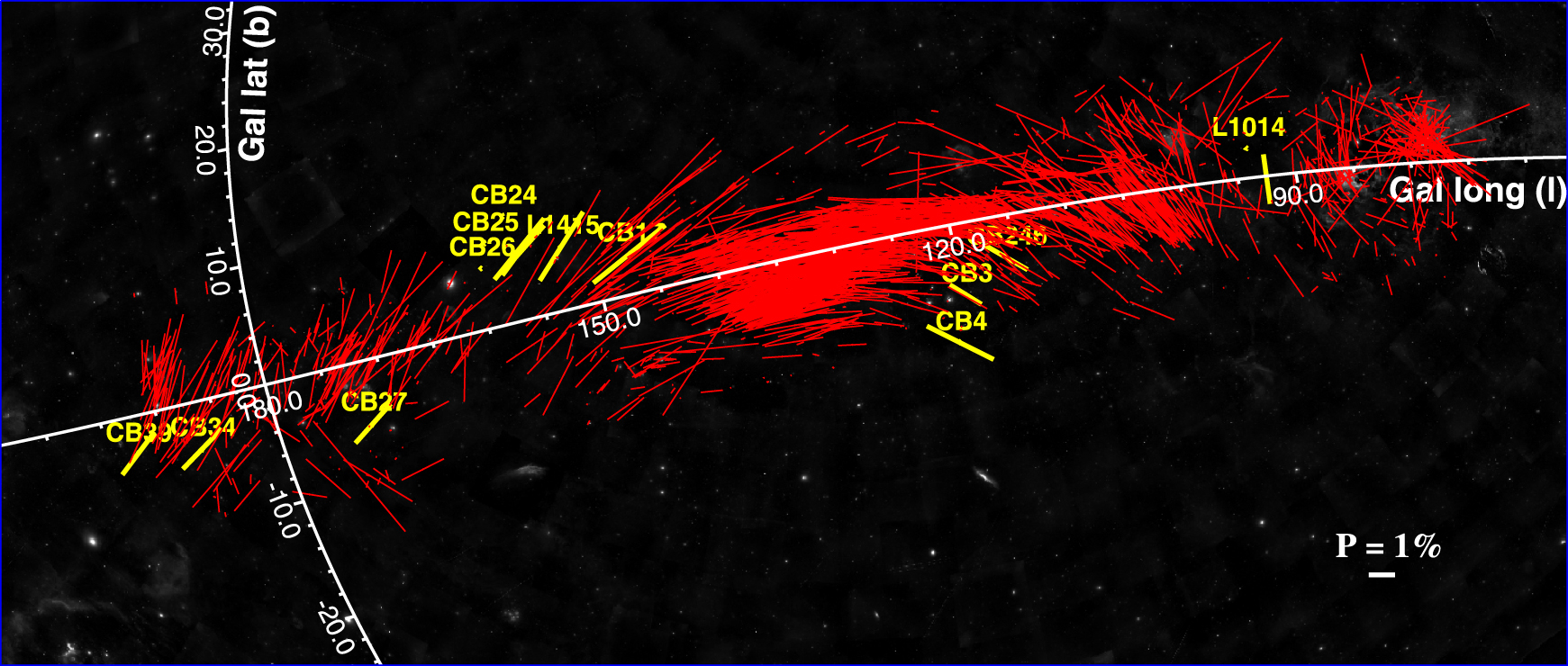
We compare the polarization of the clouds with the polarization of the stars by Heiles (2000) to interpret the relative orientation of the local magnetic field and the GP. The stellar polarization catalogs compiled by Heiles (2000) contain polarization data of 9268 stars in the whole sky (−90° < b < 90°) with p and θ ranging from 0% to 12.47% and 0°–180°. As the region of interest in our study is −10° < b < 10°, we have extracted 2386 polarization data of stars from the Heiles catalog within this range. In Figures 5–7, the mean degree of polarization (〈p〉) and position angle of polarization vectors (〈θ〉) of the field stars located in the clouds are overlaid along with the stellar polarization vectors obtained from the Heiles catalog on the DSS image. The red lines represent stellar polarization vectors obtained from the Heiles catalog and yellow lines signify the mean polarization vectors of the stars background to the clouds (indicated by the cloud IDs). In Table 8, we have presented the mean position angle of stellar polarization vectors (〈θHeiles〉) and the standard deviation () in the selected longitude range where the studied clouds are located. The polarization vectors of 1523 stars obtained from the Heiles catalog are plotted in Figure 5 along with 〈p〉 and 〈θ〉 of twelve clouds, viz., CB3, CB4, CB17, CB24, CB25, CB26, CB27, CB34, CB39, CB246, L1014 and L1415 in the longitude range 88° < l < 195°. In Figure 6, 156 stellar polarization vectors are plotted along with 〈p〉 and 〈θ〉 of CB56 and CB60, situated in the longitude range 235° < l < 250° that corresponds to the region of GAC. We have also presented polarization vectors of 724 stars along with 〈p〉 and 〈θ〉 of CB69, CB130, and CB188 situated in the longitude range l > 350° and l < 60° corresponding to the region of GC in Figure 7. Misalignment among stellar polarization vectors at particular longitude ranges is noted to be strong when < 2 (see Table 8). As revealed from Figure 5 and Table 8, the observed nine star-forming clouds in the longitude range 110° < l < 180° are found to be almost aligned with the stellar polarization vectors at their local regions which correspond to the region of GAC. A slight randomness is observed in the region 185° < l < 195° where CB34 and CB39 are located. However, in the region around l ∼ 90° toward GC , a significant randomness in the alignment of stellar polarization vectors is seen where the cloud L1014 is located. In Figure 6, almost unidirectional orientation of the stellar polarization vectors is observed in the region 235° < l < 250° . However, in Figure 7, misalignment in the orientation of stellar polarization vectors as well as the star-forming clouds is observed in the regions 345° < l < 355° and 20° < l < 50° . Thus, a local irregularity is observed toward GC as revealed from the stellar polarization data of Heiles, which is found to be consistent with our results.


Figure 5. The stellar polarization vectors obtained from the Heiles catalog (shown by red lines) over the ranges −10° < b < 10° and 88° < l < 195° are plotted along with the mean degree of polarization and position angle of polarization of the stars background to the clouds (taken from Table 7 and shown by yellow lines) viz. CB3, CB4, CB17, CB24, CB25, CB26, CB27, CB34, CB39, CB246, L1415 and L1014. These clouds are situated toward the region of GAC except for L1014 which is situated in the region toward GC. A reference polarization vector of 1% polarization is drawn in the bottom right corner.
Download figure:
Standard image High-resolution image
Figure 6. The stellar polarization vectors obtained from the Heiles catalog (shown by red lines) over the ranges −10° < b < 10° and 235° < l < 250° are plotted along with the mean degree of polarization and position angle of polarization of the stars background to the two clouds (taken from Table 7 and shown by yellow lines) viz. CB56 and CB60 situated toward the region of GAC. A reference polarization vector of 1% polarization is drawn in the bottom left corner.
Download figure:
Standard image High-resolution image
Figure 7. The stellar polarization vectors obtained from the Heiles catalog (shown by red lines) over the ranges −10° < b < 10° and l > 345° and l < 50° are plotted along with the mean degree of polarization and position angle of polarization of the stars background to the three clouds (taken from Table 7 and shown by yellow lines) viz. CB69, CB130 and CB188 situated toward the region of GC. A reference polarization vector of 1% polarization is drawn in the bottom left corner.
Download figure:
Standard image High-resolution imageTable 8. Heiles Polarization Data Averaged over Particular Galactic Longitude Ranges: Longitude Range over which the mean Polarization is Estimated (l-range), mean Position Angle of Heiles Polarization Vectors (〈θHeiles〉), Standard Deviation in the Position Angle of Heiles Polarization (), Number of Polarization Vectors found (n), Position Angle of Envelope Magnetic Field Averaged over Star-forming Clouds Located in the Longitude Range given in Column 1 Along with the Standard Deviation () and Cloud IDs


| l | 〈θHeiles〉 | 〈θHeiles〉/ | na | Cloud IDs | ||
|---|---|---|---|---|---|---|
| (°) | (°) | (°) | (°) | |||
| 20–30 | 89.47 | 52.39 | 1.71 | 43 | 80 ± 3.20 | CB130 |
| 40–50 | 72.77 | 48.01 | 1.52 | 65 | 98.5 ± 2.30 | CB188 |
| 88–100 | 53.90 | 49.81 | 1.08 | 89 | 15.0 ± 2.2 | L1014 |
| 110–122 | 77.01 | 27.69 | 2.78 | 129 | 67.8 ± 2.58 | CB3, CB4, CB246 |
| 147–157 | 130.49 | 29.70 | 4.39 | 81 | 147.10 ± 7.14 | CB17, CB24, CB25, CB26, L1415 |
| 167–177 | 122.13 | 54.91 | 2.22 | 92 | 145.5 ± 3.7 | CB27 |
| 185–195 | 113.72 | 68.26 | 1.67 | 58 | 146.79 ± 4.93 | CB34, CB39 |
| 235–250 | 103.83 | 53.13 | 1.95 | 156 | 153.05 ± 2.98 | CB56, CB60 |
| 345–355 | 79.06 | 67.66 | 1.17 | 177 | 155.8 ± 3.3 | CB69 |


Note.
a Number of Heiles polarization vectors present in the longitude range given in column 1.Download table as: ASCIITypeset image
Based on the theory given by Davis & Greenstein (1951), Ireland & Hoyle (1961) found that the polarization effect tends to attain maximum intensity in galactic longitudes close to 102°. At such longitude, the direction of polarization is close to being parallel to the plane of the Galaxy. Ireland & Hoyle (1961) also found that, for 70° < l < 130°, polarization is high and the magnetic field lines are oriented along the GP in the Orion Arm. However, for 170° < l < 220°, the polarization is much weaker, and there is a marked tendency for a few polarizations to be normal to the GP. Berkhuijsen et al. (1964), while studying the linear polarization of the galactic background, observed that there is a homogeneous magnetic field parallel to the GP around l = 140°, b = 6°. Generally, the magnetic field lines of the Milky Way galaxy are ascertained to follow the orientation of the spiral arms (Han et al. 2006). Fosalba et al. (2002) observed a net alignment of the magnetic field with galactic structures on large scales. Beck & Wielebinski (2013) found evidence of turbulence in polarized intensity toward the inner Galaxy (270° < l < 90°, ∣b∣ < 30°). The region toward the GC holds the most uniform fields of up to milligauss strength that are oriented normal to the plane (Beck 2004). Thus, the results obtained from this study are in good agreement with the previous studies of the homogeneous magnetic field parallel to the GP for a certain longitude range as discussed above.
5.3. The Effect of Turbulence on the Cloud
The GC is considered to have higher turbulence, indicating high activities in star-forming regions (Boldyrev & Yusef-Zadeh 2006). So, the observed misalignment in the orientation between the envelope magnetic field and the GP toward the GC led us to study the effect of turbulence. The 12CO line width or velocity dispersion values are considered to be a good measure of turbulence in molecular clouds. We listed the 12CO line width (ΔV km s−1 in column 7 of Table 7) taken from Wang et al. (1995), Clemens et al. (1991), Lippok et al. (2013), Crapsi et al. (2005) and Soam et al. (2017). The uncertainties associated with ΔV taken from Clemens et al. (1991) are the dispersion of the distribution and not the standard error of the mean. They provided the dispersion based on three cloud categories viz. Group A (uncertainty = 0.5), Group B (uncertainty = 0.4) and Group C (uncertainty = 1.1). In our sample, the clouds CB24, CB25, CB39, CB56, CB69 and CB246 fall into Group A, CB60 falls into Group B and CB188 into Group C (see Table 3 of Clemens et al. 1991 for details).
It can be seen from Table 7 (column 7) that the clouds which show noticeable misalignment between the envelope magnetic field and the orientation of GP (θoff > 30°) are seen to have comparatively higher ΔV (>2 km s−1). Thus, it can be commented that the clouds having higher ΔV, which is an indication of more dynamical activities within the cloud, are seen to have weaker alignment among the polarization vectors. However, most of the clouds with ΔV < 2 km s−1 appear to have low θoff (<20°), which shows that the polarization vectors of the molecular clouds with less dynamical activities display comparatively better alignment among themselves as well as with the orientation of the GP. The clouds having more dynamical activities exhibit randomness in the alignment of polarization vectors. This is because the regions with high turbulent activities are supposed to be warmer and have better grain alignment. However, precise measurements of the turbulence velocity are not available for these clouds, preventing us from reaching firm conclusions.
6. Conclusions
- 1.We present optical polarimetric analysis of three Bok globules CB24, CB27 and CB188. The observations were conducted with the 104 cm ST in R-band at ARIES, Nainital, India. The mean values of polarization, 〈p〉, along with the standard error are found to be (2.67 ± 0.27)%, (2.10 ± 0.19)% and (3.11 ± 0.28)% for CB24, CB27 and CB188, respectively. The mean values of polarization position angle, 〈θ〉, with the standard error are estimated to be (142.8 ± 5.7)°, (145.5 ± 3.7)° and (98.5 ± 2.3)° for CB24, CB27 and CB188, respectively.
- 2.As revealed by the imaging polarimetry, we have found that the envelope magnetic field in CB24 and CB27 is aligned along the GP. However, in CB188, the envelope magnetic field is almost normal to the GP. Since all these three clouds are situated close to GP, the dissimilarities in the results motivated us to extend our study for 14 more low galactic latitude clouds, which are available in the literature.
- 3.Based on the observational evidences discussed in Section 5, we may reasonably conclude that the magnetic field has its own local deflection irrespective of the orientation of GP in the clouds which are situated in the region l < 100° toward the GC. However, in the region 100° < l < 250° toward the GAC, the conventional view of the orientation of magnetic field of the clouds along the GP is observed. This is apparent from the fit obtained between l and θoff by a second order polynomial equation, θoff = a1. l2 − b1. l + c1, where a1 = 0.0020 ± 0.0006, b1 = 0.8380 ± 0.1841 and c1 = 90.5358 ± 14.09 with R2 = 0.87 (solid black curve, Figure 4). However, on inclusion of the single cloud CB69 situated at a galactic longitude of 35123 toward GC, the fitting equation becomes θoff = a2. l2 − b2. l + c2, where a2 = 0.0032 ± 0.0004, b2 = 1.1177 ± 0.1484 and c2 = 105.559 ± 13.82 with R2 = 0.81 (dashed black curve, Figure 4).
- 4.We have compared our results with the stellar polarization data obtained from the Heiles catalog. We have found a misalignment among stellar polarization vectors toward the region of GC where . In the longitude range 110° < l < 180° (region toward GAC), almost unidirectional orientation in the stellar polarization vectors is seen, which is also observed in our study. We have also noted a little misalignment in 185° < l < 195°. However, in the longitude range 20° < l < 50°, l ∼ 90° and 345° < l < 355° (region toward GC), a strong misalignment in the orientation of the stellar polarization vectors is observed, which is in good agreement with our results.
- 5.The presence of highly turbulent activities toward the GC makes the star-forming clouds dynamically more active. Hence, the high turbulence may possibly play a pivotal role in the misalignment between the magnetic field and the GP.

Acknowledgments
We would like to acknowledge the Aryabhatta Research Institute of Observational Sciences (ARIES), Nainital for making telescope time available. We would also like to acknowledge the Herschel Science Archive from which we downloaded the Herschel SPIRE 500 μm map of CB27. We collected the SCUBA 850 μm map from the CADC repository of the SCUBA Polarimeter Legacy catalog and it is greatly acknowledged. This work has made use of data from the European Space Agency (ESA) mission Gaia (https://www.cosmos.esa.int/gaia), processed by the Gaia Data Processing and Analysis Consortium (DPAC, https://www.cosmos.esa.int/web/gaia/dpac/consortium). Funding for the DPAC has been provided by national institutions, in particular the institutions participating in the Gaia Multilateral Agreement. The anonymous reviewer of this paper is highly acknowledged for his/her comments and suggestions which definitely helped to improve the quality of the paper. The author G. B. Choudhury acknowledges the funding agency Department of Science and Technology (DST), Government of India for providing the DST INSPIRE fellowship (IF 170830).
Footnotes
- 5
, where σ is the sample standard deviation and n is the number of samples.
- 6
SCUBA is the Submillimetre Common User Bolometer Array that can target various astronomical objects. The 850μ and 450μ square-degree maps from the Fundamental Dataset and the 850μ maps from the Extended Dataset are available for download from the SCUBA Legacy Catalogs repository at the Canadian Astronomical Data Centre (CADC) at: http://www.cadc.hia.nrc.gc.ca/community/scubalegacy.
