
Abstract
We investigate relations in the emission properties as revealed by drifting subpulses detected at different observing frequencies based on the method that incorporates the rotating carousels in pulsar magnetospheres of multiple emission states. An emission state is associated with particular emission properties as determined by the drifting subpulses at a particular frequency, and different emission states obtained at different frequencies reveal the variation of emission properties across the emission region. The method allows the determination of the essential radio emission properties such as the relative emission height, subpulse number, charge density and the plasma flow relative to corotation in an emission region for a particular frequency. We apply the method to seven pulsars that exhibit subpulse drifting along single drift-band at 326 MHz and 1429 MHz. Our results show that drifting subpulses observed at different frequencies correspond to particular emission states suggesting that the pulsar emission properties are frequency dependent. We show that emission follows the frequency-to-radius mapping for pulsars with obliquity angle ≳ 30° regardless of the sign and magnitude of the drift-rate. For pulsars with long rotation periods in our sample, the circulation time for the plasma to revolve once around the magnetosphere relative to corotation increases as the rotation period increases at both frequencies, but exhibits irregularity for pulsars with short rotation periods. Our results suggest that evolution of the obliquity angles in subpulse drifting pulsars is from large to small, and the emission region tends to be 'thicker' in younger pulsars.
Export citation and abstract BibTeX RIS
1. Introduction
Of the various unresolved problems in pulsar radio emission (Melrose 2006; Zhang 2006; Melrose & Yuen 2016), a central question relates to the determination of the emission properties and the associated height across the emission region. Knowing this allows the prediction of the emission characteristics, as a function of the pulsar phase, ψ, for comparisons with observations. In general, the origin of radio emission is believed to be low in the magnetosphere (Ruderman & Sutherland 1975; Blaskiewicz et al. 1991; Rankin 1993b; Romani & Yadigaroglu 1995; Daugherty & Harding 1996; Cheng et al. 2000; Dyks & Rudak 2003), which is not likely higher than r/rL ≈ 0.1 (Karastergiou & Johnston 2007), where rL is the light-cylinder radius. The variation in height across different frequencies, from which emission is detected, is proposed to follow the so-called frequency-to-radius mapping (Manchester & Taylor 1977; Cordes 1978; Phillips 1992). The mapping assumes that emission from a given location of a certain height in the magnetosphere is determined by the local properties that are frequency dependent (Ruderman & Sutherland 1975). An example of the latter comes from some pulsar observations that show increasing pulse profile width as frequency decreases (Hassall et al. 2012). For magnetic fields of dipolar-like structure, the growth in the field-line spreading as height increases suggests that emission observed at lower frequencies comes from higher heights and vice versa. Therefore, the mapping is closely related to the emission properties and the radio mechanism. However, the latter is poorly understood and hence general consensus for the existence of such mapping in pulsar magnetospheres is still lacking (Xilouris et al. 1996; von Hoensbroech & Xilouris 1997). The ambiguity in our knowledge of emission properties across the emission region is also partly due to the large uncertainties in determining the viewing geometry of a pulsar in terms of its obliquity angle, α, between the rotation and magnetic axes, and the viewing angle, ζ, between the rotation axis and the line of sight. Only when the viewing geometry is recognized will the sight-line path through the magnetosphere of the pulsar be deduced and the exact locations for visible radiation can be identified. However, these parameters are poorly known for most pulsars thus the properties of the emission regions in radio pulsars remain uncertain.
Our investigation makes use of drifting subpulses at two different observing frequencies. The drifting of subpulses is one of the most studied phenomena, which exhibit as systematic flow of subpulses across the profile window of a pulsar (Drake & Craft 1968; Cole 1970; Sutton et al. 1970; Deshpande & Rankin 2001; Gil et al. 2003; Gogoberidze et al. 2005; Weltevrede et al. 2006, 2007; van Leeuwen & Timokhin 2012). A common model for subpulse emission involves m discrete emission areas (subbeams) located on a ring that rotates about the magnetic axis under the E × B drift. In this carousel-type model, drifting subpulses are closely related to the emission properties in the emission region, and the different drifting subpulses at different frequencies imply unique emission properties at different heights. Although a widely accepted model for changing subpulse drifting properties in a pulsar is still lacking, a model for multiple quasi-stable emission states, each with specific emission properties, in an obliquely rotating pulsar magnetosphere has recently been put forward (Melrose & Yuen 2014; Yuen 2019). In this model, the flow rate of the emitting plasma is determined by the electric drift E × B . Here, E is described by a linear combination of two limiting states of vacuum and corotation, due to an electric potential that is present in the latter (Goldreich & Julian 1969), with the intermediate emission states signified by the value of y between 0 and 1. The plasma flow is in corotation for y = 0 and E is the corotation electric field. For y ≠ 0, the plasma flow deviates from corotation and the subpulse emission will appear to shift in longitudes resulting in a drift pattern across the profile window in successive pulses. The loss of charge particles beyond the magnetosphere implies that the charge density along open field-lines deviates from the Goldreich & Julian (1969) value. This means that a potential difference corresponding to E∥ ≠ 0 (along the magnetic field-lines) necessarily develops above the stellar surface (Ruderman & Sutherland 1975; Arons & Scharlemann 1979). An existence of the potential difference between the pulsar surface and magnetosphere produces a layer near the polar cap called the vacuum gap. The charge density deviates from the Goldreich & Julian (1969) value within the gap and flowing at a rate that changes from corotation at the bottom of the gap (near the polar cap) to a rate that is different from corotation above the gap (Ruderman & Sutherland 1975; Melrose & Yuen 2016). This implies changes in y across the gap leading to a change in the potential. This also implies that the plasma flow rate, and hence the drifting subpulses at different observing frequencies, is related to y. Any trends of change in these parameters can provide hints on the emission geometry in the magnetosphere.
The goal of this paper is to explore the implications of the values of y on the essential radio emission properties, such as the relative radio emission heights, subpulse numbers, charge densities and the plasma flow relative to corotation, as revealed by drifting subpulses reported at two frequencies centered at 326 MHz and 1429 MHz, corresponding to 92 cm and 21 cm, respectively. Our analysis uses the method that incorporates the rotating carousels in a pulsar magnetosphere consisting of multiple emission states. The method provides a unique approach that directly binds together the observed emission features and the properties of the emission region at the location in the magnetosphere where the phenomenon is detected. This also enables comparison of the emission height between two observing frequencies, which will provide hindsights for the commonly accepted frequency-to-radius mapping. Obtaining such information would require knowledge of the drifting subpulses as well as the viewing geometry of the pulsar. However, majority of the literature focused on reporting the former with increasingly higher quality and only a few have also devoted on determining accurate values for ζ and α. Our investigation focuses on pulsars that exhibit 'ordinary' drifting subpulses in the sense that the drifting of subpulses is along one drift-band and observable at the two frequencies. This excludes pulsars with drifting subpulses that demonstrate switching between different drift rates (Smits et al. 2005), either at the same or different observing frequencies, and drifting subpulses that are detectable at only one frequency. Despite many examination of the phenomenon, switching in the properties of drifting subpulses is still largely unknown and the correlations between ordinary and switching drifting subpulses remain unclear. There also exists othermodels for pulsar emission which involvemore exotic objects with strange quark matter (Xu et al. 1999, 2001) and unusual magnetic field structures (Gao et al. 2016, 2017). Before including such extreme scenarios, it is useful to explore the implications of the ordinary cases in an idealized model.
The paper is organized as follows. In Section 2, we outline our method for drifting subpulses in a pulsar magnetosphere with multiple emission states. We discuss the simulation setup and present the results in Section 3. Analysis of the emission region, and other related emission properties, as revealed by the value of the parameter y at the two frequencies are given in Section 4. We discuss the implications of our results and conclude the paper in Section 5. Relevant equations for the electromagnetic fields are given in Appendix
2. Emission states and subpulse drifting
Our method for interpretation of drifting subpulses at different observing frequencies is based on the model of rotating carousels for subpulse emission in pulsar magnetospheres with multiple emission states as described by Melrose & Yuen (2014) and Yuen (2019). Most of the discussion in this section follows closely with the two papers.
2.1. Subpulse Drifting
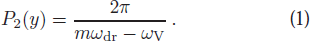
Properties of drifting subpulses can be described by the separation between two consecutive subpulses, P2, and the time required for the drift pattern to repeat, P3, with the drift-rate defined by P2/P3. Assuming emission from discrete emission areas, which are fixed to the magnetospheric plasma, implies that the value of P2 is given by the separation between two consecutive discrete areas cut by the sight-line path. Incorporating different emission states gives the following expression for the parameter as
Here, the flow rate of the plasma is

with ω dr = v dr/r and v dr is the electric drift velocity defined by E × B dip/B2, where B dip is the dipolar magnetic field proportional to 1/r3 given by Equation (A.1). The electric field represented by E has the form in different emission states given by

In Equation (3), the inductive electric field, E ind, has the form given by Equation (A.2), which is induced by the obliquely rotating magnetic dipole in vacuo, and b signifies the unit vector of the magnetic field. The flow rate due to E ind is ωind = v ind/r with v ind = E ind × B dip/B2. The electric field in relation to the corotation charge density is E pot = –gradΦcor. For y = 0, E = E cor = –( ω * × x ) × B dip is the corotation electric field giving the corotation flow rate ωdr = ωcor, where ωcor = v cor/r with v cor = E cor × B dip/B2. Here, ω* = 2π/P1 is the rotation frequency of the star, and x represents the position vector from the center of the star. The parameter ωV represents the motion of the visible point relative to the observer (see Sect. 2.2).
The traditional picture of a plasma-filled pulsar (Goldreich & Julian 1969; Ruderman & Sutherland 1975) suggests that the delay between identical repeating patterns (P3) is dependent on ωcor and ωdr. A difference between the two flow rates results in a changing pattern that repeats over several pulsar rotations. This gives
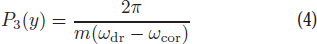
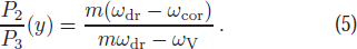
with the drift-rate given by
For an emission state, the divergence of the electric field in Equation (3) gives the charge density of the form

Here, ρGJ is the Goldreich & Julian (1969) charge density, and ρmin given by Equation (A.3) represents the minimal charge density that requires to screen the parallel electric field (to the magnetic field) in the vacuum model (Melrose & Yuen 2014). Since ρ is a function of y, the charge density in the emission region as revealed by the drifting subpulses can be deduced at different frequencies.
2.2. The Viewing Geometry
The value of y for known subpulse drift parameters can be determined accurately given a viewing geometry with known ζ, α. We adopt an approach for pulsar viewing geometry in which radio radiation is restricted to coming from the open-field region that is bounded by the last closed field-lines where emission represents the two edges of a profile window (Cordes 1978; Gil & Kijak 1993; Kijak & Gil 2003). Radiation then emits tangential to the local magnetic field-line (Hibschman & Arons 2001) of a dipolar structure and parallel to the line-of-sight direction. In this geometry, the location of the visible point at any given ψ can then be described by the spherical polar and azimuthal angles, (θV,ϕV), in the observer's frame or, (θbV,ϕbV), in the magnetic frame, with (Gangadhara 2004; Yuen & Melrose 2014)
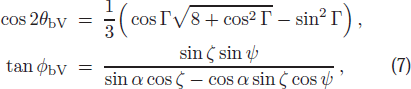
where cos Γ = cos α cos ζ + sin α sin ζ cos(ϕ – ψ), and the impact parameter is β = ζ – α. The relations of the angles θ, ϕ and θb, ϕb are given by

or

The transformation matrices between the observer and the magnetic frames are given in Appendix
Emission can be seen only when the trajectory of the visible point is inside the open-field region. This introduces the dependence of the visible point on height such that the height is minimum for emission coming from the last closed field-lines. Emission that originates from inside the open-field region would correspond to a higher height for each open field-line. The ωdr apparent to an observer is the components projected onto the trajectory of the visible point at locations defined by Equation (7) and hence it is dependent on ζ and α.
2.3. Gaps and Drifting Subpulses
In an obliquely rotating magnetosphere, the magnetic field is time-changing and
E
∥ = 0 cannot occur everywhere (Melrose & Yuen 2012). This implies the existence of a region where
E
∥ ≠ 0, known as a vacuum gap, and field-lines that pass through it are not equipotential. This gives rise to a potential difference, Φ, that changes through the gap, and the frozen-in condition does not hold. The plasma flow varies across the gap, and the Ruderman & Sutherland (1975) model assumes that the plasma flow rate is different below and above the gap with the latter at a lower angular speed than corotation. From Equation (2), this implies variation of ωdr = ωcor (y = 0) from below the gap to  above the gap, where 0 < y' ≤ 1. A feature of this gap model relates to the drifting of subpulses in an obliquely rotating magnetosphere. The systematic motion of the subpulses across the profile window implies azimuthally dependent structures drifting at an angular speed different from corotation. A possible interpretation in terms of a gap involves Φ that changes from being independent of ϕb
below the gap to ∝ cos (mϕb) above the gap (Melrose & Yuen 2016). This is due to an existence of a standing wave at a spherical harmonic of degree m producing an alternating structure of overly and sparsely dense areas of plasma around the magnetic axis (Clemens & Rosen 2004; Gogoberidze et al. 2005). Development of such azimuthal dependent structures requires an instability, and several have been suggested which involves a shear force leading to a diocotron instability in the plasma (Kazbegi et al. 1991; Pétri et al. 2002; Fung et al. 2006).
above the gap, where 0 < y' ≤ 1. A feature of this gap model relates to the drifting of subpulses in an obliquely rotating magnetosphere. The systematic motion of the subpulses across the profile window implies azimuthally dependent structures drifting at an angular speed different from corotation. A possible interpretation in terms of a gap involves Φ that changes from being independent of ϕb
below the gap to ∝ cos (mϕb) above the gap (Melrose & Yuen 2016). This is due to an existence of a standing wave at a spherical harmonic of degree m producing an alternating structure of overly and sparsely dense areas of plasma around the magnetic axis (Clemens & Rosen 2004; Gogoberidze et al. 2005). Development of such azimuthal dependent structures requires an instability, and several have been suggested which involves a shear force leading to a diocotron instability in the plasma (Kazbegi et al. 1991; Pétri et al. 2002; Fung et al. 2006).
2.4. Observable Emission Region
The interpretation of drifting subpulses in terms of emission from m discrete areas each fixed to the magnetospheric plasma implies that the emitting areas flow with the same angular velocity as the plasma. Drifting of subpulses then corresponds to the discrete areas drifting relative to corotation with the same flow rate of the plasma in an emission state. In our method, the allowed emission states are of the form defined by Equation (2). For y > 0, ωdr ≠ ωcor and the plasma flow is not in corotation and a relative speed exists between the two causing changes in longitudes of the subpulses in successive pulses, which gives rise to a systematic pattern that drifts across the profile window. Non-drifting subpulses would imply that plasma in corotation with the star with the electric drift velocity in the region can be induced by the corotation electric field (Hones & Bergeson 1965; Allen 1985; Michel & Li 1999). This suggests that corotation (y = 0) is merely another emission state in which the drift-rate is zero. From Equations (1), (4) and (5), drifting subpulses with specific values of P2, P3 and drift-rate correspond to an emission state of particular y value. The associated emission properties for the emission state are defined in relation to the values of m and ρ at the location in the emission region where the subpulse emission is detected at the observing frequency.
3. The Simulation and results
Both the subpulse drift parameters (P2 and P3) and the pulsar viewing geometry are required for the simulation. For the latter, only a few pulsars have been determined with both ζ and α of high accuracy. We search for pulsars that exhibit drifting subpulses at two frequencies centered at 326 MHz and 1429 MHz, with single drift-band at each frequency, in the papers by Weltevrede et al. (2006, 2007). They are then cross-referenced with the papers by Lyne & Manchester (1988), Everett & Weisberg (2001) and Mitra et al. (2016) for ζ and α. We obtain seven such pulsars and their details are shown in Table 1. For easy references, the value of P3 and the drift-rates for each pulsar are given in columns (2) and (3), respectively, in Table 2. Note that PSR B1933+16 exhibits drifting subpulses of an opposite sign at different frequencies. We assume the conventional notation that positive drift-rate signifies subpulses arriving later in consecutive pulses and vice versa for the negative drift-rate. The coverage of α in our sample is from 17° to 125°, and the rotation period, P1, is between 0.27 and 1.87 seconds.
Table 1. List of the Seven Pulsars and Their Parameters for the Viewing Geometry Used in This Paper
| PSR | P1 (s) | ζ° | α° | Δψ° (326 MHz) | Δψ° (1429 MHz) |
|---|---|---|---|---|---|
| B0136+57 | 0.2725 | 62.4 | 53.7 | 10 | 10 |
| B0823+26† | 0.5307 | 95.87 | 98.9 | 20 | 10 |
| B1717–29 | 0.6204 | 33.5 | 28.9 | 30 | 15 |
| B1819–22 | 1.8743 | 21.2 | 17 | 30 | 15 |
| B1917+00 | 1.2723 | 79.4 | 78.2 | 10 | 10 |
| B1933+16‡ | 0.3587 | 123.8 | 125 | 15 | 10 |
| B2154+40 | 1.5253 | 25.1 | 22.4 | 35 | 30 |
Notes: The values of ζ and α for the pulsars are taken from Lyne & Manchester (1988), Everett & Weisberg (2001) (†) and Mitra et al. (2016) (‡), and the profile width, Δψ°, at W10 (corresponding to about 10% of the maximum intensity) from the two observing frequencies and P1 are obtained from Weltevrede et al. (2006) and Weltevrede et al. (2007).
Table 2. The Observed Subpulse Drift Parameters and the Results of Simulations
| Observation | Simulation | ||||||
|---|---|---|---|---|---|---|---|
| PSR | P3(P1) | P2/P3 (°/s) | P3(P1) | P2/P3 (°/s) | m | y | ρ(ρGJ) |
| (1) | (2) | (3) | (4) | (5) | (6) | (7) | (8) |
| B0136+57 | 6.1 ± 0.5 |

| 5.9 ± 0.2 | –25.4 ± 16.2 | 20 ± 6 | 0.083 ± 0.001 | 0.909 ± 0.001 |
| 6.5 ± 0.2 |

| 6.5 ± 0.1 | –56.5 ± 30.6 | 20 ± 6 | 0.037 ± 0.001 | 0.959 ± 0.001 | |
| B0823+26 | 5.3 ± 0.1 |

| 5.3 ± 0.1 | 11.6 ± 6.3 | 33 ± 4 | 0.086 ± 0.008 | 1.033 ± 0.001 |
| 7 ± 2 |

| 8.5 ± 0.3 | 7.6 ± 3.7 | 18 ± 1 | 0.065 ± 0.012 | 1.001 ± 0.001 | |
| B1717–29 | 2.461 ± 0.001 |

| 2.5 ± 0.1 | –7.8 ± 5.8 | 32 ± 1 | 0.058 ± 0.009 | 0.941 ± 0.009 |
| 2.45 ± 0.02 |

| 2.45 ± 0.01 | –7.6 ± 1.7 | 17 ± 1 | 0.012 ± 0.001 | 0.988 ± 0.001 | |
| B1819–22 | 16.9 ± 0.6 |

| 16.9 ± 0.4 | –0.7 ± 0.4 | 23 ± 2 | 0.037 ± 0.003 | 0.963 ± 0.003 |
| 9.8 ± 0.6 |

| 9.8 ± 0.3 | -0.57 ± 0.14 | 21 ± 1 | 0.002 ± 0.001 | 0.998 ± 0.001 | |
| B1917+00 | 7 ± 2 |

| 6.2 ± 1.1 | 6.1 ± 3.1 | 27 ± 2 | 0.098 ± 0.001 | 1.226 ± 0.002 |
| 7.8 ± 2 |

| 7.2 ± 1.1 | 4.7 ± 2.6 | 21 ± 2 | 0.064 ± 0.001 | 1.148 ± 0.001 | |
| B1933+16 | 6.6 ± 0.9 |

| 6.4 ± 0.6 | -46.3 ± 23.7 | 21 ± 3 | 0.077 ± 0.004 | 0.923 ± 0.001 |
| 2.4 ± 0.3 |

| 2.4 ± 0.2 | 291.8 ± 130.8 | 24 ± 2 | 0.062 ± 0.002 | 0.993 ± 0.001 | |
| B2154+40 | 5 ± 1 |

| 4.9 ± 0.5 | 16.5 ± 7.7 | 25 ± 2 | 0.048 ± 0.001 | 0.956 ± 0.001 |
| 3.1 ± 0.8 |

| 2.9 ± 0.5 | 40.3 ± 20.9 | 22 ± 2 | 0.077 ± 0.001 | 0.929 ± 0.001 | |
Notes: Subpulse drift parameters obtained from observations are given in columns (2)–(3), and the corresponding simulated values are listed in columns (4)–(5). Note that the drift-rate is expressed in degrees per second. The upper and lower rows for each pulsar represent observing frequencies at 326 MHz and 1429 MHz, respectively. The corresponding weighted values of m and y are given in columns (6)–(7), and the charge density at each frequency is given in units of the Goldreich-Julian value in the last column.
The P2, P3, and the drift-rate are simulated for each of the two observing frequencies within the respective profile width (Δψ°) without assuming any connections between the two frequencies other than using the same ζ, α of the pulsar. Equations (1), (2), (4) and (5) are used to search for the values of y and m that give matching values for each combination of P2, P3 values and the associated drift-rates within the reported uncertainties. Specifically, for all values of m between 5 and 45, in step of 1, and y between 0 and 1, in step of 10−4, the values of ωcor and ωind in Equation (2) (hence P2 and P3) are determined for each pulse phase separated by 0.1° across the profile width at the locations defined by the trajectory of the visible point assuming β is minimum at ψ = 0°. The m and y values that give matching values of P2, P3 and drift-rate are recorded. A weighted average is then performed on all identified m and y values based on the corresponding P3 as it has the least uncertainty. Any simulated P3 value that falls within the uncertainty of the measured P3 value will receive a weight proportional to 1 – g, with g represents the interval between the measured and simulated values, normalized by the uncertainty. Once the y value is determined for drifting subpulses at a frequency, the ρmin/ρGJ is calculated for each pulse phase separated by 0.1° across the profile width along the trajectory of the visible point, then averaged to give the result. We find that the values of y and m change as the viewing geometry (ζ, α) changes, but they are weakly dependent on the profile width. The results of simulations for P3 and the drift rate for the drifting subpulses in each of the pulsars are shown in columns (4) and (5) in Table 2. The simulated values are consistent with the observations within the uncertainties.
Our results show that drifting subpulses in a pulsar observed at different frequencies demonstrate preference for different y values. In addition, none of the y value is zero indicating that the plasma is not in corotation in the emission region. The greatest deviation from corotation is found in PSR B1917+00 at 326 MHz whereas the least deviation occurs in PSR B1819–22 at 1429 MHz. This implies that the different emission states (y ≠ 0) at different observing frequencies each possess unique ωdr that is different from ωcor resulting in the diversity of the drifting subpulses, as indicated by Equations (1), (2), (4) and (5). The average y value is 0.070 ± 0.015 at 326 MHz and 0.046 ± 0.025 at the 1429 MHz, and the overall average is 0.058 ± 0.033. In general, the subpulse number is not a constant but varies with pulsars, in consistent with some previous studies (Gil et al. 2003; Smits et al. 2007). For PSRs B1819–22 and B2154+40, which have the least two α, the values of m as revealed by the drifting subpulses at the two frequencies show preference for being similar within the uncertainties. As α increases, the emission shows preference for coming from different locations each with different numbers of subpulses, with the value of m being generally greater at lower frequency. The exception is PSR B1933+16, while similar m is predicted for PSR B0136+57. The minimum value is m = 17 ± 1 in PSR B1717–29 at 1429 MHz, and the maximum value is m = 33 ± 4 found in PSR B0823+26 at 326 MHz. The average value is 26 ± 10 at 326 MHz, whereas it is slightly lower at 1429 MHz with 21 ± 8. The overall average is 24 ± 12, which is consistent with 20 predicted by Mitra & Rankin (2008).
The charge density for the pulsars at each of the two observing frequencies is shown in the last column in Table 2. For all pulsars, ρ ≠ 1 indicates that they all deviate from the Goldreich & Julian (1969) value in consistent with y ≠ 0. In addition, the charge density does not show strong correlation with the frequency. For PSRs B0823+26, B1917+00 and B2154+40, the charge density is lower at high frequency but the opposite is predicted for PSRs B0136+57, B1717–29, B1819–22 and B1933+16. The charge density in the part of the emission region, where emission is detected, can be greater than ρGJ as in PSRs B0823+26 and B1917+00. The average charge densities are 0.993 ± 0.027 and 1.002 ± 0.022 for 326 MHz and 1429 MHz, respectively, which are similar within the uncertainties.
From our results, different emission states (different y values) correspond to unique emission properties in either the charge density or the subpulse number or both as revealed by the drifting subpulses. Furthermore, the emission states are different at different observing frequencies for a pulsar suggesting that the emission properties are frequency dependent.
4. Emission region and the parameter y
From Table 2, subpulses drift because the flow rate of the emitting plasma deviates from corotation in the emission region with a particular emission state. From the consideration of the vacuum gap (Ruderman & Sutherland 1975; Melrose & Yuen 2016), the value of y is related to height in the way that y varies from corotation (y = 0) at near the stellar surface to increasingly deviates from corotation (y > 0) as the height increases. Therefore, the value of y as revealed by the drifting subpulses represents the emission state at a particular height from which the emission from the subpulses is observed. In this section, we will investigate several properties of the emission region related to the value of y.
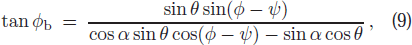
Figure 1 shows the variations in the y values as a function of α for the drifting subpulses at the two frequencies in our sample. The changes in the y values are different at different frequencies. At low frequency (blue), the y value exhibits a clear increasing trend up to α ∼ 80° implying that emission is from increasingly higher height as α increases regardless of the drift-rate and drift direction. Such trend is not clear at the high frequency (yellow) where large fluctuation is observed when α is small. As α continue to increase, both curves appear to start flattening within the uncertainties. However, unique features reveal when comparisons are made for the variations in the y values between the two frequencies. For α ≥ 28.9°, the changes in the y values demonstrate clear distinction between the two observing frequencies in such a way that greater y value is consistently associated with the low frequency. In addition, variations in the y values with α at both frequencies display similar trends regardless of the drift-rate or the drift direction. This is seen in PSRs B0136+57 and B1717–29, where the drift-rate is higher at high frequency in the former and reverse in the latter, and PSR B1933+16 with which the drift direction is different at different frequencies. This suggests that emission is from a higher height for low frequency, and vice versa for high frequency, in consistent with the frequency-to-radius mapping. However, this distinction changes as α decreases below 28.9° where the y values do not show strong correlation with the observing frequencies. For example, PSR B2154+40 displays greater y values at high frequency than that at low frequency.

Fig. 1 Plot showing variations in the y values as a function of α for the drifting subpulses observed at 326 MHz (blue) and 1429 MHz (yellow).
Download figure:
Standard imageFor subpulse drifting pulsars, the plasma revolves once around the magnetosphere relative to corotation in the time given by tc = m P3 in an emission state defined by Equation (4). Figure 2 shows a plot for the variations of tc values at the two observing frequencies as a function of P1. For our sample, the time that it takes the plasma to complete one revolution shows an increasing trend as P1 increases at low frequency. This is different for high frequency where tc fluctuates within the uncertainties. However, two distinctive trends are identified when considering the variations of tc at the two frequencies together. For P1 > 0.6 s, changes in tc at the two frequencies both demonstrate an increasing trend as P1 increases, with the value of tc being consistently higher at low frequency. However, such correlations are not clear for P1 < 0.6 s, with PSRs B0136+57 and B0823+26 both showing preferences for similar tc value at both frequencies within the uncertainties. This implies that the plasma flow in the magnetosphere of a pulsar with P1 > 0.6 s may tend to be more systematic in the sense that the plasma at low frequency takes longer time to complete one revolution. In dipolar field structure, the size of a carousel increases with height due to increased field-line spreading and hence a longer circulation time at low frequency. This is consistent with the frequency-to-radius mapping. Figure 3 shows a plot for variations in the value of y as a function of P1 at the two observing frequencies. As opposed to Figures 1 and 2, the variations in y as a function of P1 does not show clear distinction between the two frequencies. At the low frequency, a tendency of a decreasing trend as P1 increases is depicted. Comparing Figures 2 and 3 reveals that the variation in tc shows an increasing trend with decreasing y value as P1 increases. Since the value of y is related to emission height, a lower y value implies that the observable emission from the drifting subpulses is from a lower height for pulsars with large P1. However, the similar trend is not obvious for high frequency due to much larger fluctuation in the y value as shown in Figure 3.

Fig. 2 Plot showing variations of the plasma circulation times around the magnetosphere relative to corotation at the two observing frequencies as a function of pulsar rotation period. Similar to Fig. 1, 326 MHz is indicated by blue and values at 1429 MHz are shown in yellow.
Download figure:
Standard image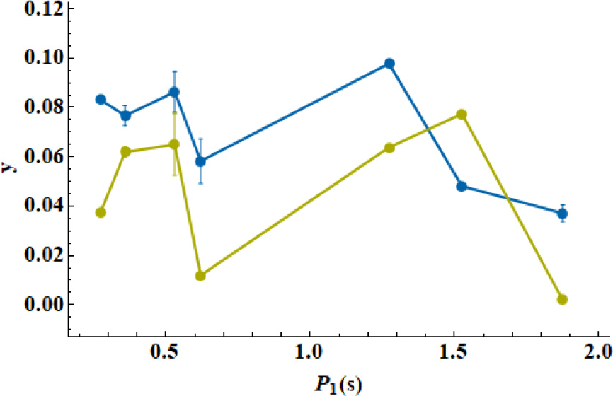
Fig. 3 Plot showing variations in the y values at the two observing frequencies as a function of pulsar rotation period. The same color code is used as in Fig. 1.
Download figure:
Standard image5. Discussion and Conclusions
We have examined the emission properties as revealed by pulsars with drifting subpulses measured at two different observing frequencies. Our investigation is based on a method that incorporates the rotating carousel model in pulsar magnetospheres of multiple emission states. In this method, radio emission is assumed coming from m discrete emission areas that are fixed to the magnetospheric plasma. The flow rate of the plasma, ωdr, is determined by the E × B drift, with E being different in different emission states, designated by the parameter y, and a change in the value of y corresponds to a change in ωdr. An emission state is defined through the parameter y in Equation (2). Subpulses drift because the plasma flow is not in corotation in an emission state, which corresponds to ωdr ≠ ωcor for y > 0. This results in a small change in the longitudinal phase in consecutive pulses which gives rise to a systematic changing pattern of subpulses across the profile window. The value of y is specified by P2, P3 and the associated drift rate based on Equations (1), (4) and (5). An emission state of a particular y value is also associated with a charge density that is defined by Equation (6). From the consideration of vacuum gaps, the value of y is correlated with height where emission from the drifting subpulses is detected. We apply the model to seven pulsars with drifting subpulses measured at two frequencies centered at 326 MHz and 1429 MHz. The model allows the identification of y and m through simulations for the P2, P3 and the drift-rate of the drifting subpulses at the two observing frequencies. The results show that y ≠ 0 in our sample indicating that the emitting plasma is not in corotation for subpulse drifting pulsars. Furthermore, the value of y is different for drifting subpulses at different frequencies in a pulsar. The corresponding charge density deviates from the Goldreich-Julian value for all pulsars and it does not show strong correlation with frequency. In general, different emission states are associated with different emission properties in the form of different subpulse number and/or charge density. We find that the changes in emission height follow frequency-to-radius mapping for pulsars with α ≳ 30°. For these pulsars, the emission height, as revealed by the value of y, increases as α increases up to about 80°, then begins to flatten as α continues to increase up to the maximum value in our sample. In addition, the value of y exhibits a decreasing trend as P1 increases at low frequency indicating that radio emission is from a lower height relative to the light-cylinder radius in long period pulsars. We find that the plasma flow is correlated with the observing frequencies only for P1 > 0.6 s in the way that the time for one complete circulation around the magnetosphere decreases as P1 decreases.
Conventional models predict the existence of a potential difference in the vacuum gap where E ≠ 0 to accelerate charge particles along the open field-lines to ultra-relativistic energy for pair production cascade, which is essential for pulsar radio emission generation (Goldreich & Julian 1969; Ruderman & Sutherland 1975; Arons & Scharlemann 1979). In general, this accelerating potential is related to the rotation period of a pulsar in the way that the former reduces as the latter increases. In this model, pulsar evolution is from short to long rotation periods and radio pulsar death is in the long period regime signified by the suppression of the pair production (Arons 2000; Zhang et al. 2000; Harding & Muslimov 2002). Since the conventional radio emission generation is suggested also underlying the mechanism for drifting subpulses (Ruderman & Sutherland 1975), the evolution and pulsar death also apply to subpulse drifting pulsars. From consideration of low frequency in Figure 3, an evolution of P1 from small to large corresponds to decreasing in the value of y, and from Figure 1, a continuing decrease in the y value corresponds to a decrease in α. This implies that the increasing in P1 as a pulsar ages corresponds to the evolution of α from large to small. Furthermore, since a lower y value indicates emission from a lower height, emission from younger pulsars will tend to come from higher heights as compared to older pulsars. In addition, emission from subpulses that show similar drifting properties is also generated at higher height in younger pulsars as with PSRs B1917+00 and B2154+40. At low frequency, the two pulsars have similar P3 and drift-rate but the corresponding y values are different with the former pulsar being greater than the latter. Assuming a similar condition at the stellar surface would suggest that the accelerating gap is 'thicker' in pulsars with large α. This implies that the emission region shrinks as a pulsar ages and the emission originates from increasingly lower height. In conventional models, two parameters are important for the pair production. One involves the distance for the electrons to travel for triggering γ-ray photons (Zhang et al. 2000), or the mean free path of the electron, le. Another parameter relates to the incident angle, θc, between the γ-ray photons and the local magnetic field, which should result in photon energy that exceeds certain threshold value (Weise & Melrose 2002). In order to maintain the pair production in older pulsars, le must reduce. However, the field-line curvature also reduces as the height decreases resulting in the diminishing of θc. Therefore, higher electron energy is required in order to maintain radio emission. However, greater electron energy implies large potential difference which is proportional to the rotation period of the pulsar. Unless different processes are involved, such as pulsars as quark stars (Xu et al. 1999; Xu 2008), our results suggest that pair production and radio emission remain in favor of young pulsars.
The distribution of each subpulse on the carousels as functions of height and α is unknown. While previous investigations show that subpulses are well-organized across the profiles, some studies also suggest different models for subpulse distribution in the emission regions which are pulsar dependent (Lyne & Manchester 1988; Rankin 1993a; Kramer et al. 1994; Manchester 1995; Esamdin et al. 2005; Smits et al. 2005; Wang et al. 2014; Dyks 2017). The diverse results obtained from some examinations of the relationship between profile width and frequency (Kijak & Gil 1998; Mitra & Rankin 2002; Chen & Wang 2014), which can be positive, negative and no correlations, suggested that profile evolution may be different for different pulsars. This also leads to the proposal that the observed changes in profile width is a byproduct of inhomogeneous emission spectra across an emission region (Chen & Wang 2014), in favor of subpulse distribution being pulsar dependent. In our model, radio emission comes from m discrete areas that are distributed around the magnetic axis. This implies that detectable emission corresponds to only the discrete areas being cut by the trajectory of the visible point forming the on-pulse region. Therefore, the profile width is dependent on the distribution of the discrete areas, and the profile edges are determined by the two locations where the trajectory enters and exits the first and last discrete areas, respectively. Furthermore, the correlation between α and the value of y suggests that the emission properties, including the distribution of the discrete areas, is dependent on the pulsar. Thus, the visible emission height relies on both the viewing geometry as well as the distribution of the discrete emission areas of the pulsar. This is consistent with the finding that the value of β is not always important for estimating the width of the core emission (Maciesiak & Gil 2011). In pure geometrical model, the determination of height is based on comparing the profile widths in dipolar field structure with the assumption that emission originates from the last closed field-lines. A prediction of the model is that observable emission is from a lower height for small β, and vice versa, which would imply the discrete areas being located near the last closed field-lines. This may be the case for PSRs B0136+57 and B1717–29, with which the β and the average y value of the former are greater than that of the latter implying that emission height is higher in the former. In general, emission may not originate from the last closed field-lines and it can come from within the inner open-field region. Our assumption that emission comes only from the open-field region introduces a dependence of height on the distribution of the discrete areas in the way that emission appears to come from higher heights if the trajectory cuts the discrete areas that are distributed in the inner open-field region. This may be the case for PSR B1917+00 where β is small suggesting emission is from close to the magnetic axis. For distribution of discrete areas on carousels with different dimensions at different frequencies, some of the discrete areas may move out of the trajectory resulting in similar profile width at different frequencies, but different y values, as may be the case for PSRs B0136+57 and B1917+00. In its present form, our model is incapable of predicting the distribution of the discrete emission areas for a pulsar. Such investigation of the topology of carousels in three dimensions would require plasma information in the emission process and polarization details at multiple frequencies which we plan to explore in a future paper.
Establishing a broadband nature of phenomenon is important for understanding the evolution of the emission region with frequency. It also makes possible for an appropriate choice of pulsars for more in-depth and sensitive observations. This can be achieved in a larger sample of pulsars with more accurate determination of the ζ and α and with drifting subpulses measured at multiple different frequencies. In addition, Figures 1 and 3 demonstrate that the emission state in an emission region is not constant but is closely related to α. This implies that drifting subpulses can occur in pulsars with different α meaning that the phenomenon is common. This is consistent with the recent detection of the phenomenon in Vela pulsar (Wen et al. 2020). However, it may be that the drift-rate of subpulses is too low making the detection difficult in some pulsars. The encouraging results from Weltevrede et al. (2006, 2007) suggest that a large number of pulsars with drifting subpulses is awaiting to be discovered. With super-large radio telescopes such as the 500-m Aperture Spherical radio Telescope (FAST) and the future Square Kilometer Array (SKA), it is hopeful (Wang et al. 2019) that larger sample size will be available for study and hence deepening our knowledge of pulsar radio emission mechanism and the associated emission geometry.
Acknowledgements
We thank the XAO pulsar group for useful discussions. The authors would like to thank the referee for valuable comments which have improved the presentation of the manuscript. RY is supported by the National Natural Science Foundation of China (grant Nos. U1838109, 11873080 and 12041301), the open program of the Key Laboratory of Xinjiang Uygur Autonomous Region under grant No. 2020D04049, the 2018 Project of Xinjiang Uygur Autonomous Region of China for Flexibly Fetching in Upscale Talents and partly supported by Xiaofeng Yang's Xinjiang Tianchi Bairen project and CAS Pioneer Hundred Talents Program.
Appendix A:: The electromagnetic fields
For an obliquely rotating magnetic dipole in vacuo, the dipolar magnetic field is defined by
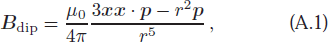
and the corresponding inductive electric field is given by
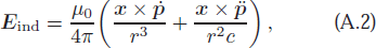
where μ0 and c are the vacuum permeability and the speed of light, and
x
and r represent the position vector and radial distance measured from the center of the star, respectively. Here,
p
is the dipole moment. The vectors on the right-hand side in both Equations (A.1) and (A.2) can be defined in either the magnetic or the observer's frame. For example, following the conventions in Appendix B,
p
is along  in the magnetic frame. The corresponding transformation for the vector relative to the rotation axis is then performed using Equations (B.2) and (B.4).
In the model for pulsar magnetospheres of multiple emission states, the charge density required to screen the parallel component of the inductive electric field (to the magnetic field), E ind∥, is obtained by taking the divergence of the electric field, given by

Here, b is the unit vector of the magnetic field, and ε0 is the vacuum permittivity. The Goldreich and Julian charge density is given by ρGJ = ε0div E cor, with E cor defined in Section 2.1.
Appendix B:: Coordinate transformations
In Cartesian coordinates, the magnetic and rotation axes of a pulsar may be arranged in the way that  and
and  , respectively, with unit vectors given by
  and
and  . The transformation between the unit vectors is given by
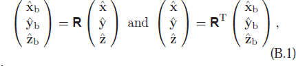
where
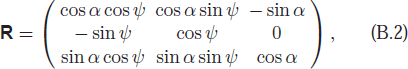
and the transpose of
R
is signified by
R
T. The corresponding unit vectors for radial, polar and azimuthal in spherical coordinates are represented by  and
and  , and
, and
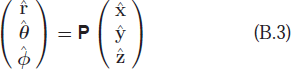
with
represents the transformation.