Abstract
In deep space exploration, it is necessary to improve the accuracy of frequency measurement to meet the requirements of precise orbit determination and various scientific studies. A phase detector is one of the key modules that restricts the tracking performance of phase-locked loop (PLL). Based on the phase relationship between adjacent signals in the time domain, a novel phase detector is presented to replace the arctangent phase detector. The new PLL, which is a closed loop signal correlation algorithm, shows good performance in tracking signals with high precision and the tracking accuracy of frequency of 1 second integration is close to Cramer-Rao lower bound (CRLB) when setting proper parameters. Actual data processing results further illustrate the excellent performance of the novel PLL.
Export citation and abstract BibTeX RIS
1. Introduction
Signal correlations have been used for Doppler shift measurements since long time ago. For example, in the application of measuring blood flow velocity, the phase increment of the latter signal relative to the previous signal can be calculated through the autocorrelation of signals at adjacent moments, and the blood flow velocity can be obtained (Bonnefous & Pesqué 1986). Signal correlations are also widely used in other fluid velocity measurements (Cadel & Lowe 2015). Signal correlations also have some important applications in other fields, including high precision measurement of the speed of moving objects (Hirata & Kurosawa 2012), and microwave Doppler sensors (Khablov 2017).
The cross-correlation method is often used in astronomical research to measure the relative velocity of celestial bodies. By calculating the cross-correlation between the signal of celestial bodies and the signal of the template, the velocity of celestial bodies can be measured (Allende Prieto 2007). In the technical field of astronomy, the key principle of very long baseline interferometry (VLBI) is also the cross-correlation method. The delay difference between the signals of the same detector received by different VLBI stations can be measured through the cross correlation operation, and then the delay difference can be used for the orbit determination (Schuh & Behrend 2012).
Recently, a cross correlation has been used in carrier tracking for deep space exploration, and an open-loop cross-correlation Doppler frequency shift estimation algorithm has been obtained. The frequency measurement results of this method are compared with that of the actual Radio Science Receiver, and the tracking accuracy of Doppler frequency is slightly improved (He et al. 2020). However, the shortcoming of the open-loop crosscorrelation method is that when the sampling rate of the signal is high, the calculation amount of the algorithm is too large, and the measurement accuracy of the algorithm will be significantly reduced at high dynamics.
Phase-locked loop (PLL) is a classical high precision carrier tracking method, which is widely used in radar, deep space exploration and other fields. In PRIDE (Duev et al. 2016) (Planetary Radio Interferometry and Doppler Experiment) of Joint Institute for VLBI in Europe (JIVE), phase-locked loop is used in carrier tracking. Shanghai Astronomical Observatory also developed a Doppler measurement method by a second order phaselocked loop (Ma et al. 2016). In order to realize high precision Doppler frequency and phase estimation, and to meet the needs of further distance and richer forms of deep space exploration, it is necessary to improve tracking performance of PLL.
In our study, a phase detector is taken as the key module to improve the performance of PLL. At present, an arctangent phase detector is most widely used in PLL due to its largest convergence range and the smallest phase error (Di et al. 2014). As is seen in Figure 1, the function of the traditional phase detector is to extract the phase difference between the input signal X1(t) and the reconstructed signal X2(t). Because the coherence of adjacent signals' spectrums can be used to identify phases, therefore, a novel phase detector can be designed to replace the arctangent phase detector in PLL. We refer to the newly designed detector as "coherent phase detector". Compared with the open-loop cross-correlation algorithm, the new closed-loop signal correlation algorithm proposed in this paper can greatly reduce the computation especially when sampling rate is high.
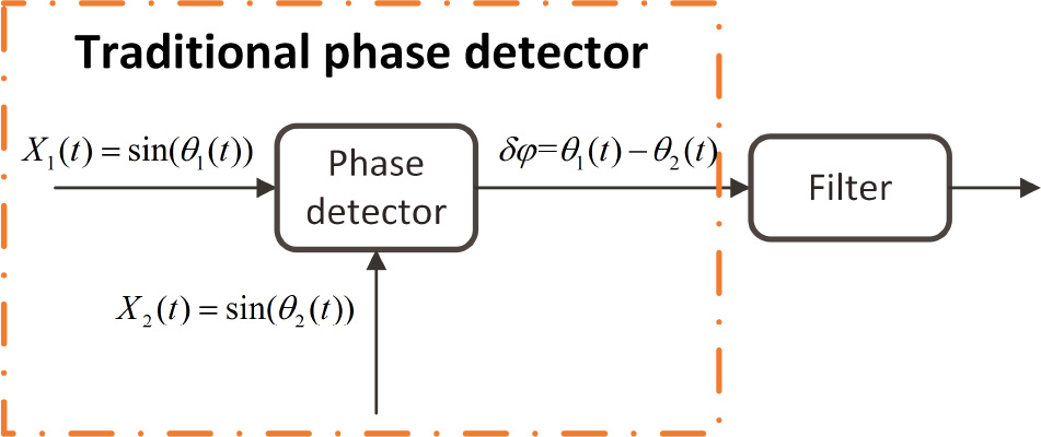
Fig. 1 The phase discrimination diagram of the traditional phase detector.
Download figure:
Standard imageThe first section of this paper is introduction. Second, the realization of the coherent phase detector is detailed presented. Third, Cramer-Rao lower bound (CRLB) and optimal tracking accuracy of frequency are calculated. Fourth, simulation results are given to verify this proposed algorithm. Fifth, the processing results of Longjiang-2 are shown. Finally, we give a summary.
2. Realization of coherent phase detector
The corresponding structure of PLL based on a coherent phase detector is shown in Figure 2. The input signal and the reconstructed signal of the two branches are respectively mixed, and the mixed signal then pass through integrate/dump filter. The difference of phase difference between input signal and reconstructed signal at adjacent moment could be obtained by coherent phase detector. The noise in the output of phase detector is filtered out by a loop filter. The reconstructed phase is obtained by integrator and can be used to reconstruct signal. Frequency initialization is performed by using the open-loop frequency maximum likelihood estimation method (Satorius et al. 2003). In most cases, this method can make the estimation accuracy of the initial frequency within 1 Hz when Fourier transform (FFT) resolution is set to 1 Hz, which is conducive to frequency acquisition.
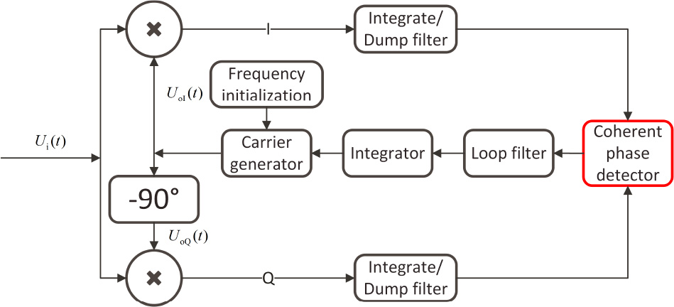
Fig. 2 Phase-locked loop structure based on coherent phase detector.
Download figure:
Standard imageFigure 3 shows the basic principle of a coherent phase detector. The time lengths of d1(t) and d2(t) are equal. In Figure 3, it assumes that the phase increment of the latter signal d2(t) relative to the preceding signal d1(t) is Δφ and Δφ can be identified. So a new type of phase detector is obtained. This kind of phase detector can also be used as a key module of phase locked loop. The derivation process of the coherent phase detector is shown in Figure 3. Let the form of the input signal be

The actual expression of the input signal is X(t) = Acos(2πfc
t + ϕ), fc is carrier frequency, ϕ is initial phase. In the expression of Equation (1), we take the initial phase ϕ as part of 2πft. Over time, the value of f will approach the real carrier frequency fc and both become nearly the same. The form of Equation (1) is convenient for subsequent derivation. The reconstructed in-phase (I) component of input signal is  , while the reconstructed quadrature (Q) component is
  . After mixing the input signal and the in-phase component, the output is
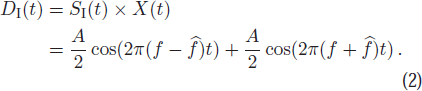
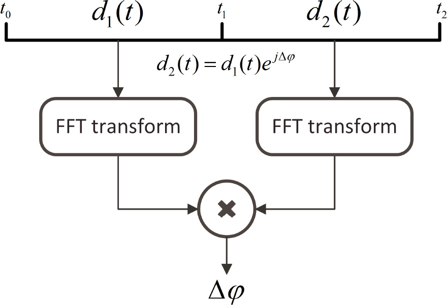
Fig. 3 Basic principle of designing coherent phase detector.
Download figure:
Standard imageAfter mixing the input signal and quadrature component, the output is
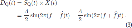
We assume the period used in integrate/dump filter in Figure 2 is T0, and the function is summing up the data for each continuous period of time (T0). Fs is the sampling rate of the data at the output of integrate/dump filter. If T0 is set to 25 μs, it means that the 25 μs data is accumulated to get an output data. The effect of integrate/dump filter is equivalent to a low-pass filter, which can eliminate interference signals of high frequency. Therefore, the signal form after integrating and dumping operation can be expressed as follows. The in-phase component
The quadrature component
Construct a variable
Discrete form of Z(t) is
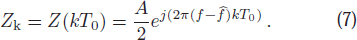
Phase compensation is then performed for Zk. Compensation formula is

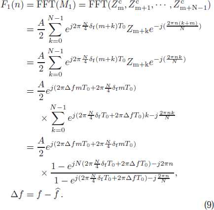
The spectral resolution of the Fourier transform of M1 is  and N is the length of M1, M1 is defined below. Phase compensation can shift the spectrum of the sequence. The reason for the phase compensation is that the position of the spectral line with the maximum amplitude can be at the non-edge of the obtained coherent spectrum, which is conducive to further signal processing.
Define  . First, wavelet soft threshold denoising is used to preprocess M1 to eliminate part of the noise and the discrete Meyer wavelet (Dmey) is selected here. Then apply Fourier transformation to M1, the detail expression is
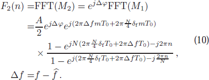
Define  , M2 is next to M1 and both have equal length. Assume that M2 = ejΔφ
M1. Wavelet soft threshold denoising is also used to preprocess M2 to eliminate part of the noise. Then Apply FFT transformation to M2, the expression is
, M2 is next to M1 and both have equal length. Assume that M2 = ejΔφ
M1. Wavelet soft threshold denoising is also used to preprocess M2 to eliminate part of the noise. Then Apply FFT transformation to M2, the expression is
Multiply F1(n) by F2(n), then a coherent function of two frequency spectrums is obtained.
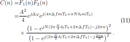
It can be obtained from the analysis of Equation (11) that, when  , the amplitude of C(n) is largest. Then we obtain that
  and
and  . In this way, a relationship can be further obtained from Equation (11).
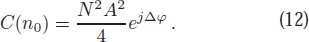
n0 is the frequency point corresponding to the maximum amplitude of C(n). In this case, the relative phase increment between M2 and M1 is argument of C(n0). In fact, we know that the frequency resolution  is large. At this time, there is still some small deviation between the obtained value n0 and the actual value n, and n satisfies the equation
  . For this reason, two points adjacent to n0 are also used to calculate Δφ. For the complex Fourier transform of N points,
  represents positive frequencies,
  represents negative frequencies. The actual negative frequency has to be subtracted by N + 1. Therefore, the Δφ calculation strategy is as follows:
If 

If  , then
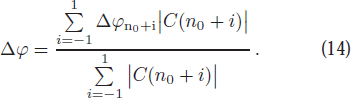
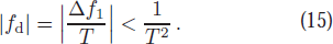
Δφ can be used as the input of the loop filter. On the other hand, in order to prevent integer cycle ambiguity to appear in phase discrimination, coherence time T, that is, the corresponding time length of M1 or M2 used in coherent computation should satisfies inequality |2πΔf1 T| < 2π and Δf1 is the relative frequency increment between M1 and M2. Therefore, it is necessary to ensure that the first derivative of the Doppler frequency fd satisfies the relation
As is seen in Figure 4, θ1(t) is the phase of the input signal, θ2(t) is the phase of the reconstructed signal. Compared to the traditional phase detectors shown in Figure 1, the phase difference δφ between input signal and output signal is not directly obtained by coherent phase detector. Instead, the difference of phase difference δφ at adjacent moments is obtained. The discrete linear structure of PLL in this paper is shown in Figure 5.
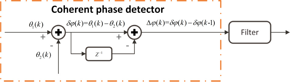
Fig. 4 Diagram of coherent phase detector.
Download figure:
Standard image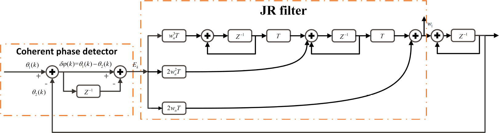
Fig. 5 Linear discrete structure of PLL.
Download figure:
Standard imageThe measured Doppler frequency is
The transfer function of phase error
When the input phase is θ(t) = 0.5at2, in which a is a constant, the steady-state error is
Although the JR (Jaffe Rechtin) filter is a second-order filter, the PLL is still a second-order PLL due to the use of coherent phase detector. The closed-loop transfer function of the phase-locked loop is
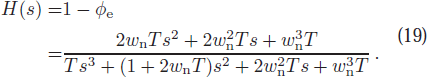
The calculation formula of loop noise bandwidth (Wang 2009) is
3. Cramer-Rao Lower Bound (CRLB) and optimal tracking accuracy of frequency
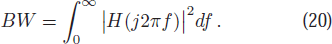
Write the input signal in another form
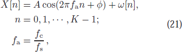
where A is amplitude, K is the number of points that are sampled independently, fs is sampling rate of original signal, fc is carrier frequency, ϕ is initial phase, and ω[n] is a Gaussian noise which mean is 0 and variance is σ2. In PLL, the accuracy of frequency estimation is almost unaffected by amplitude and initial phase. Then when calculating the CRLB of the estimation of fc, we assume that the amplitude and the initial phase are known. The derivation process of CRLB is given below.
The probability density function of X[n] is
Take the derivative of the likelihood function
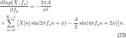
And
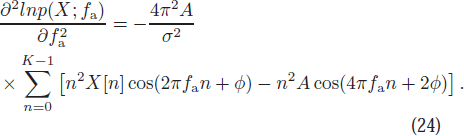
Fisher information is
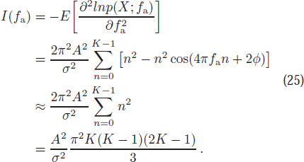
Then
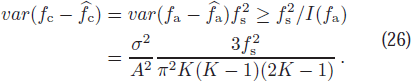
 represents an estimate of fc and
  represents an estimate of fa. Finally, the optimal root mean square (RMS) of frequency is obtained
The square root of CRLB will be used as an absolute criterion to evaluate the tracking accuracy of proposed algorithm.
4. Performance analysis
4.1. Tracking Accuracy and Robustness Analysis
Simulation parameters setting: sampling rate fs = 4 MHz, the initial frequency of the signal f0 = 1 MHz. The definition formula of the carrier to noise ratio (CNR) generated in simulation is
Here Ps is signal power, and N0 is the noise spectral density, and A is amplitude of signal, and σ2 is the variance of the noise and Ts is sampling period of input signal. For phase locked loop based on coherent phase detector, the period of integrate/dump filter T0 is set to 250 μs and coherence time T, which is loop updating time, is set to 5 ms.
The phase model is defined as
The units of f0, f1, f2 are Hz, Hz s−1, Hz s−2, respectively. ϕ is the initial phase of input signal.
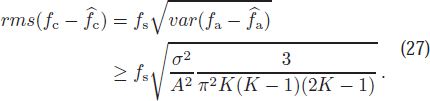
As is seen in Figure 6, the phase-locked loop algorithm based on coherent phase detector can accurately track Doppler frequency of the signal, which proves the correctness of the algorithm. Figure 6 shows the tracking accuracy of the signal frequency under different CNRs. In the simulation experiments of Figure 6, the loop noise bandwidth was set to decrease gradually from 4.35 Hz to 0.13 Hz (ωn decreases from 20 to 1) in the first 5 seconds. The data of 65 seconds were tracked each time, and when caculating tracking accuracy of frequency, that is root mean square of residual frequency, the measured frequency of the first five seconds were eliminated.
Fig. 6 RMS of residual frequency under different CNRs. Label 1 represents the results whose parameters are f0 = 1 MHz, f1 = 200 Hz s−1, f2 = 0.012 Hz s−2, ϕ = 1 rad. Label 2 represents optimal tracking accuracy of frequency which is square root of CRLB. P represents the probability of frequency being locked correctly. When analyzing P under different CNRs, 100 Monte Carlo trials were conducted for each fixed CNR and the RMS of residual frequency less than 1 Hz was believed to be correct, in which residual frequency was equal to the measured frequency minus the true frequency.
Download figure:
Standard imageIn Figure 6, when setting the loop noise bandwidth to 0.13 Hz, even though the third derivative of the phase cannot be ignored, the estimation precision of the frequency of 1 second integral still approaches the square root of CRLB. At the same time, with the bandwidth set to 0.13 Hz, the frequency of relatively high-dynamic signals can still be measured by this algorithm. The results illustrate that the measured frequency here is a nearly minimum variance unbiased estimate for the measured frequency of 1 second integration. Although the CRLB derivation assumes that the frequency is completely unknown, and in this new PLL, the frequency estimate at the previous time is a priori information of the frequency for the current second. This leads to the assumption in the CRLB derivation that the frequency is completely unknown is not entirely correct. However, in general, when set proper parameters for applications, the possible highest accuracy of the actual estimated frequency is only slightly higher than CRLB due to the long integration time of the frequency as long as 1 second. Therefore, the CRLB can still be used as an absolute benchmark to evaluate the accuracy of the measured frequency of 1 second integration. For the estimated frequency of 5 s and 60 s integration, the optimal estimation accuracy of frequency which is square root of CRLB cannot be achieved by using the current algorithm proposed by this paper.
As is seen in Figure 6, when the CNR of signal is larger than 30 dB-Hz, the signal frequency can be tracked stably under the current parameter settings. Actually, the CNR of actual data is often larger than 30 dB-Hz in deep space exploration. In addition, the dynamic of the simulation signal is large enough to basically cover the application scenarios of carrier tracking of X-band (8.4 GHz) and S-band (2.2 GHz) signals in most cases.
4.2. Computing Time
In the practical applications, the computing time of the algorithm is one of the factors concerned. The new algorithm proposed in this paper has two key parameters which affect the computation amount of the algorithm. The two key parameters are the period of integrate/dump filter T0 and loop updating time T, respectively. As T0 is set to 0.25 ms, it can meet the application requirements in most scenarios and is a typical value. Therefore, T0 is set as a constant value when analyzing the computing time, and then the computing time under different T values is compared.
Since the number of phase discriminations is inversely proportional to T, when T is smaller, the number of phase discriminations per second is larger and the amount of calculation is greater. For the method proposed here, its weak signal tracking ability and high dynamic tracking ability are often contradictory to each other. Although a large T value means less computation and stronger weak signal tracking ability, it also means a poor high dynamic tracking ability. Therefore, the selection of T is the result of trade off of all factors.
In addition, the algorithm can be written in C programming language or other programming languages to further reduce the computing time.
5. Actual data processing
In order to further verify the reliability of the new proposed Doppler measurement algorithm, the observation data of Longjiang-2 on 2018 August 24 with 2 bits sampling were processed in this paper. Longjiang-2 is a minor satellite launched alongside Queqiao relay satellite of Chang'e-4. The sampling rate and bandwidth of the signals received by the telescopes after down-conversion are 4 MHz and 2 MHz, respectively. During the tracking process, set the loop noise bandwidth to 0.13 Hz when the loop becomes stable. In observation, the VLBI station alternate observations of Longjiang-2 and radio source. These data were observed by VLBI station in Kunming.
Figure 8 shows the results of estimated CNR of the signal. The process of estimating CNR of actual signals is as follows: First, the phase of the signal is measured using the algorithm proposed in this paper. Second, the measured phase is used to compensate the raw data so that the signal energy is concentrated within 1 Hz. Third, the power spectrum of the compensated data is calculated. Fourth, the maximum value of the power spectrum is used as an estimate of the total power of the useful signal. Fifth, take some amplitude values except the maximum value in the power spectrum, and calculate its mean value as the estimate value of noise power. Finally, Equation (28) is used to calculate the estimated value of CNR of actual signal.
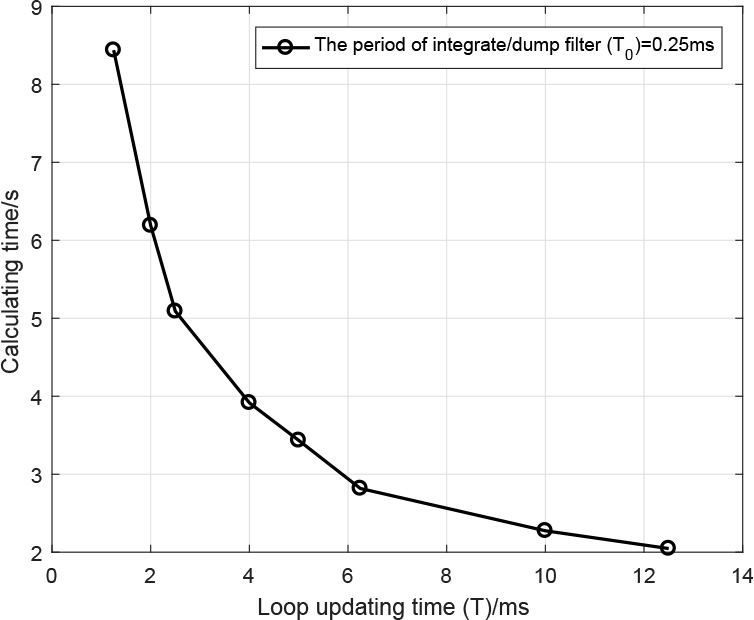
Fig. 7 Computing time is shown when processing 1 second data. The algorithm is written in MATLAB language.
Download figure:
Standard image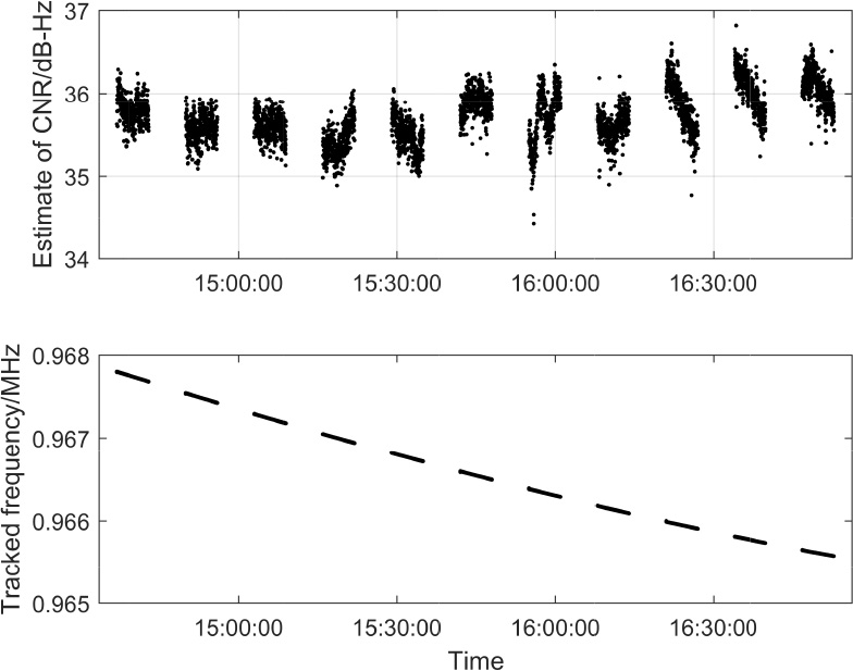
Fig. 8 The estimate of CNR and tracked frequency.
Download figure:
Standard imageThe auto power spectrums of data before and after phase compensation are both shown in Figure 9. It can be seen that the energy of signal is obviously more concentrated after phase compensation.
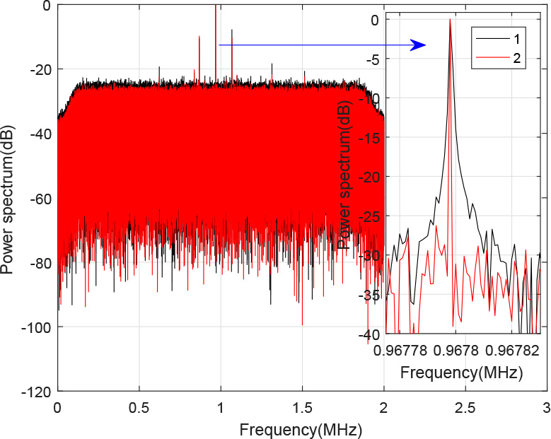
Fig. 9 The comparison of auto power spectrum of raw data and that of data after phase compensation. Label 1 represents the auto power spectrum of raw data, and label 2 represents the auto power spectrum of data after phase compensation. The auto power spectrums have been normalized.
Download figure:
Standard imageFor these observation data, Longjiang-2 operated in coherent mode while generating signal, which means that frequency standard of Longjiang-2 is hydrogen atomic clock on the ground. Because the frequency of the atomic clock is highly stable, the error introduced by atomic clock can be ignored for the measured frequency of 1 second integration. Then it can be considered that the frequency error is mainly caused by the thermal noise, and the noise caused by the ionosphere and atmosphere. Then the phase noise can be approximated as the Gaussian process. The main steps to analyze the accuracy of frequency are as follows: First, estimate the signal frequency of the 1 second integration. Second, because the loop bandwidth slowly decreases when the frequency of first 5 seconds is estimated in each scan, the estimated frequency of the first 5 seconds are removed to ensure the correctness of subsequent RMS estimation. Third, the frequency residuals are obtained by fitting the estimated frequency values with the sixth order polynomial in each scan. Fourth, the RMS of frequency residuals is calculated and this RMS can be used as estimate of accuracy of frequency.
In addition, the mean value of estimated CNRs of each scan is calculated. Then the mean value is substituted into Equation (27) to obtain the estimate of the optimal estimation accuracy of frequency which is square root of CRLB. The performance of the current algorithm is evaluated by comparing the optimal estimation accuracy with the actual estimation accuracy of frequency.
As seen in Figure 10, the RMS of frequency obtained by novel method is very close to the square root of CRLB and the relative error between them is less than 22%. This result illustrates that the estimated frequency obtained by this method is almost the minimum variance unbiased estimator when processing actual data. In addition, Shanghai Astronomical Observatory has developed an engineering software for carrier tracking (Zheng et al. 2013) and the software has been used in recent deep space exploration missions, including the first Chinese Mars exploration and Chang'e-5 lunar exploration mission. We compare the tracking accuracy of measured frequency obtained by the software with that of the new method presented in this paper. It is clear that the new method can achieve nearly 6 times higher tracking accuracy of frequency.
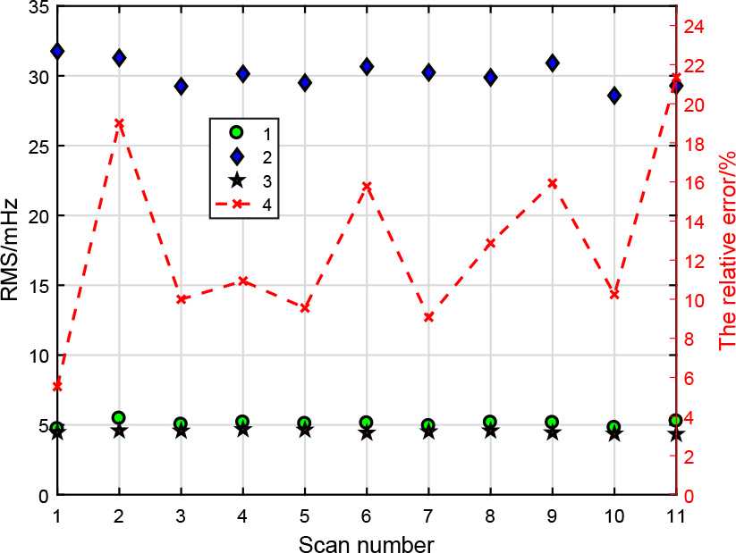
Fig. 10 The comparison of the accuracy of measured frequency obtained by different methods. Label 1 represents the accuracy of measured frequency obtained by closed signal correlation method proposed in this paper. Label 2 represents the accuracy of measured frequency obtained by Doppler measurement software which is developed by Shanghai Astronomical Observatory and has been used in carrier tracking in VLBI data processing center. Label 3 represents the theoretical optimal accuracy which is square root of CRLB. Label 4 represents the relative error between the accuracy of measured frequency obtained by new method and square root of CRLB.
Download figure:
Standard imageData from Chang'e-5 on 2020 November 28 with 2 bits sampling were recorded in VLBI data processing center. The sampling rate and bandwidth of these data are 4 MHz and 2 MHz, respectively. The differences between the velocity of precision ephemeris obtained by orbit determination and the measured velocity are shown Figure 11. The velocity residuals further illustrate that the algorithm proposed in this paper is feasible for frequency measurement. At about 14:30 Coordinated Universal Time, an orbit transfer of Chang'e-5 occurred, which resulted in the velocity residual is relatively large.
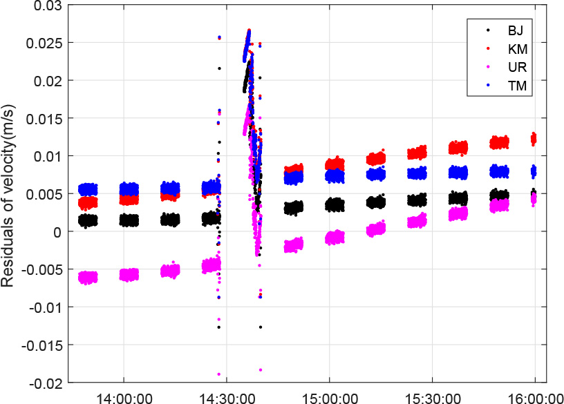
Fig. 11 The differences between the velocity of precision ephemeris obtained by orbit determination and the measured velocity. BJ represents Beijing VLBI station, KM represents Kunming VLBI station, UR represents Urumqi VLBI station, and TM represents Tianma VLBI station.
Download figure:
Standard image6. Conclusions
In this paper, a coherent phase detector is designed based on the phase relationship between adjacent signals in the time domain. Simulation and actual data processing results show that the coherent phase detector can obviously improve the estimation accuracy of Doppler frequency and the frequency estimate is close to the minimum variance unbiased estimate when setting proper parameters.
The weak signal tracking capability of the phase-locked loop can be further improved by extending the coherence time T, but dynamic tracking performance of the loop filter will deteriorate due to the increasing of time interval, and the assumption that the phase increment of the latter segment relative to the former segment become not necessarily true for the two adjacent signals. Then the dynamic tracking capability of PLL becomes poor and the frequency may not be locked. Therefore, the limitation of dynamic tracing capability should be taken into account when increasing the coherence time.
Acknowledgements
The research presented in this paper has been supported by the National Natural Science Foundation of China (11773060, 11973074, U1831137, 11703070 and 11803069), the National Key Basic Research and Development Program (2018YFA0404702), Shanghai Key Laboratory of Space Navigation and Positioning (3912DZ227330001) and the Key Laboratory for Radio Astronomy of CAS.