Abstract
As the asteroid rotational period is important to the study of the properties of asteroids (e.g., super-fast rotators have structures owing an internal cohesion (rather than being rubble piles bounded by gravity only) so as not to fly apart), constructing an effective and fast method used to search the period attracts much researchers' attention. Recently, the Bayesian generalized Lomb–Scargle (BGLS) periodogram was developed to improve the convergence efficiency of the Lomb–Scargle method. However, the result of BGLS varies with the frequency range and cannot meet the two minimum/maximum requirements for a complete rotation of the asteroid. We propose a robust BGLS-based method that efficiently determines rotational periods. The proposed method employs a polynomial series to fit folded light curves with potential periods, initially calculated using the BGLS periodogram, and adopts a merit function to estimate and refine best-fit periods. We estimate the rotational periods of 30 asteroids applying the new method to light curves from the Palomar Transient Factory. Results confirm the effectiveness of the BGLS-based method in deriving rotational periods from ground-based observations of asteroids. Further application of the BGLS-based method to sparse light curves, such as Gaia data, is discussed.
Export citation and abstract BibTeX RIS
1. Introduction
"Asteroids have been viewed as remnants of planetary formation" (Demeo & Carry 2014) and are therefore important in our understanding of the evolution of the Solar System (Izidoro et al. 2016). Combining the information on the rotational period of asteroids and their corresponding size, it can help to distinguish the interior structures of asteroids (e.g., monoliths, rubble piles, and shattered but coherent objects) (Harris 1996; Bagatin et al. 2018; Parker et al. 2008). Additionally, the spin rate distribution generated by an amount of asteroid rotational periods provides information on the size and location in the main asteroid belt (e.g., "the spin rate distributions of asteroids of 3 < D < 15 km in size show a steady decrease along frequency for f > 5 rev/day, regardless of the location in the main belt") (Chang et al. 2017).
Nowadays, more and more surveys have been conducted or are planned in the near future for asteroid discovery (e.g., CSS, PS1, ATLAS, and LSST), and such surveys provide hundreds of thousands of sparse asteroid light curves, a more efficient way of measuring rotational periods is thus essential (Law et al. 2009; Perley et al. 2020; Prusti et al. 2016). An accurate estimate of periods can help to obtain other precise parameters (such as the parameters of asteroid shape), because the rotational period is a significant part of complex inversion research like convex inversion and the use of the Cellinoid model (Kaasalainen et al. 2012; Lu et al. 2016).
Generally, besides the second-order Fourier series, one of the widely used methods adopted in quickly deriving the rotational periods of asteroids from light curves (Harris et al. 2014; VanderPlas & Ivezic 2015; Waszczak et al. 2015), another popular approach of predicting the rotational period of the asteroid is Lomb–Scargle (LS, the first-order Fourier series) (Lomb 1976; Scargle 1982). The Bayesian generalized Lomb-Scargle (BGLS) periodogram (Mortier et al. 2015) is an extension of the LS method for the analysis of periodic photometric time series and is more efficient compared with LS in obtaining periods. A major characteristic of BGLS is that it describes the probability distribution to present a full sine function with the specific frequency in the data, which cannot meet the two minimum/maximum requirements for a complete rotation of the asteroid. Besides, the result of BGLS will vary with the preset range of frequency. Therefore, the BGLS is not appropriate for direct use in searching for the periods of asteroids from light curves. The present article introduces a BGLS-based method for finding the best-fit rotational period. By applying the method to Palomar Transient Factory (PTF) observations, we present an estimate of rotational periods for 30 asteroids and obtain results that are consistent with the results of other research. Furthermore, as more sparse light curves are made on space missions, such as the Gaia mission, we apply the BGLS-based method to search for the best-fit period of (216) Kleopatra from Gaia sparse light curves. Although it is difficult to obtain the period from sparse data through spectral analysis, the proposed method derives the correct rotational period for (216) Kleopatra. This shows the potential application of the BGLS-based method to sparse light curves, such as Gaia data.
The remainder of the paper is organized as follows. First, basic knowledge of the LS method and its extensions is presented in Section 2. Subsequently, the asteroid light curve is described in Section 3 and the proposed BGLS-based method is illustrated in detail in Section 4. The folded light curves and merit function are presented in this section. Following its description in Section 5, the proposed method is applied in searching for the rotational periods of 30 asteroids from PTF observations and the case of sparse light curves for (216) Kleopatra is discussed. Finally, conclusions and directions of future work are presented in Section 6.
2. LS and BGLS Methods
Deriving the rotational period is a significant part in the inverse process from the observed photometric data of asteroids. The LS method is widely adopted to analyze frequencies of time series and to search for best-fit periods from light curves, especially in the case of unevenly sampled data (Lomb 1976; Scargle 1982).
However, the original LS method does not include the weight of data errors or consider the constant offset effect due to hardware. Studies have investigated these shortcomings (Ferraz-Mello 1981; Cumming et al. 1999; Zechmeister & Kürster 2009) and proposed the generalized LS (GLS) method (Zechmeister & Kürster 2009). Nevertheless, all methods face a drawback owing to the expression of arbitrary power. This shortcoming makes it difficult to compare peaks. To better evaluate relative probabilities among peaks, Bretthorst (2001) generalized the LS according to Bayesian probability theory (i.e., the BLS method). The BLS is much more efficient than the traditional LS in finding best-fit rotational periods.
In 2015, Mortier et al. (2015) proposed a Bayesian formalism for the generalized Lomb–Scargle periodogram (i.e., the BGLS method) by combining GLS and BLS, such that the result is intuitive and unique. When adopting the BGLS, a full sine function model that describes the periodic signal in time series data is defined as
where yi
is the data point corresponding to the time ti
, A and B are respectively cosine and sine amplitudes, f is the given frequency, θ is an arbitrary phase offset and "was chosen by Lomb to make the sine and cosine model functions orthogonal on the discretely sampled times" (Bretthorst 2001). γ is the data offset, and  i
is the noise at time ti
(Forbes et al. 1978; Press et al. 2007). This noise is per time ti
Gaussian–distributed around 0 with a standard deviation of σi
, which is the estimated uncertainty on the data at time ti
(i
∼ N(0,σi
)). Given data
i
is the noise at time ti
(Forbes et al. 1978; Press et al. 2007). This noise is per time ti
Gaussian–distributed around 0 with a standard deviation of σi
, which is the estimated uncertainty on the data at time ti
(i
∼ N(0,σi
)). Given data  (where N is the number of observations) and prior knowledge I, the best-fit frequency corresponding to the largest value of the posterior probability P(f |D, I) is obtained:
The BGLS method has advantages in implementation and is appropriate for both unevenly and evenly sampled data; e.g., ground-based light curves and space-based light curves and it also inherits the advantages of the general Bayesian method, which are "more flexible models, more principled treatment of nuisance parameters related to noise in the data, and the ability to make use of prior information in a periodic analysis" (VanderPlas 2017). Furthermore, it performs well in searching for the best-fit period using periodic photometric data, especially for sparse light curves even when the limited dataset contains few observations.
However, as mentioned above, BGLS is a full sine function model. According to a simpler shape model of the asteroid (i.e., the ellipsoid model shown as Fig. 1) (Karttunen 1989; Karttunen & Bowell 1989), the light curve of such an ellipsoid is a double-peaked sinusoid. Even for the cellinoid model (i.e., an extension of the traditional tri-axis ellipsoid shown in Fig. 2), the light curve of that should have two maxima or two minima in one rotational period. The result searched by the BGLS cannot meet the requirement for a complete rotation of the asteroid. Moreover, the BGLS will get different results due to different preset frequency ranges. Hence, the BGLS is affected largely by the intervals used in the initial search of the frequency range. It is thus time-consuming to preliminarily set an optional frequency interval when searching rotational periods of a huge number of asteroids or searching rotational periods from a sparse light curve collected for months. Therefore, we need to modify the BGLS method before we use it to estimate the asteroid rotational period.

Fig. 1 Ellipsoid shape model.
Download figure:
Standard image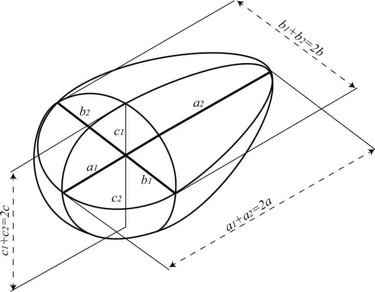
Fig. 2 Cellinoid shape model.
Download figure:
Standard image3. Asteroid Light Curves
In this article, the periodic variability term due to rotation M (corrected magnitude) is handled with different forms in PFT data and Gaia data. For PTF data, the M is modeled as

where m is the apparent magnitude, H is the absolute magnitude, r and Δ are respectively the heliocentric distance and geocentric distance, and ϕ(α) is the phase function 1 The phase function in Equation (3) is used to simulate the scattering effect corresponding to different solar phase angles, especially covering the opposition effect. Several phase models are used to simulate the scattering characteristics by combining the opposition effect at a small phase angle and the linear relationship at a large phase angle (Shevchenko 1997; Bowell et al. 1989; Muinonen et al. 2010). In this work, the magnitude data we utilize to estimate the rotational period is extracted from Waszczak et al. (2015) and is corrected for distance and phase function. According to the workflow of Waszczak et al. (2015), the single-parameter G12 form of the Muinonen et al. model (Muinonen et al. 2010) is employed and it is expressed as

where G1 and G2 are defined as

Whereas the handling process of M for Gaia data is rewritten as
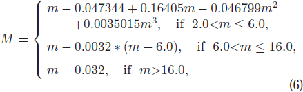
which follows the process of Evans et al. (2018).
To measure the rotation period through analyzing light curves with the BGLS method, the function of M with respect to observation time t is written as
where the definitions of parameters are the same as Equation (1), note that the phase offset parameter θ has no relationship with the phase function ϕ(α) in Equation (4), and it "was chosen by Lomb to make the sine and cosine model functions orthogonal on the discretely sampled times" (Bretthorst 2001).
4. BGLS-based Method
To mitigate the problems existing in the BGLS, in this article, we propose a BGLS-based method that is more suitable for estimating the rotational periods of asteroids. The overall process of the BGLS-based method is illustrated in detail as follows.
4.1. Process of the BGLS-based Method
A complete light curve of an asteroid covering a full rotation have two minima and two maxima. The general BGLS method only finds the period for the periodic photometric time series, which is half the asteroidal synodic period (where this period can be searched for only when the interval is set suitably). Therefore, firstly, we adopt the BGLS to search for possible periods P = [p1, p2,..., pNp ], where Np is the number of intervals that we preset. Secondly, as pre-setting the frequency range is necessary for BGLS, we think it is may be effective to evaluate multiple candidate periods obtained by different ranges (e.g., dividing a full range into multiple small ranges) to find the best-fit one. In this work, we preset 10 frequency ranges and each range contains one hour, in other words, we divide 10 hours evenly into 10 intervals 2 to search for 10 possible results adopting the BGLS. For each result, we apply a polynomial series to fit the folded light curves:
where  is the synthetic data point at time ti
while xj
is the coefficient of the polynomial. K
3
is the degree of the polynomial under the assumption that Pm
is the m-th possible rotational period.
is the synthetic data point at time ti
while xj
is the coefficient of the polynomial. K
3
is the degree of the polynomial under the assumption that Pm
is the m-th possible rotational period.
Subsequently, a new merit function
is defined for estimating the derived possible periods using the BGLS and refining the best-fit result, where m is the index of the possible periods, namely m = 1,2,...,10, and N is the number of observation points with the corrected magnitude Mi (cf. Eq. (3) and Eq. (6)).
Finally, the possible period derived using the BGLS with the smallest χ2 is the best-fit result. Furthermore, its double is the rotational period of the asteroid.
4.2. Algorithm
To sum up, we search the period step by step in each range and find one candidate period in each range (i.e., in each range, BGLS gives only one result with a corresponding probability of 1). After that, we use the polynomial fitting to find which candidate period is the best-fit. The overall process of the proposed BGLS-based method is described in Algorithm 1.
Algorithm 1. BGLS-based method
| Input: |
| Time Series, t; |
| Corrected Magnitude, M; |
| Uncertainty in apparent magnitude, err. |
| Output: |
| Best-fit rotational period, P. |
| 1: Preset 10 intervals from 0 to 10 hours. |
| 2: Search possible periods Pm (m ∈ [1,10]) adopting the BGLS periodogram in each interval. |
| 3: Fit a polynomial using Eq. (8). |
4: Calculate  using Eq. (8). using Eq. (8). |
| 5: Find the index of the minimum of χ2 and update P = Pindex*2. |
| 6: return P. |
5. Results and Discussion
5.1. Synthetic Light Curves
In this part we provide two synthetic examples that expose the effectiveness of the BGLS-based method. Supposing the longitude and latitude of the pole orientation is (0°,90°) in the ecliptic frame and the rotational period is P = 5 hr, six semi-axes are [1, 0.8, 0.9, 0.8, 0.7, 0.6], the synthetic light curves are generated in Figure 3 and Figure 5 based on the cellinoid shape with the Gaussian noise N(0, 1). The two light curves contain different observation points: 100 and 30, respectively.

Fig. 3 Synthetic Light Curves with Gaussian Noise.
Download figure:
Standard image
Fig. 4 Folded Light Curves with Gaussian Noise.
Download figure:
Standard image
Fig. 5 Synthetic Light Curves with Gaussian Noise.
Download figure:
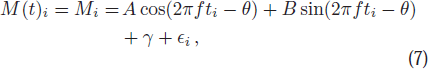
Standard imageThe results searched by the BGLS-based method are shown in Figure 4 and Figure 6. From the folded light curves figure we can learn the light curve with 100 observations shows the result 5.0336 hr whereas the sparse light curve shows the result 5.0209 hr. The error influenced by Gaussian noise is ∼ 1 min – ∼2 min. The difference of searched results is caused by the noise, obviously, we can see the noise points in the sparse light curve are smaller than those in the light curve with 100 observations.

Fig. 6 Folded Light Curves with Gaussian Noise.
Download figure:
Standard image5.2. Real Light Curves
To evaluate the performance of the BGLS-based method, we employ ground-based light curves (e.g., the PTF 4 ) and sparse space-based light curves (e.g., the second Gaia data release, Gaia DR2) to complete experiments, respectively.
The PTF is a synoptic survey conducted using a wide-field survey camera designed to search out the transient and variable sky (Law et al. 2009; Rau et al. 2009). Waszczak et al. (2015) searched all PTF (R and g-band) data from 2009-March-01 through 2014-July-18 for all numbered asteroids as of 2014-July-12 and gave the processed data in an online document (i.e., table 4 in Waszczak et al. 2015). In our work, we extracted the magnitude corrected for distance and phase function from Waszczak et al. (2015) into the period analysis.
Gaia 5 is a space observatory that measures the positions, distances, and motions of stars with unprecedented precision (Prusti et al. 2016; Perryman et al. 2001). A synthetic presentation about the case of GDR2 photometric data is given by Gaia Collaboration et al. (2018). We correct that the magnitude (G-band) also follows the work of Evans et al. (2018) (Eq. (6)).
5.3. Applications
In total, we search for the best-fit rotational periods of 30 asteroids using our proposed BGLS-based method from the light curves observed in the survey of the PTF.
An appropriate step length of the frequency should balance the computational cost and accuracy. If the step length is larger the prediction result might be not so accurate, if the step length is finer the computational cost is too huge and the accuracy of the prediction result may improve little. To find the proper step length, a numerical experiment is conducted with different step lengths of the frequency, namely 0.0001, 0.001, and 0.0025. The results are listed in Table 1. The computing time is the total time required to search for the rotational periods of the 30 asteroids. The table shows that the finest step length of 0.0001 obtains the correct periods, while the results are not satisfactory when the step length is 0.0025 although the computational cost is low. To balance the accuracy and computational cost, we suggest a step length of 0.001 in the large-scale searching of rotational periods of a huge number of asteroids.
Table 1. The Rotation Periods Obtained Using Different Step Lengths
| Obj ID | Step Length | Step Length | Step Length |
|---|---|---|---|
| 0.0001 | 0.001 | 0.0025 | |
| 00300 | 6.85 | 6.85 | 6.86 |
| 00543 | 10.72 | 10.72 | 10.73 |
| 01633 | 6.64 | 6.64 | 6.65 |
| 01778 | 4.82 | 4.82 | 4.81 |
| 01913 | 13.98 | 13.98 | 13.98 |
| 02217 | 6.94 | 6.94 | 6.94 |
| 02270 | 7.79 | 7.79 | 7.79 |
| 02627 | 7.65 | 7.66 | 7.65 |
| 02804 | 8.14 | 8.14 | 8.14 |
| 03640 | 3.27 | 3.26 | 3.27 |
| 04365 | 9.88 | 9.88 | 9.88 |
| 04385 | 5.57 | 5.57 | 5.57 |
| 05673 | 5.82 | 5.83 | 5.82 |
| 05770 | 13.98 | 13.98 | 19.75 |
| 05823 | 2.80 | 2.8 0 | 2.80 |
| 06221 | 13.79 | 13.79 | 13.79 |
| 06932 | 3.79 | 3.79 | 3.79 |
| 07380 | 4.37 | 4.38 | 12.03 |
| 07751 | 9.42 | 9.42 | 9.42 |
| 07980 | 10.43 | 10.43 | 10.43 |
| 07998 | 6.50 | 6.50 | 6.50 |
| 08080 | 3.53 | 3.53 | 3.52 |
| 08245 | 4.72 | 4.72 | 4.75 |
| 08859 | 3.90 | 3.90 | 3.89 |
| 09196 | 8.27 | 7.10 | 7.09 |
| 09234 | 6.06 | 6.06 | 6.06 |
| 10947 | 3.15 | 3.15 | 3.15 |
| 11515 | 3.34 | 3.34 | 3.35 |
| 13919 | 6.00 | 6.00 | 6.00 |
| 14430 | 4.83 | 4.8 | 4.83 |
| Computing time | 263.7518 | 85.7628 | 74.0981 |
The rotational period is in hours and the computing time is in seconds.
We compare the results of our work and the previous work of Waszczak et al. (2015). The obtained rotational periods are listed in Table 2.
Table 2. The Comparison of Rotation Period between Waszczak et al. (2015) and This Work
| Obj ID | Period | Period |
|---|---|---|
| (Waszczak's Work) | (Our Work) | |
| 00300 | 6.8504 | 6.8503 |
| 00543 | 10.7643 | 10.7246 |
| 01633 | 6.6367 | 6.6416 |
| 01778 | 4.8050 | 4.8183 |
| 01913 | 13.9854 | 13.9837 |
| 02217 | 6.9254 | 6.9395 |
| 02270 | 7.7272 | 7.7920 |
| 02627 | 7.6719 | 7.6552 |
| 02804 | 6.1280 | 8.1368 |
| 03640 | 3.2632 | 3.2594 |
| 04365 | 9.7957 | 9.8764 |
| 04385 | 5.5518 | 5.5655 |
| 05673 | 5.8237 | 5.8251 |
| 05770 | 13.9758 | 13.9837 |
| 05823 | 2.8010 | 2.8003 |
| 06221 | 13.7881 | 13.7884 |
| 06932 | 3.7980 | 3.7949 |
| 07380 | 4.3641 | 4.3752 |
| 07751 | 9.4195 | 9.4156 |
| 07980 | 10.4345 | 10.4316 |
| 07998 | 6.5026 | 6.5028 |
| 08080 | 3.5331 | 3.5332 |
| 08245 | 4.7157 | 4.7160 |
| 08859 | 3.8981 | 3.8985 |
| 09196 | 7.0999 | 7.0956 |
| 09234 | 6.0570 | 6.0561 |
| 10947 | 3.1486 | 3.1514 |
| 11515 | 3.3368 | 3.3439 |
| 13919 | 5.9984 | 6.0000 |
| 14430 | 4.8393 | 4.8300 |
Table 2 shows that the rotational periods of some asteroids are almost consistent with the results of previous work (e.g., asteroid 300, asteroid 6221, and asteroid 13919), some results have a deviation of about 1 minute (e.g., asteroid 1633, asteroid 1778, and asteroid 2627). The asteroid 2804 shows the most obvious difference, the period of asteroid 2804 is recorded as 8.10 hr in Chang et al. (2014). Supposing the rotational period of asteroid 2804 P = 8.1 hr, the result searched by Waszczak et al. (2015)  hr, then we can get the relationship
  .
.
For the difference in derived periods between this work and Waszczak et al. (2015), the phase offset term may be a reason. The two works handle the phase term of the sine function with different forms and this could bring a difference in calculation. Additionally, as both of our methods and the previous method (Waszczak et al. 2015) are based on a periodic time-series analysis, the pole and shape of an asteroid are not considered, resulting in deviations in the obtained results.
The folded light curves of 30 asteroids are shown in Figure 7, where the x-axis and y-axis of each subfigure are respectively the time and magnitude calibrated for the phase function and distance. Figure 7 reveals that the majority of folded light curves cover a whole rotational period. This confirms that the BGLS-based method has a good recovery capability in searching for the rotational periods of asteroids.

Fig. 7 Folded light curves of 30 PTF asteroids using the BGLS-based method. Red points are data and gray curves are the fitting results.
Download figure:
Standard imageThe application of the BGLS-based method to PTF data shows that the proposed method performs well in determining the rotational periods of asteroids using the light curves obtained from ground-based observations. Nevertheless, there are asteroid surveys conducted in space; e.g., the Gaia mission (Prusti et al. 2016; Perryman et al. 2001).
We obtain the period for (216) Kleopatra from limited sparse light curves in Gaia DR2. The total number of observations is 17 as shown in Figure 8.
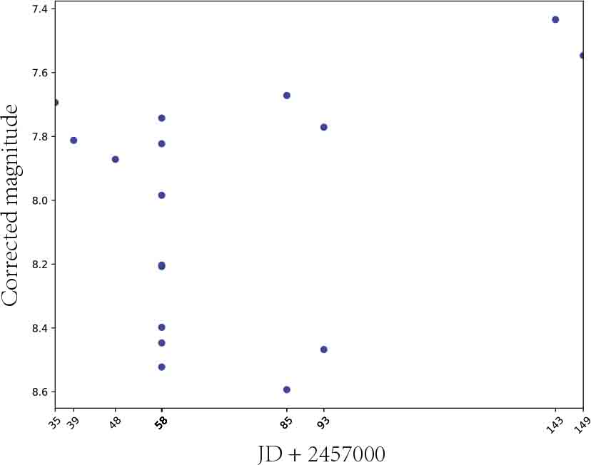
Fig. 8 The light curve of (216) Kleopatra obtained from the Gaia DR2.
Download figure:
Standard imageThe light curve of (216) Kleopatra in Figure 8 seven points lying approximately on a vertical line. These seven points were observed on two consecutive days; i.e., these seven points were collected for one whole rotational period and can be used to search for the rotational period adopting the BGLS-based method. In a series candidate periods obtained by BGLS, the most possible result lies in the range of (2, 3) hours with the minimum of χ2 (cf. Eq. (9)), the periodogram in the range (2, 3) hours is shown in Figure 9. From the plot we can see the probability of point 2.6927 corresponds to 1, so the best-fit rotational period of (216) Kleopatra is finally obtained as 5.3854 hours, which is consistent with the result obtained by Cellino et al. (2009), Cellino et al. (2019) and Pál et al. (2020). Folded light curves are shown in Figure 10.
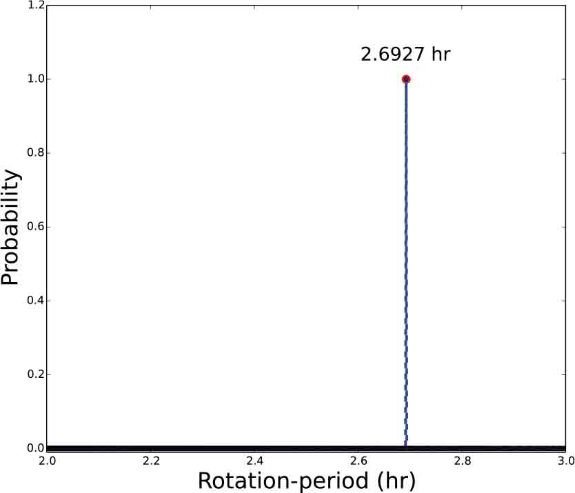
Fig. 9 The periodogram of (216) Kleopatra obtained by BGLS.
Download figure:
Standard image
Fig. 10 Folded light curves for (216) Kleopatra. Red markers are observations calibrated for the phase function while grey light curves are polynomial fitting results.
Download figure:
Standard image6. Conclusions
A BGLS-based method was proposed to search asteroid rotation periods and it was applied to 30 asteroid light curves obtained from the PTF. The rotation periods derived from the BGLS-based method are consistent with that of Waszczak et al. (2015), which suggests that the BGLS-based method is efficient in searching asteroid rotation periods. In addition, this method was applied to a sparse light curve of (216) Kleopatra obtained from the Gaia DR2. The derived rotation period based on the BGLS-method is consistent with the published periods (Cellino et al. 2009, 2019; Pál et al. 2020). Therefore, the proposed method can be applied to the asteroid light curves in the Gaia DR3 in the near future. There is a limitation in the BGLS-based method, that it has not considered the applications for non-principal-axis rotational asteroids. But the research of non-principal-axis rotational periods of asteroids is also important and meaningful, we will pay attention to such issues in subsequent work. A Python code of our BGLS-based method has been published on GitHub 6 , which can be used by the asteroid community.
Acknowledgements
The authors thank Dr. Chan-Kao Chang and anonymous reviewers, whose constructive comments were valuable in strengthening the presentation of this article, and Glenn Pennycook, MSc, from Liwen Bianji, Edanz Group China (www.liwenbianji.cn/ac), for editing the English text of a draft of this manuscript. This work is supported by The Science and Technology Development Fund, Macau SAR (File No. 0158/2019/A3). X.-P. Lu is funded by The Science and Technology Development Fund, Macau SAR (File No. 0073/2019/A2).
Footnotes
- 1
- 2
The range of intervals can be changed depending on the specific requirement. The asteroid rotational periods are not longer than 20 hours and we thus initially search for periods by dividing the period range into 10 intervals (i.e., 1 to 10 hours).
- 3
In this work, K is equal to 12, which is an empirical value.
- 4
- 5
- 6