Abstract
QiTai Telescope (QTT), the world's biggest full-steerable telescope, will be constructed in Xinjiang, China. Its extra high operating frequency (115 GHz) imposes strict requirements on the accuracy of the reflector, while its large aperture (110 m) increases the impact of antenna weight and environment on surface accuracy. However, the panels of reflector will deform under the influence of gravity and the environment. Therefore, to compensate for the performance degradation caused by this deformation, a technique called active surface adjustment has been proposed. The existing adjustment methods cannot detect the deformation caused by environment of the reflector surface in real time, which can result in a delay in the compensation. Consequently, it is difficult to achieve an optimal compensating result. To solve this problem, a real-time method to estimate the large-aperture reflector antenna surface by calculating the antenna panel position based on edge sensors is proposed in this paper. In the proposed method, a panel coordinate transfer matrix has been formulated and the data measured from these edge sensors can then be treated as input for the proposed transfer matrix to calculate the actual position of the antenna panel in real time. A numerical simulation has been carried out in the QTT model and the results obtained show that the proposed real-time method is a promising tool to estimate the large reflector surface position in real time. It is believed that this active surface adjustment method has laid the foundation for new methods that will be developed to compensate for the reflector electrical performance.
Export citation and abstract BibTeX RIS
1. Introduction
Most radio telescopes are designed to be exposed to the natural environment, where gusts of wind and non-uniform temperature distributions can cause the antenna to deviate from its ideal position and can also deteriorate its electrical performance (Rahmat-Samii 1990; Yang et al. 2011; Rajagopalan & Rahmat-Samii 2012). Therefore, it is necessary to adjust the reflector to compensate for the loss of antenna performance in order to improve the gain and pointing accuracy. As high-precision, high-frequency, and large-aperture astronomical telescopes are being developed, the antenna structure is becoming increasingly complex. Moreover, traditional compensation methods can barely meet the electrical performance compensation requirements for large-diameter antennas. To this end, active surface adjustment technologies have been widely used (Zhang et al. 2012; Alvarez et al. 2014; Wang et al. 2017, 2018).
Real-time performance is an important indicator for active surface adjustment technologies, particularly for the QiTai Telescope (QTT), a 110 m full-steerable radio telescope that will be built in China. Rapid adjustment of the actuator can ensure that the telescope can be used effectively. However, the current active surface adjustment method does not meet the real-time performance requirements because of the panel deformation measurement speed. For instance, when the antenna surface is experiencing rapidly varying loads such as wind gusts, it is difficult to detect the reflector panel shape as fast as the load changes. Moreover, calculating the adjustment amount and moving the actuator require additional time; thus, the compensation amount obtained is no longer the required adjustment amount. Therefore, real-time computation of the panel deformation amount is a key problem in active surface adjustment technologies for large-aperture reflector antennas.
The active surface adjustment steps mainly include surface shape detection, appropriate segmentation of main reflector surface, actuator design, active surface control system and surface shape adjustment calculation (Wang et al. 2018). Among these, surface shape detection is the fundamental step in the entire active surface adjustment process. In order to obtain real-time active surface adjustment, the real-time antenna profile measurement must be considered. Since the 1980s, several modern precision measuring instruments have been developed extensively; as a result, the antenna surface detection method has made increasing progress. Consequently, modern measurement methods of the antenna surface shape have seen continuous improvements. As shown in Table 1, commonly used surface shape detection methods mainly include the theodolite method, total station method, photogrammetry, laser tracking measurement, and radio holography (Chen et al. 2016). The first three are optical methods that are primarily used for shape detection and calibration of overall panels before their installation. These measurement methods have the characteristic of large range, high precision, high degree of automation, a tedious process, slow measurement, and dependency on auxiliary equipment; further, they cannot measure reflector surface deformation with the antenna in any pose. Radio holography can be categorized into near-field holography and far-field holography (Bai & Qin 2018). For large-scale radio telescopes, far-field holographic measurement has been widely carried out using celestial bodies or artificial satellites as the source of transmission because of its large range and high precision; however, high measurement accuracy will cause time-consuming (Wang et al. 2018). In addition, although the signal strength of the satellite can be strong enough to ensure high aperture phase resolution, the distribution of artificial satellites is limited and an effective measurement can be only achieved at a certain angle. Thus, the measurement requirements of large radio telescopes cannot be met. The use of near-field holography requires a signal tower and a reference antenna to be set, and, theoretically, this method can satisfy the attitude measurement requirement. However, the construction of signal towers for large radio telescopes is not economical, making field holographic measurements unsuitable in meeting measurement requirements.
Table 1. Surface Measurement Methods Commonly Used in China and Other Countries
| Measurement Method | Characteristic | |
|---|---|---|
| optical method | theodolite method | Large range, high precision, high degree of automation; Tedious process, slow measurement, dependent on auxiliary equipment, limited measurement posture of telescope |
| total station method | ||
| photogrammetry | ||
| radio holography | far-field holography | Large range, high precision; Dependent on other signal sources, limited measurement posture of telescope, expensive auxiliary equipment |
| near-field holography | ||
To overcome the disadvantages of these two types of reflective surface measurement methods, this paper proposes a real-time position calculation method based on an edge sensor. This method can rapidly calculate the actual position of the panels with the antenna at any attitude, which lays the foundation for subsequent calculations of the panel adjustment value.
2. Working Principle of the Edge Sensor
The edge sensor (Mast et al. 1983; Chanan et al. 2004; Shelton et al. 2008) includes two parts, the sensor body and the target (a plane mirror), as shown in Figure 1. The main body is composed of a light-transmitting part, a light-receiving part, and a collimating lens. Light is emitted from the transmitter part and is incident to the plane reflector through the collimating path, which includes a primary mirror and a secondary mirror. After being reflected by the plane reflector, it returns to the receiver part through the same path, as shown in Figure 2. If the sensor body and target are in their standard positions, then the reflected light will return to the center of the receiving part. However, if the position of the plane mirror relative to the sensor body changes, then the spot illuminated by the light deviates from the center position. Therefore, the relative rotation angle can be obtained. The mathematical relationship can be described as Δn = ftan2θ. The experimental prototype accuracy of the edge sensor can reach 0.15".
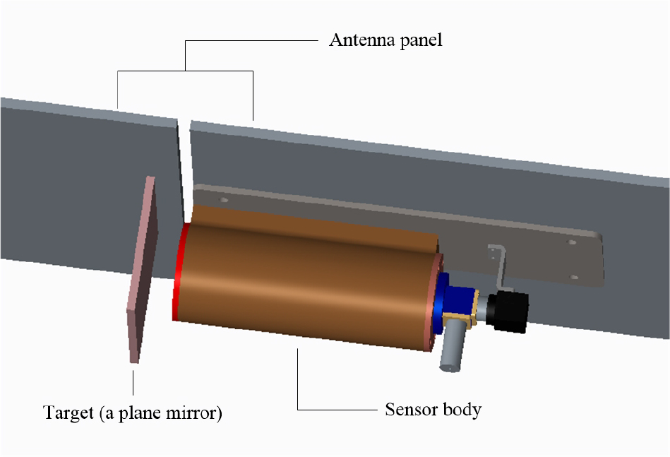
Fig. 1 Structure of the edge sensor.
Download figure:
Standard image
Fig. 2 Working principle of the edge sensor.
Download figure:
Standard image3. Antenna Panel Features and Rotation Matrix
3.1. Panel Partition and Sensor Installation
First, the main girders of the antenna can be categorized into radiating and ring girders. The main reflector panels can be categorized into regions according to the main girders, as shown in Figures 3 and 4. The installation of the edge sensor in every zone can then be determined. Each panel will be installed two edge sensors, as shown in Figure 4. The red line in the figure represents the radiating and ring girders in the zone.

Fig. 3 Overall schematic drawing.
Download figure:
Standard image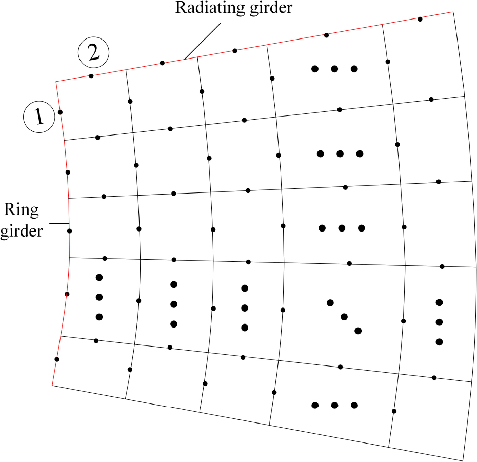
Fig. 4 Enlarged partial view.
Download figure:
Standard imageThe detailed installation principles of the sensor are portrayed in Figure 5. The sensor body is installed on the edge of the adjacent sides of the panel to be tested, and the corresponding matching target is installed on the edge of the adjacent panels. In particular, for panels adjacent to the main girder, the sensor's target can be installed on the radiating or ring girder.
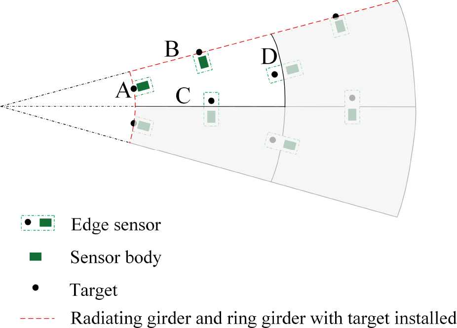
Fig. 5 Specific installation principles of the sensor in one panel.
Download figure:
Standard image3.2. Panel Rotation Transformation Matrix
The measurement principle of the edge sensor is shown in Figure 6. The target (a plane mirror) is installed on a panel, which acts as a reference surface, and the sensor body is installed on an another panel, called panel to be tested. Assume that the panel is rigid and ignore the measurement noise and local deformation of the sensor. When the position of the two panels are relatively changed, the edge sensor measures the inclination of the panel to be measured relative to the reference plane, which is called the rotation angle θ.

Fig. 6 Edge sensor measurement principle.
Download figure:
Standard imageIn a three-dimensional space, the Lodrigues rotation formula can be written as (Yuan et al. 2010)

where ν is a three-dimensional space vector, n 0 is the unit direction vector of the rotation axis, θ is the angle of rotating around ν under the right-hand screw rule, and ν rot is the vector after ν rotation. When the vector in the formula is a row vector, the Lodrigues rotation formula can be rewritten into a matrix form as ν rot = ν R, where

As shown in Figure 7, in the geodetic coordinate system, the ideal coordinates at any point on the panel are set as P(x, y, z); the coordinates after rotation as P(x', y', z'); and the coordinates of a point on the rotation axis as O(a, b, c). The unit direction vector of the rotation axis is n0. The angle of rotation between the two panels is θ.
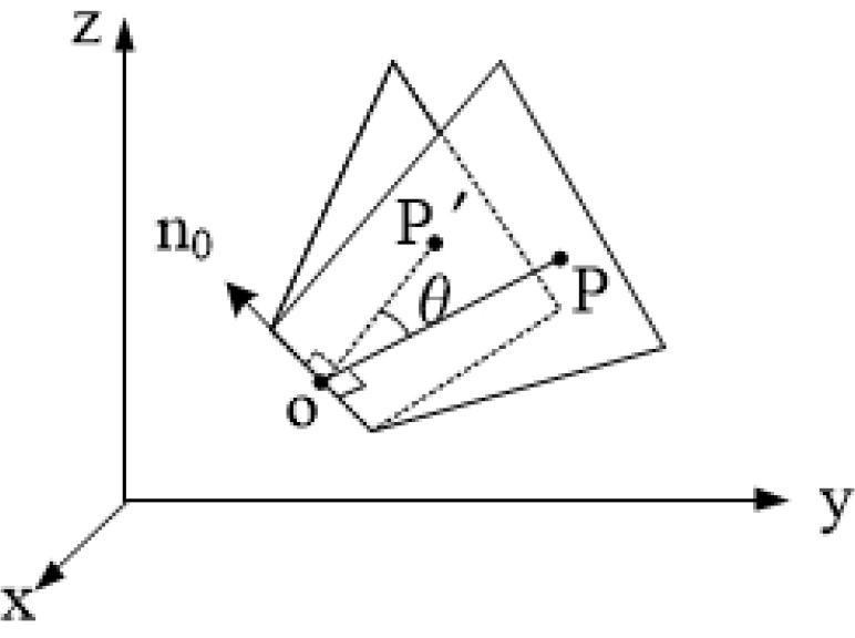
Fig. 7 Rotation matrix calculation diagram.
Download figure:
Standard imageAccording to the Lodrigues rotation formula, the following equation can be deduced: OP ' = OP R. Let the coordinates of point O be (a, b, c,1), those of point P be (x, y, z,1), and those of point P' be (x', y', z',1). Then the formula OP ' = OP R can be transformed into

in which ![$T=\left[\begin{array}{cccc}1 & 0 & 0 & 0\\ 0 & 1 & 0 & 0\\ 0 & 0 & 1 & 0\\ -a & -b & -c & 1\end{array}\right]$](https://content.cld.iop.org/journals/1674-4527/20/11/182/revision2/raa_20_11_182_ieqn1.gif) and
and ![${{\boldsymbol{R}}}_{{\boldsymbol{4}}\times {\boldsymbol{4}}}=\left[\begin{array}{cc}{\boldsymbol{R}} & 0\\ 0 & 1\end{array}\right]$](https://content.cld.iop.org/journals/1674-4527/20/11/182/revision2/raa_20_11_182_ieqn2.gif) . Let
M
=
TR
4 × 4
T
. Therefore, the coordinate transformation relationship between P and P' can be described through a rotation matrix
M
.
. Let
M
=
TR
4 × 4
T
. Therefore, the coordinate transformation relationship between P and P' can be described through a rotation matrix
M
.
4. Panel Position Calculation Method
A region on the antenna panels is first selected assuming that there are M-ring and N-column panels in this region. In the figure, m and n are variables, thus, m ∈ [1, M], n ∈ [1, N]. The numbering rule of the panels can be found in Figure 8.
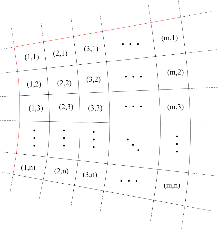
Fig. 8 Panel number.
Download figure:
Standard image4.1. Calculating the Position of the First Panel
Initially, a Cartesian coordinate system with the vertices of the parabolic antenna as the origin was established. Assuming that the edge sensor is installed at the midpoint of the edge of the panel, the coordinates of the node where the edge sensors No. 1 and 2 are located on the first panel can be obtained from the ideal parabolic equation and panel block scheme (Xu & Wang 2016), and the coordinates are set as  and
and  , respectively. According to the working principle of the edge sensor, it is reasonable to assume that the tangent line on the edge of the node where the edge sensor is located is the rotation axis. The direction vector of the rotation axis can be obtained and set as
  and
and  . Let θ11 and φ11 be the angle readings of the two sensors on the first panel, respectively. Based on analysis presented in Section 3.2, the two rotation transformation matrices of the panel (1, 1) can be obtained and set as
M
θ
11
and
M
φ
11
. According to the ideal position coordinates of the panel (1, 1) and its two rotation matrices, the actual position coordinates of any point on the panel (1, 1) can be calculated by
. Let θ11 and φ11 be the angle readings of the two sensors on the first panel, respectively. Based on analysis presented in Section 3.2, the two rotation transformation matrices of the panel (1, 1) can be obtained and set as
M
θ
11
and
M
φ
11
. According to the ideal position coordinates of the panel (1, 1) and its two rotation matrices, the actual position coordinates of any point on the panel (1, 1) can be calculated by

4.2. Calculating the Position of the Panel (m, 1)
When the two sensor targets of a panel are mounted on the radiating girder and panel (m – 1, 1), where the panel number is (m, 1) and m ∈ [2, M]. The ideal coordinates of the nodes where the two sensors are located (the midpoint of the edge of the panel) can then be calculated from the parabolic equation and panel blocking scheme. They can be set as  and
and  . Similarly, assuming that the tangent on the edge of the node where the edge sensor is located (the midpoint of the edge of the panel) is the rotation axis, the direction vector of the rotation axis can be obtained and set as
  and
and  . After obtaining the axis parameters of the rotation matrix, the point parameter
  and
and  can be obtained by
where M θ 11 is the rotation matrix of panel (i, 1) in the θ direction and i ∈ [1, m – 1].
Therefore, the rotation matrix M θ m1 and M φ m1 of panel (m, 1) can be calculated from the obtained axis and point parameters. According to the ideal position coordinates of the panel (m, 1), the actual position of the panel (m – 1, 1), its rotation matrix of the panel (m, 1) and the actual position coordinates of any point on the panel (m, 1) can be calculated by
where xm1, ym1 and zm1 are ideal point coordinates while  ,
,  and
and  are actual point coordinates.
4.3. Calculating the Position of the Panel (1, n)
When the two sensor targets of the panel are mounted on the ring girder and panel (1, n – 1), the panel number is set to (1, n), where n ∈ [2, N]. Similar to the case in Section 4.2, the ideal coordinates of the nodes where the two sensors are located (the midpoint of the edge of the panel) can be calculated from the parabolic equation and the panel blocking scheme. They can be set to  and
and  . Assuming that the tangent on the edge of the node where the edge sensor is located (the midpoint of the edge of the panel) on the rotation axis, the direction vector of the rotation axis can be obtained and set to
  and
and  . After obtaining the axis parameters of the rotation matrix, the point parameters
  and
and  can be obtained by the formula
in which Mφ1j is the rotation matrix of panel (1, j) in the φ direction, where j ∈ [1, n – 1].
Therefore, from the obtained axis and point parameters, the rotation matrices Mθ1n and Mφ1n for panel (1, n) can be calculated. According to the ideal position coordinates of the panel (1, n) the actual position of the panel (1, n – 1) and the rotation matrix of the panel (1, n), the actual position coordinates of any point on the panel (1, n) can be calculated by the formula
where x1n
, y1n
, and z1n
are ideal point coordinates, while  ,
,  ,
,  are actual point coordinates.
4.4. Calculating the Position of the Rest Panel
When the two sensor targets of a panel are mounted on panel (m – 1, n) and panel (m, n – 1), the panel number is set to be (m, n), where m ∈ [2, M] and n ∈ [2, N]. Similar to the previous case, the ideal coordinates of the nodes where the two sensors are located (the midpoint of the edge of the panel) can be determined from the parabolic equation and the panel blocking scheme. They can be set as  and
and  . Assuming that the tangent on the edge of the node where the edge sensor is located (the midpoint of the edge of the panel) is the rotation axis, the direction vector of the rotation axis can be obtained and set as
  and
and  . After obtaining the axis parameters of the rotation matrix, the point parameters
  and
and  can be obtained by the formula
in which Mθin is the rotation matrix of panel (i, n) in the θ direction, where i ∈ [1, m – 1], and Mφmj is the rotation matrix of panel (m, j) in the φ direction, where j ∈ [1, n – 1].
Therefore, from the obtained axis and point parameters, the rotation matrices Mθmn and Mφmn of panel (m, n) can be calculated. According to the actual position of the panel (m – 1, n) and (m, n – 1), the ideal position coordinates of the panel (m, n), and the rotation matrix of the panel (m, n), the actual position coordinates of any point on the panel (m, n) can be calculated by the formula
where xmn
, ymn
, zmn
are ideal point coordinates while  ,
,  ,
,  are actual point coordinates.
5. Numerical Simulation Results
Taking the QTT model as an example for the calculation via simulation, the ratio of f to D is 0.33, the total number of panels is 7168, the total number of rings is 50, and the numbers of columns in each area are 32, 64, 96, and 192 respectively. The panel partitioning scheme and partitioning diagram are shown in Figure 9. The red line in the figure is the boundary of the panel partition, which represents the main radiating girders and ring girders of the antenna.
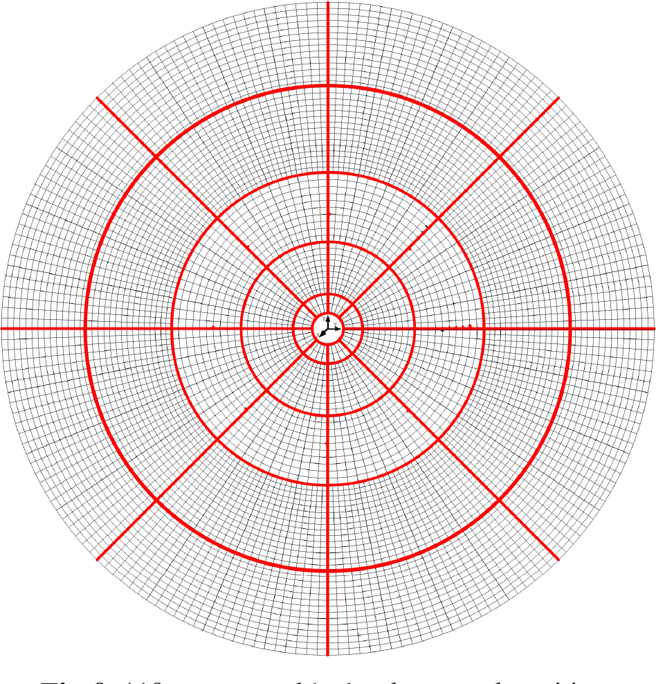
Fig. 9 110 m antenna block scheme and partition.
Download figure:
Standard imageIn this example, a panel area is selected, and the number of panel rings in the area is M=5, whereas the number of panel columns is N=5. The coordinate system used in the calculation is a Cartesian coordinate system with the origin at the apex of the parabolic antenna. The number of endpoints, panels and edge sensors is shown in Figure 10.

Fig. 10 Area panel and sensor number.
Download figure:
Standard imageWith antenna pointing to the sky, we first analyze the distortion of reflector surface under gravity in ANSYS. We then extract the node and sensor information about the target panel area. The antenna FEM model is shown in Figure 11. All of the formulas used in the calculation can be programmed in MATLAB and computed. Finally, we can compare the calculated results with the simulation results to analyze the effectiveness of the proposed method.
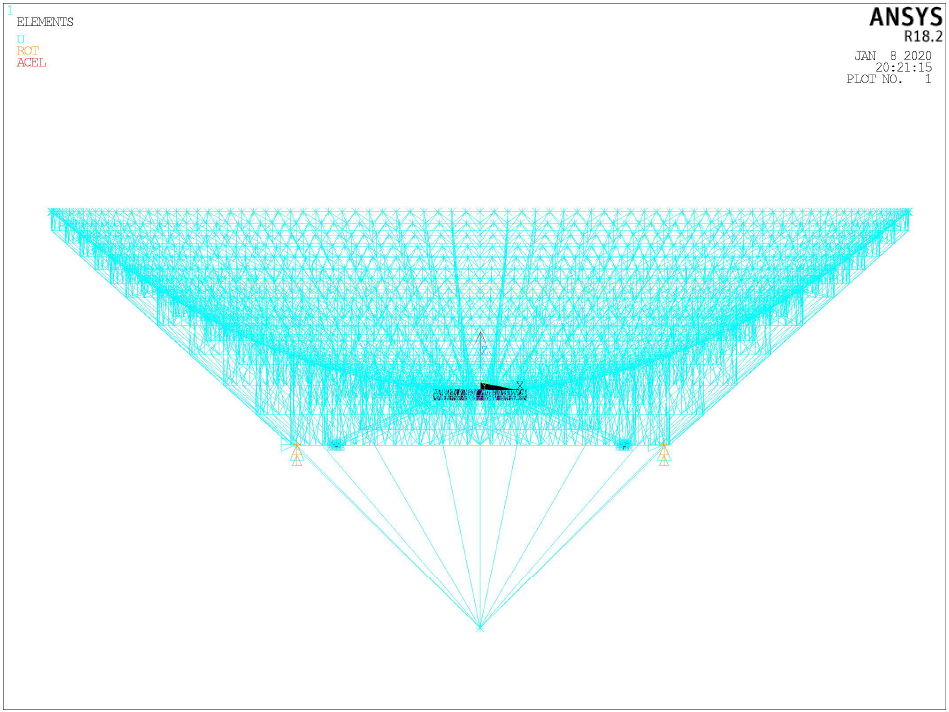
Fig. 11 The 100 m antenna FEM model.
Download figure:
Standard imageTable 2 shows the ideal coordinates of the node located at the position of the edge sensor in target area and the angle values of edge sensor analyzed and computed by the ANSYS and MATLAB. Using the information in Table 2, the position coordinate calculation of each point on each panel can be implemented using MATLAB according to the panel pose calculation process described above. Because this method is finally applied to the active surface adjustment method, it is only necessary to calculate the node coordinates of the installation position of the actuator, that is, the endpoint of each panel, so that we can calculate the movement amount along the normal direction. The ideal endpoint coordinates and deformation endpoint coordinates extracted from ANSYS are shown in Tables 3 and 4. The calculation results of corresponding endpoints is shown in Table 5. The movement amount along the normal direction is shown in Table 6.
Table 2. Ideal Position Coordinates and Computed Value of Edge Sensor
| Coordinates of the edge sensor | Angle of sensor | ||||
|---|---|---|---|---|---|
| Panel number | Sensor number | x/mm | y/mm | z/mm | ° |
| (1,1) | 1 | 5948.67 | 783.16 | 272.73 | 0.01202 |
| 2 | 7154.65 | 468.94 | 389.46 | –0.01203 | |
| (2,1) | 1 | 8268.65 | 1088.59 | 526.94 | 0.0027 |
| 2 | 9484.65 | 621.66 | 684.43 | –0.00932 | |
| (3,1) | 1 | 10578.72 | 1392.71 | 862.49 | 0.00138 |
| 2 | 11829.62 | 775.35 | 1064.70 | –0.00794 | |
| (4,1) | 1 | 12928.44 | 1702.06 | 1288.19 | 0.00194 |
| 2 | 14164.61 | 928.40 | 1526.50 | –0.00601 | |
| (5,1) | 1 | 15218.68 | 2003.58 | 1785.02 | 0.0014 |
| 2 | 16457.19 | 1078.66 | 2060.63 | –0.00473 | |
| (1,2) | 1 | 5795.55 | 1552.91 | 272.73 | 0.01178 |
| 2 | 7032.23 | 1398.80 | 389.46 | 0.00208 | |
| (2,2) | 1 | 8055.82 | 2158.55 | 526.94 | 0.0021 |
| 2 | 9322.36 | 1854.33 | 684.43 | 0.00286 | |
| (3,2) | 1 | 10306.43 | 2761.60 | 862.49 | 0.00154 |
| 2 | 11627.21 | 2312.80 | 1064.70 | 0.00165 | |
| (4,2) | 1 | 12595.67 | 3375.00 | 1288.19 | 0.00335 |
| 2 | 13922.25 | 2769.31 | 1526.50 | 0.00092 | |
| (5,2) | 1 | 14826.96 | 3972.87 | 1785.02 | 0.0056 |
| 2 | 16175.60 | 3217.53 | 2060.63 | 0.00347 | |
| (1,3) | 1 | 5543.28 | 2296.10 | 272.73 | 0.01209 |
| 2 | 6789.49 | 2304.72 | 389.46 | 0.00173 | |
| (2,3) | 1 | 7705.16 | 3191.58 | 526.94 | 0.00264 |
| 2 | 9000.57 | 3055.28 | 684.43 | –0.00008 | |
| (3,3) | 1 | 9857.79 | 4083.23 | 862.49 | 0.00137 |
| 2 | 11225.86 | 3810.66 | 1064.70 | 0.00057 | |
| (4,3) | 1 | 12047.39 | 4990.19 | 1288.19 | 0.00192 |
| 2 | 13441.67 | 4562.83 | 1526.50 | 0.00039 | |
| (5,3) | 1 | 14181.55 | 5874.19 | 1785.02 | 0.00134 |
| 2 | 15617.25 | 5301.34 | 2060.63 | –0.00129 | |
| (1,4) | 1 | 5196.15 | 3000.00 | 272.73 | 0.01173 |
| 2 | 6430.58 | 3171.21 | 389.46 | 0.00183 | |
| (2,4) | 1 | 7222.65 | 4170.00 | 526.94 | 0.00204 |
| 2 | 8524.78 | 4203.95 | 684.43 | 0.00228 | |
| (3,4) | 1 | 9240.49 | 5335.00 | 862.49 | 0.00157 |
| 2 | 10632.43 | 5243.33 | 1064.70 | 0.00144 | |
| (4,4) | 1 | 11292.97 | 6520.00 | 1288.19 | 0.00162 |
| 2 | 12731.11 | 6278.29 | 1526.50 | 0.00172 | |
| (5,4) | 1 | 13293.49 | 7675.00 | 1785.02 | 0.00124 |
| 2 | 14791.67 | 7294.45 | 2060.63 | 0.00009 | |
| (1,5) | 1 | 4760.12 | 3652.57 | 272.73 | 0.01171 |
| 2 | 5961.64 | 3983.44 | 389.46 | 0.00126 | |
| (2,5) | 1 | 6616.57 | 5077.07 | 526.94 | 0.00219 |
| 2 | 7903.12 | 5280.70 | 684.43 | –0.00019 | |
| (3,5) | 1 | 8465.08 | 6495.48 | 862.49 | 0.00102 |
| 2 | 9857.07 | 6586.29 | 1064.70 | 0.00024 | |
| (4,5) | 1 | 10345.33 | 7938.25 | 1288.19 | 0.0029 |
| 2 | 11802.71 | 7886.32 | 1526.50 | –0.00034 | |
| (5,5) | 1 | 12177.97 | 9344.49 | 1785.02 | 0.00494 |
| 2 | 13713.01 | 9162.74 | 2060.63 | 0.00189 | |
Table 3. Ideal Endpoint Coordinates of the Panels
| Number | x/mm | y/mm | z/mm | Number | x/mm | y/mm | z/mm | Number | x/mm | y/mm | z/mm |
|---|---|---|---|---|---|---|---|---|---|---|---|
| 1 | 5987.15 | 392.42 | 272.73 | 13 | 10647.15 | 697.85 | 862.49 | 25 | 15317.13 | 1003.94 | 1785.02 |
| 2 | 5884.71 | 1170.54 | 272.73 | 14 | 10464.98 | 2081.61 | 862.49 | 26 | 15055.05 | 2994.64 | 1785.02 |
| 3 | 5681.58 | 1928.64 | 272.73 | 15 | 10103.74 | 3429.76 | 862.49 | 27 | 14535.38 | 4934.10 | 1785.02 |
| 4 | 5381.24 | 2653.73 | 272.73 | 16 | 9569.63 | 4719.22 | 862.49 | 28 | 13767.00 | 6789.13 | 1785.02 |
| 5 | 4988.82 | 3333.42 | 272.73 | 17 | 8871.78 | 5927.93 | 862.49 | 29 | 12763.06 | 8528.00 | 1785.02 |
| 6 | 4511.04 | 3956.07 | 272.73 | 18 | 8022.13 | 7035.22 | 862.49 | 30 | 11540.74 | 10120.96 | 1785.02 |
| 7 | 8322.14 | 545.46 | 526.94 | 19 | 13012.08 | 852.86 | 1288.19 | 31 | 17597.24 | 1153.38 | 2356.01 |
| 8 | 8179.75 | 1627.05 | 526.94 | 20 | 12789.44 | 2543.98 | 1288.19 | 32 | 17296.15 | 3440.42 | 2356.01 |
| 9 | 7897.40 | 2680.81 | 526.94 | 21 | 12347.97 | 4191.57 | 1288.19 | 33 | 16699.11 | 5668.58 | 2356.01 |
| 10 | 7479.92 | 3688.69 | 526.94 | 22 | 11695.22 | 5767.44 | 1288.19 | 34 | 15816.35 | 7799.76 | 2356.01 |
| 11 | 6934.46 | 4633.46 | 526.94 | 23 | 10842.36 | 7244.64 | 1288.19 | 35 | 14662.97 | 9797.48 | 2356.01 |
| 12 | 6270.34 | 5498.94 | 526.94 | 24 | 9803.99 | 8597.87 | 1288.19 | 36 | 13258.70 | 11627.56 | 2356.01 |
Table 4. Deformation Endpoint Coordinates of the Panels from ANSYS
| Number | x/mm | y/mm | z/mm | Number | x/mm | y/mm | z/mm | Number | x/mm | y/mm | z/mm |
|---|---|---|---|---|---|---|---|---|---|---|---|
| 1 | 5987.26 | 392.46 | 250.87 | 13 | 10647.47 | 697.91 | 839.77 | 25 | 15317.65 | 1004.01 | 1761.75 |
| 2 | 5884.81 | 1170.63 | 250.86 | 14 | 10465.29 | 2081.73 | 839.77 | 26 | 15055.56 | 2994.80 | 1761.79 |
| 3 | 5681.69 | 1928.77 | 250.85 | 15 | 10104.05 | 3429.94 | 839.75 | 27 | 14535.88 | 4934.36 | 1761.72 |
| 4 | 5381.33 | 2653.90 | 250.84 | 16 | 9569.93 | 4719.47 | 839.75 | 28 | 13767.47 | 6789.49 | 1761.70 |
| 5 | 4988.92 | 3333.64 | 250.82 | 17 | 8872.07 | 5928.25 | 839.73 | 29 | 12763.51 | 8528.45 | 1761.71 |
| 6 | 4511.13 | 3956.34 | 250.81 | 18 | 8022.39 | 7035.60 | 839.74 | 30 | 11541.15 | 10121.50 | 1761.65 |
| 7 | 8322.34 | 545.51 | 504.59 | 19 | 13012.50 | 852.92 | 1265.16 | 31 | 17597.86 | 1153.46 | 2332.57 |
| 8 | 8179.95 | 1627.16 | 504.60 | 20 | 12789.86 | 2544.12 | 1265.15 | 32 | 17296.70 | 3440.60 | 2332.84 |
| 9 | 7897.59 | 2680.96 | 504.57 | 21 | 12348.38 | 4191.79 | 1265.13 | 33 | 16699.71 | 5668.89 | 2332.53 |
| 10 | 7480.10 | 3688.90 | 504.57 | 22 | 11695.61 | 5767.74 | 1265.13 | 34 | 15816.92 | 7800.18 | 2332.50 |
| 11 | 6934.63 | 4633.72 | 504.56 | 23 | 10842.74 | 7245.02 | 1265.10 | 35 | 14663.46 | 9797.98 | 2332.69 |
| 12 | 6270.50 | 5499.26 | 504.57 | 24 | 9804.33 | 8598.32 | 1265.09 | 36 | 13259.17 | 11628.18 | 2332.45 |
Table 5. Calculation Results of Corresponding Endpoints
| Number | x/mm | y/mm | z/mm | Number | x/mm | y/mm | z/mm | Number | x/mm | y/mm | z/mm |
|---|---|---|---|---|---|---|---|---|---|---|---|
| 1 | 5987.03 | 392.36 | 250.08 | 13 | 10647.02 | 697.83 | 839.39 | 25 | 15316.72 | 1003.88 | 1761.38 |
| 2 | 5884.69 | 1170.54 | 250.79 | 14 | 10464.82 | 2081.57 | 839.57 | 26 | 15054.61 | 2994.52 | 1761.54 |
| 3 | 5681.55 | 1928.63 | 250.92 | 15 | 10103.56 | 3429.69 | 839.76 | 27 | 14534.91 | 4933.92 | 1761.76 |
| 4 | 5381.19 | 2653.72 | 251.02 | 16 | 9569.44 | 4719.13 | 839.86 | 28 | 13766.54 | 6788.90 | 1761.78 |
| 5 | 4988.77 | 3333.40 | 251.10 | 17 | 8871.59 | 5927.83 | 839.95 | 29 | 12762.61 | 8527.72 | 1761.89 |
| 6 | 4510.98 | 3956.05 | 251.14 | 18 | 8021.92 | 7035.10 | 840.02 | 30 | 11540.27 | 10120.66 | 1761.97 |
| 7 | 8322.09 | 545.45 | 504.15 | 19 | 13011.82 | 852.82 | 1264.74 | 31 | 17596.64 | 1153.30 | 2332.33 |
| 8 | 8179.67 | 1627.04 | 504.38 | 20 | 12789.16 | 2543.91 | 1264.90 | 32 | 17295.47 | 3440.24 | 2332.67 |
| 9 | 7897.30 | 2680.78 | 504.56 | 21 | 12347.66 | 4191.46 | 1265.16 | 33 | 16698.49 | 5668.34 | 2332.56 |
| 10 | 7479.81 | 3688.65 | 504.71 | 22 | 11694.91 | 5767.29 | 1265.23 | 34 | 15815.77 | 7799.45 | 2332.48 |
| 11 | 6934.34 | 4633.41 | 504.80 | 23 | 10842.05 | 7244.45 | 1265.32 | 35 | 14662.37 | 9797.07 | 2332.77 |
| 12 | 6270.22 | 5498.88 | 504.86 | 24 | 9803.66 | 8597.67 | 1265.41 | 36 | 13258.09 | 11627.15 | 2332.77 |
Table 6. Movement Amount along the Normal Direction
| Number | Movement amount/mm | Number | Movement amount/mm | Number | Movement amount/mm |
|---|---|---|---|---|---|
| 1 | 0.566 | 13 | 1.097 | 25 | 2.504 |
| 2 | –0.161 | 14 | –1.280 | 26 | 2.669 |
| 3 | –0.291 | 15 | –1.472 | 27 | 2.894 |
| 4 | 0.393 | 16 | 1.574 | 28 | 2.915 |
| 5 | 0.473 | 17 | 1.663 | 29 | 3.026 |
| 6 | 0.513 | 18 | 1.736 | 30 | 3.110 |
| 7 | –0.482 | 19 | 1.769 | 31 | 3.296 |
| 8 | 0.714 | 20 | 1.931 | 32 | 3.648 |
| 9 | –0.896 | 21 | 2.194 | 33 | 3.533 |
| 10 | 1.046 | 22 | 2.266 | 34 | 3.453 |
| 11 | 1.137 | 23 | 2.358 | 35 | 3.751 |
| 12 | 1.197 | 24 | 2.450 | 36 | 3.752 |
In this study, 36 points were selected, and the total calculation time was 9.9s. Besides, there are 3168 nodes in the whole reflector surface of the antenna model in this article, which are divided into 32 areas, a total of four categories, each category has 36, 72, 144, 144 nodes. According to the simulation results, the calculation time for the 36-node area is 9.9s, the calculation time for the 72-node area is 10.3s, and the calculation time for the 144-node area is 11.8s. (OS: Windows 10, CPU: Intel (R) Core (TM) i5-8500 CPU of 3.00GHz, Memory: 16GB). Then, simulate all nodes. If the calculation of all areas is a serial computing, that is, the next area is calculated after one area is calculated, the total calculation time is about 1400s, a total of 24min. If the calculation of all regions is parallel computing, — that is, the calculation of each area is calculated at the same time — then the total calculation time is about 12s. In practical applications, the calculation process in each area should be performed simultaneously; thus, for the 110m antenna, the calculation method has, to some extent, satisfied the real-time performance requirements.
6. Conclusions
In this paper, a real-time calculation method for the QTT panel position based on edge sensor has been proposed. The angle position measured by the edge sensor and ideal position of the antenna panel is used to calculate the actual position of the panel after deformation, and the numerical simulation of the method is performed in ANSYS and MATLAB. From the perspective of calculation time, the method has satisfied real-time performance requirements; thus, it can be used to guide the subsequent active adjustment of the surface shape of QTT and further compensate the electrical performance of the large-diameter reflector antenna to achieve better technical specifications. Simultaneously, the use of edge sensors will also increase the weight of the antenna. Therefore, in future work, experiments under the influence of sensor weights can be continued to verify the measurement accuracy of the method. In addition, we can continue to study the calculation efficiency and accuracy of this method. Besides, the adjustment accuracy and execution speed of the adjustment mechanism of the panel, that is, the actuator, will also affect the observation performance of the reflector antenna. Considering the actual situation, there is a certain error in the amount of movement of the actuator. The concept of interval analysis can also be introduced into our proposed method.
Acknowledgements
This work was supported by the National Natural Science Foundation of China (Nos. 51975447, U1737211 and 51805399), the Natural Science Foundation of Shaanxi Province (No. 2018JZ5001), the Youth Innovation Team of Shaanxi Universities (No. 201926), and the Tianshan Innovation Team Plan (No. 2018D14008).