Abstract
The Five-hundred-meter Aperture Spherical radio Telescope (FAST) has the potential to discover many new pulsars and new phenomena. In this paper we mainly concentrate on how FAST can impact study of the pulsar emission mechanism and magnetospheric dynamics. Several observational programs heading to this direction are reviewed. To make full use of the superior performance of FAST and maximize the scientific outcome, these programs can be arranged in different phases of FAST according to their demands for observational conditions. We suggest that programs can be performed following the test phase, which are observations of multifrequency mean pulse profiles, anomalous X-ray pulsars (AXPs)/soft gamma-ray repeaters (SGRs), mode changing, drifting subpulse and nulling. The long-term monitoring can be carried out for mode changing, AXPs/SGRs and precessional pulsars. Others programs, including polarization observations of radio and γ-ray pulsars, searching for weak pulse components, and multifrequency observations of subpulse drifting, microstructure and giant pulses, can be conducted in all the normal operating phases (the first and second phases). These programs will push forward the frontier in this field in different respects. The search for sub-millisecond pulsars and follow-up observations of their emission properties are very important projects for FAST, but they may be covered by other papers in this mini-volume; therefore, they are not discussed here.
Export citation and abstract BibTeX RIS
1. Introduction
With superior sensitivity compared to any other single-dish radio telescope, it is promising to discover more new pulsars and new pulsar phenomena with the Five-hundred-meter Aperture Spherical radio Telescope (FAST) (Zhang et al. 2016). Since its first light in September 2016, more than 20 new pulsars have been discovered during the phase of commissioning, already showing the power of this facility. The pulsar community is now facing a question: what kinds of observing programs should be proposed so as to make full use of FAST and promote deeper understanding of the physics of pulsars, gravitational waves, interstellar medium, Galactic magnetic field, etc. In this paper, we mainly focus on the emission mechanism, an old problem in pulsar studies, in which FAST may shed new insights. We will look ahead to related programs that can be performed in different stages of FAST.
Over the past five decades, it has been widely accepted that the associated coherent radio emission is generated by secondary relativistic particles, which are produced via the pair production process in and out of the gaps in the open field line region of a pulsar magnetosphere. Several candidate mechanisms have been proposed, e.g. curvature radiation (e.g. Sturrock 1971; Ruderman & Sutherland 1975), curvature maser emission (Beskin et al. 1988), inverse Compton scattering (hereafter ICS, Qiao 1988; Qiao & Lin 1998; Xu et al. 2000; Qiao et al. 2001; Lee et al. 2009; Lv et al. 2011) and maser linear acceleration emission (Melrose et al. 2009; Melrose & Luo 2009 among which the ICS model is the most adaptable to account for various properties of the mean pulse profile and polarization. However, the radio emission mechanism is still an open question. A vital route to test emission models is to compare the model predictions on the frequency dependence of pulse profile and polarization for a large sample of pulsars. Unfortunately, at present such kind of sample is still very limited.
For example, in a recent census on the frequency evolution of pulse width, Chen & Wang (2014) could only collect a sample of ∼150 pulsars with relatively good-quality profiles within a frequency range over a factor of three from the European Pulsar Network (EPN), so far the only public multifrequency profile database containing about a half of the currently known pulsars.
It is believed that the observed single pulse properties, e.g. flux density modulation, microstructure, nulling and subpulse drifting, are related to stochastic or periodic processes in particle emission or/and dynamics. Although the mean pulse profile is stable for most pulsars, a small percentage of pulsars does show the phenomenon of strikingly quasi-periodic (e.g. Lyne et al. 2010) or random (e.g. Chen et al. 2011) profile changes, which is conventionally called mode changing or mode switching (Backer 1970). Some recent efforts have been undertaken to understand a large variety of mode switching phenomena, i.e. nulling, subpulse drifting, profile mode changing and some extreme cases like intermittent pulsars (e.g. Kramer et al. 2006) and rotating radio transients (RRATs) (e.g. McLaughlin et al. 2006), in a more general way. However, there are no self-consistent models yet. Again, an important reason is that the samples of pulsars with those phenomena are still very small compared with the total number of known pulsars because of the limitations of observing sensitivity and time.
We present several topics in the following sections: multifrequency observations of mean pulse profiles and polarizations in Section 2, single-pulse observations in Section 3, special phenomena in Section 4 and then discuss arrangement of the observing programs in different phases of FAST in Section 5. The concluding remarks are made in Section 6.
2. Observations of the mean pulse profile and polarization
2.1. Multifrequency Mean Pulse Profiles
The planned observing frequency will cover the range 70 MHz∼3 GHz. With a much larger sky coverage and a factor of 3 better raw sensitivity compared with Arecibo (Nan et al. 2011), FAST will provide us a larger sample of multifrequency profiles with high signal-to-noise ratio (S/N). Below is a simple estimation of the scale of the samples of different S/N levels based on known pulsars archived in the ATNF Pulsar Catalogue (Manchester et al. 2005).1
The S/N of pulse peak for an integration time tint can be calculated with the following equation (Dewey et al. 1985)

where S is the flux density of a pulsar, Tsys and Tsky are the system temperature (K) and the sky temperature (K), respectively, G is the telescope gain, P is the pulsar period (s), np is the number of polarizations, Δf is the observation bandwidth (MHz) and W is the equivalent pulse width (s). The sky temperature differs at different bands. Taking L-band as an example, the sky temperature is usually within 10–20 K on the Galactic plane and negligible outside. Here we simply assume Tsky = 15 K for |b| ≤ 5 ° and Tsky = 4 K for |b| > 5 °.2
In principle, the S/N can be computed for all the 1187 known pulsars located in the FAST zone within the declination range of −15 ° < δ < +65°. Unfortunately, only 910 pulsars have enough information on pulse width and flux density for this calculation. Lacking data on equivalent width, we use the full width at half maximum, Wa50, downloaded from the ATNF Pulsar Catalogue, instead. When W50 is not available, half of the 10% pulse width (W10/2) is used. When both of them are absent, the pulse duty cycle is assumed to be 5%. The Smin is replaced by the archived L-band flux density S1400. When there are no S1400 data, S1400 values are extrapolated from the S400 data, if possible, with a power law assuming a spectral index of −2. For a one-hour observation (tint = 1h) at L-band with

and Δf = 400 MHz3, the number of all pulsars in the visible zone, Ninz, the number of pulsars with S1400 data, Nflx, and the expected numbers of pulsars with S/N≥ 100, 1000, 10 000, as denoted by N100+, N1000+ and N10 000+, respectively, are calculated. The same method is applied to the Arecibo and Parkes telescopes using their own parameters: Tsys = 24 K, G = 10 K Jy−1, np = 2, Δf = 300 MHz and −1 ° < δ < +38 ° for Arecibo (Cordes et al. 2006); Tsys = 28 K, G = 0.8 K Jy−1, np = 2, Δf = 256 MHz and −90 ° < δ < +27 ° for Parkes (Hobbs et al. 2019).
We are aware that some other factors may induce uncertainties in the S/N, e.g. the oversimplification of Tsky and equivalent pulse width, radio frequency interference, interstellar scintillation, etc., and hence affect the above estimation. In order to test the validity, we compared the theoretical S/N with the observed S/N for 600 pulsars discovered in the Parkes Multibeam Pulsar Survey (Manchester et al. 2001; Morris et al. 2002; Kramer et al. 2003; Hobbs et al. 2004). Because the integration time is 2100 s in the detection, the published S/N values are multiplied by a factor of 1.3 to coincide with an integration time of 1 h. The theoretical S/N values are found to be 2.0±1.3 times the observed values, resulting in an overestimation of the predicted N100+ by a factor of 4.5 with respect to the observed N100+ (112:25). But as for the number of pulsars with S/N> 40, the factor decreases to 2.3 (355:155). Therefore, we use a practical factor of 3 to correct the predicted sample numbers. All the numbers of N100+, N1000+ and N10 000+ are divided by 3, assuming that this factor also applies to FAST and Arecibo. The final results are listed in Table 1 for comparison. Although uncertainties still exist, the great capability of FAST in enlarging the high-S/N samples is evident.
Table 1. Expected Numbers of Samples with High S/N for 1 h Observations at L-band
| Telescope | Ninz | Nflx | N100+ | N1000+ | N10 000+ |
|---|---|---|---|---|---|
| FAST | 1187 | 910 | 294 | 202 | 41 |
| Arecibo | 697 | 535 | 165 | 66 | 10 |
| Parkes | 2338 | 1824 | 204 | 23 | 2 |
The current emission models have different predictions on the frequency evolution of mean pulse profiles. For example, the curvature radiation models predict that the beam radius and pulse width decrease with increasing frequency (e.g. (e.g. Ruderman & Sutherland 1975; Gil & Snakowski 1990; Wang et al. 2013). The ICS model predicts two types of "beam radius-to-frequency mapping." For type I, the beam consists of a core and an inner hollow cone, where the radius of the core decreases slightly with increasing frequency while that of the inner cone increases with frequency. For type II, besides those two components, the beam has an additional outer hollow cone, the radius of which decreases with increasing frequency (Qiao & Lin 1998; Qiao et al. 2001). Therefore, the ICS model is more adaptable for explaining various kinds of frequency development of pulse width and pulse shape. Although most of the emission models have a long history, observational tests and constraints on model parameters have been done for less than 20 pulsars (Zhang et al. 2007; Lee et al. 2009; Lv et al. 2011; Wang et al. 2013). With a sample of 150 pulsars selected from the EPN database, Chen & Wang (2014) measured the relative fraction of pulse width change between 0.4 GHz and 4.85 GHz, i.e. η = (W4.85 − W0.4)/W0.4, where W is the pulse width at the level of 10% of the pulse peak. It is found that 54% of the pulsars have η < −10, showing considerable profile narrowing at high frequency, 27% have −10%≤ η ≤ 10%, exhibiting either a small positive or negative change in pulse width and 19% have η > 10%, showing remarkable profile broadening. Such a large fraction of the latter two cases4 suggests that the models that can only predict the profile narrowing at high frequency are unlikely to be the general emission model for radio pulsars. However, these efforts revealed only the tip of the iceberg. Observing programs need to be performed with FAST to provide a larger sample of pulsars with high S/N profiles, especially at high frequencies, to enable more comprehensive understanding of frequency evolution of pulse profiles and further test models.
The future observations will be also helpful for testing narrowband and broadband emission models. The core-conal beam model (Rankin 1983) is a popular empirical model that assumes emission at a single altitude is narrowband. Incorporating with the radius-to-frequency mapping (RFM), i.e. lower frequency emission comes from higher altitude, this model predicts shrinkage of the pulse profile with increasing frequency. For a broadband emission model, e.g. the fan beam model (Wang et al. 2014), since the emission at a single altitude is broadband, it predicts that there should be multifrequency emission at any phase within the whole pulse window, even though the high-frequency emission may be very weak near the edge of a pulse window for the pulsars that exhibit the profile narrowing phenomenon. These predictions can be tested by checking whether there is weak and extended emission outside the previously determined pulse window when the S/N is improved at high frequency in the future. But owing to the power-law spectra of pulsars and limited observing time, the S/Ns of the published high-frequency profiles are not comparable to those at lower frequencies for many pulsars. FAST is very useful for overcoming this selection effect, making it possible to perform this kind of test. Furthermore, the time-aligned multifrequency profiles can be used to study the spatial distribution of the emission spectrum in a pulsar magnetosphere(Lyne & Manchester 1988; Kramer et al. 1994; Chen et al. 2007; Dai et al. 2015)
2.2. Polarization of Normal Pulsars
High-quality polarization observations will be useful for probing the structure of a radio beam. The core-conal beam model (Rankin 1983) and patchy beam model (Lyne & Manchester 1988) have posed a long-term debate on the beam structure of radio pulsars, where the former proposed that a typical radio beam consists of two nested cones and a central core, while the latter argued that the intensity distribution is random and patchy within the beam. In spite of this difference, they have a common assumption that the beam has a circular or elliptical boundary, outside of which the emission is negligible. Such an assumption predicts that one would see a narrower pulse width if the line of sight sweeps across the beam from a further place with respect to the magnetic pole. However, Wang et al. (2014) found an opposite trend, namely, a positive correlation between the pulse width and the impact angle by collecting a sample of 64 pulsars, among which the impact angle between our line of sight and the magnetic pole was constrained through fitting the linear polarization position angle (hereafter PPA) data with the rotating vector model (RVM, Radhakrishnan & Cooke 1969). This trend, together with the other three pieces of evidence, was found to be generally consistent with the prediction of the fan beam model proposed by them, in which the beam consists of a few fan-like sub-beams.
FAST will provide a larger sample of normal pulsars with the impact and inclination angles constrained with the RVM-fitting method. On one hand, more pulsars with an "S"-shaped PPA curve could be found, and on the other hand, the observations with high S/N of previously known pulsars with an "S"-shaped PPA curve will extend the pulse phase window where the PPA can be measured and hence reduce the uncertainties in the constrained inclination and impact angles. An improved sample will enable us to perform {a }further test for the radio beam structure and map the geometry of the emission region.
2.3. Polarization of Gamma-ray Pulsars
Combining pulse profiles with the inclination and impact angles constrained with the RVM-fitting method, the geometry of radio and gamma-ray emission regions of pulsars can be constrained more reliably than through only fitting the radio and gamma-ray pulse profiles and their phase offset with radio and gamma-ray emission models. Such a joint fitting technique has been successfully applied to the gamma-ray pulsar PSR B1055-52 (Wang et al. 2006; Weltevrede & Wright 2009). At present, the latter method (profile fitting) is widely used to constrain the emission geometry of gamma-ray millisecond and normal pulsars (e.g. Johnson et al. 2014; Pierbattista et al. 2015), however, the resultant inclination angles of young Fermi pulsars (Pierbattista et al. 2015) are statistically much larger than those constrained with the RVM-fitting method (Rookyard et al. 2015a,b with the Parkes radio telescope). FAST can hopefully provide a larger sample of gamma-ray pulsars with the viewing geometry constrained by the RVM method. In particular, the extended longitude range revealed by deep observations may help in reducing the uncertainty in estimation of inclination angle, which will enable application of the joint fitting technique to more gamma-ray pulsars.
In principle it can also be applied to gamma-ray millisecond pulsars (MSPs). Although the PPA curves of MSPs are normally complex, there is still a small fraction of MSPs with an "S"-shaped PPA curve (Xilouris et al. 1998; Yan et al. 2011).
Table 2 lists the candidates of gamma-ray MSPs with weak radio emission at 1.4 GHz, the PPA curve of which can be generated with FAST. The expected integration time tint needed to acquire an S/N of 1000 is calculated by using Equation (1),assuming a duty cycle of 10% and a factor of 3 to correct the possible overestimation of the predicted S/N. The results are given in the last column in units of hours.
The better constraints on radio and gamma-ray emission regions will be valuable for testing gamma-ray emission models, e.g. the outer gap model (Cheng et al. 1986a,b), the polar gapmodel (Muslimov & Harding 2003) and the annular gap model (Qiao et al. 2004a,b; Du et al. 2010; Du et al. 2011; Du et al. 2012; Du et al. 2013).
Table 2. Gamma-ray MSP Candidates for Polarization Observations
| Name | RA | Dec | l | b | P | S1400 | tint |
|---|---|---|---|---|---|---|---|
| PSR | (h:m:s) | (d:m:s) | (deg) | (deg) | (ms) | (mJy) | (h) |
| J0030+0451 | 00:30:27.4 | +04:51:39.7 | 113.141 | –57.611 | 4.87 | 0.6 | 1.8 |
| J0218+4232 | 02:18:06.3 | +42:32:17.3 | 139.508 | –17.527 | 2.32 | 0.9 | 0.8 |
| J1741+1351 | 17:41:37 | +13:51:4 | 37.896 | 21.619 | 3.75 | 0.93 | 0.8 |
| B1957+20 | 19:59:36.7 | +20:48:15.1 | 59.197 | –4.697 | 1.61 | 0.4 | 8.8 |
| J2017+0603 | 20:17:22.7 | +06:03:05.5 | 48.621 | –16.026 | 2.90 | 0.5 | 2.6 |
2.4. Searching for Weak Pulse Components
Only a few normal pulsars are known to have pre- or postcursors, the components preceding or succeeding the main pulse respectively (Campbell & Heiles 1970; Fowler et al. 1981; Mitra & Rankin 2011), or off-pulse emission (Basu et al. 2011). Some of the precursors and postcursors are weak. In contrast, more and more MSPs have been discovered to have weak pulse components when the observing sensitivity is improved because of a large amount of integration time (Yan et al. 2011, Dai et al. 2015). Most of the known weak components were discovered with single-dish telescopes. They have posed a great challenge to the current emission models. Since FAST is expected to obtain the mean pulse profiles with S/N > 100 for hundreds of pulsars (see Table 1), it is promising to discover new weak components with FAST for normal pulsars and MSPs. It would be interesting to test whether some new models, e.g. the induced Compton scattering model (Petrova 2009) and the fan beam model (Wang et al. 2014), are capable of explaining this phenomenon.
3. Single pulse observations
FAST is expected to record single pulses for more pulsars, as can be seen from the following comparison of the numbers of single-pulse candidates for FAST, Arecibo and the Parkes telescope. Substituting tint = P and the parameters used in Section 2.1 into Equation (1), the Smin for single pulses at a given S/N can be derived. The single-pulse candidates are then selected by using the criterion of S1400 ≥ Smin. For the 910 pulsars with S1400 data in the FAST zone, the number of candidates varies from 741 to 454 when the S/N increases from 5 to 20, as indicated by the solid line in Figure 1. The same method is applied to the Arecibo and Parkes telescopes. Their candidate number-S/N curves are presented by the dashed and dot-dashed lines, respectively. The percentages of candidates to the total samples in each telescope zone (Ninz in Table 1 are also marked for a set of S/N values. Note that the expected number of pulsars that can be observed with Arecibo and the Parkes telescope at the single-pulse S/N of 5 is roughly consistent with the total number of known pulsars with the subpulse drifting and nulling phenomena (< 300). Apparently, FAST will hopefully double the number of pulsars with single pulse detection.
With the superior capability of single pulse detection, FAST may be helpful for answering several important questions relevant to emission mechanisms and dynamics, among which the most interesting one is: are the profile mode changing, nulling, intermittent pulsars, RRATs and other mode-switching phenomena different manifestations of the same physics process? At present, the sample of each phenomenon only occupies a small percentage of known pulsars, but a considerable fraction of the samples is overlapped, namely, a portion of pulsars shows a combination of the profile mode changing, subpulse drifting and even nulling. Larger samples may reveal a clearer link and lead to better classifications. Some topics are discussed further below.
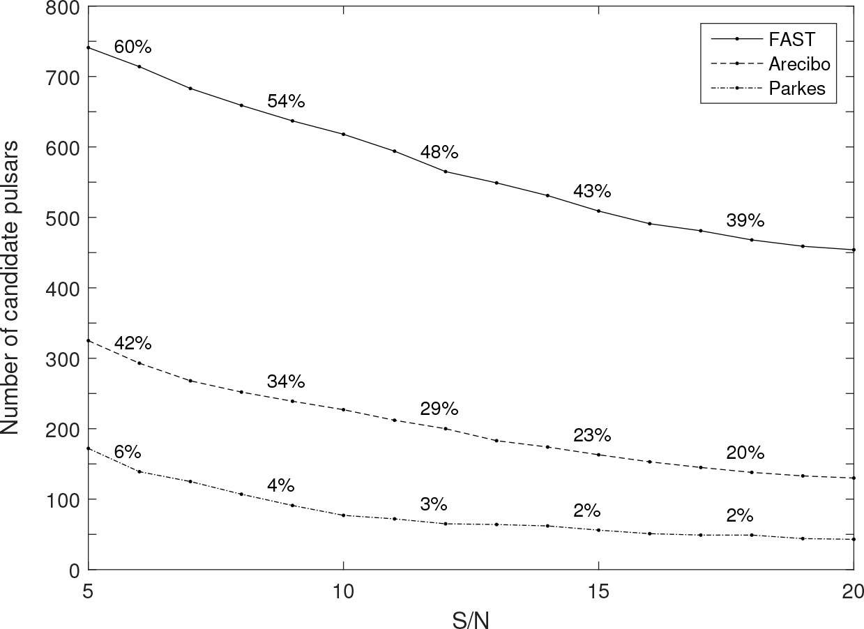
Fig. 1 Number of single-pulse candidates versus S/N required for a single pulse detection. The solid, dashed and dot-dashed lines are for FAST, Arecibo and the Parkes telescope respectively. The number of candidates is estimated by using the criterion: the L-band flux density S1400 must exceed the minimum detectable flux density Smin for an observation time of one pulse period at a given S/N; see text for details of the calculation. Totals of 1187, 697 and 2338 known pulsars are located in the visible zones of the three telescopes, respectively, but only 910, 535 and 1824 of them have S1400 data, from which the candidates are selected. The fractions above the lines represent the percentages of candidates that can reach S/N = 6, 9, 12, 15 and 18 to the total visible samples for each telescope.
Download figure:
Standard image3.1. Mode Changing
A striking phenomenon of mode changing pulsars is that they switch between two or more sets of multifrequency mean pulse profiles. The frequency dependence of pulse profiles suggests that the spectrum across the pulse phase (phase-resolved spectrum) changes when the pulsar switches to another mode, meanwhile, the polarization properties usually change as well (e.g. Bartel et al. 1982; Smith et al. 2013). Single pulse observation with FAST will let us know more important features of mode changing, e.g. how the phase-resolved flux density distribution of single pulses and the single pulse polarization change with mode.
The synchronous observation at radio and X-ray bands is key to understanding how modes are correlated with some physical parameters, e.g. the polar cap surface temperature. Using XMM-Newton, LOFAR and GMRT, Hermsen et al. (2013) discovered an interesting correlation between the radio mode switching ("bright" and "quiet" modes) and the X-ray mode switching (non-thermal and thermal-plus-non-thermal spectra) for PSR B0943+10. However, there is no significant evidence for simultaneous X-ray-radio mode-switching in another pulsar, PSR B1822–09 (Hermsen et al. 2017). More campaigns of simultaneous observations with X-ray and radio telescopes, including FAST and other large radio telescopes, are worth performing to check such kind of correlation for more pulsars. Furthermore, simultaneous observations of radio and X-ray polarizations with FAST and the Hard X-ray Modulation Telescope (HXMT) can be used to diagnose whether the mode switching is correlated with global transformation of the magnetic field structure.
3.2. Nulling
About 190 pulsars are known so far to exhibit nulling (Yang et al. 2014, Basu et al. 2017). The nulling fractions, viz. the percentage of time for nulling, vary from close to 0 to nearly 1.
Only weak correlations were found between the nulling fraction and the pulsar parameters, e.g. pulse period, W50 and characteristic age τ (see Yang 2014 and references therein). Another parameter, the nulling scale, which is defined as the effective length of the consecutive nulling and bursting periods, was reported to be strongly correlated to the derivative of rotation frequency and the loss rate of rotational energy Edot based on an analysis of ten pulsars (Yang et al. 2014).
Is the present sample of nulling pulsars good enough to be free from selection effects? Using the data of 195 nulling pulsars collected by Yang (2014) and Basu et al. (2017), we reproduced a histogram of the nulling fractions in a slightly different way, as shown in Figure 2.. A sharp decline can be seen between the fractions 5% and 20%, but it is not clear whether this feature is intrinsic or caused by selection effects.
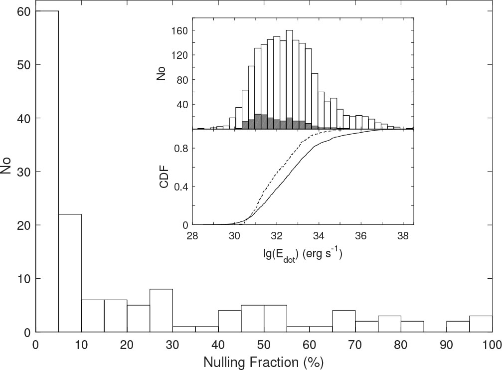
Fig. 2 Histogram of the nulling fraction for 141 pulsars. The top panel of the inset shows the histograms of the rotational energy loss rate Edot for 1913 normal pulsars (white) and the 195 nulling pulsars currently known (dark). The bottom panel presents the empirical CDF for these two samples (the dashed line is for nulling pulsars and the solid line is for normal pulsars). Data are adopted from (2014) and Basu et al. (2017).
Download figure:
Standard imageAnother interesting issue is the relationship between the nulling pulsars and other populations. Since all the nulling pulsars are normal pulsars, we compared the distributions of the surface magnetic fields Bs, τ and Edot for the nulling pulsars and all the normal pulsars. Using the criteria of P > 0.015 s and Bs > 1010 G, 1913 normal pulsars were selected from the ATNF Pulsar Catalogue. The Kolmogorov–Smirnov tests reject the null hypotheses that the two samples come from the same distribution for both Edot and τ at the 5% significance level (with probabilities of 1.6×10⁻⁵ and 5.0×10⁻⁴ assuming that the null hypothesis is true, respectively), but cannot reject the hypothesis that they have the same Bs distribution (with a probability of 0.15). For example, the histograms of Edot for the normal pulsars (white) and the nulling pulsars (dark) are displayed in the top panel of the inset. The difference in the distributions suggests that pulsars with low Edot values seem to have relatively high probability to exhibit nulling, which can also be seen in the empirical cumulative distribution function (CDF) in the bottom panel. Note that Edot∝ Δ V2, where Δ V is the maximum potential drop between the magnetic pole and the edge of the polar cap; therefore, this difference does have some physical implication on the mechanism of nulling. However, the histogram presents a significant decline in the fraction of nulling pulsars in the bins with the lowest Edot (< 2 ∝ 1030 erg s−1), which does not follow the trend. Because S1400 is below 1 mJy for most of these low-Edot pulsars, the selection effect due to telescope sensitivity may have biased the observed distribution.
Among the 22 pulsars with Edot < 2 × 1030 erg s−1 in the FAST zone, 17 sources have S1400 data. It is found that 13 of them may reach an S/N of 9 for single pulses. Compared with 7 out of 11 pulsars that can reach the S/N for Arecibo and 1 out of 41 for the Parkes telescope, FAST will be helpful in reducing the selection effect. A larger sample will benefit study of the timescales of nulling, the classification of nulling patterns (e.g. random or quasi-periodic) and the relationship between the nulling population and other populations. The deep integration over the nulling periods will reveal whether the nulling is due to the ceasing of emission or actually very weak emission.
3.3. Subpulse Drifting
The subpulse drifting phenomenon, firstly discovered by Drake & Craft (1968), is vital to study the electrodynamic process in a pulsar magnetosphere (Ruderman & Sutherland 1975; Gil & Sendyk 2000). A bit more than 100 pulsars are known to show the drifting phenomenon (Gil et al. 2006). In the L-band subpulse-drifting survey performed with the Westerbork Synthesis Radio Telescope (WSRT), 187 pulsars, which have predicted S/N exceeding 130 (computed with Equation (1)) for a 0.5 h observation or a longer time for more than 1000 pulse periods for slow pulsars, were selected to form an unbiased sample. Finally, 106 of them have an observed S/N > 100. In general, it was found that the fraction of drifters is likely to be larger than 55% (Weltevrede et al. 2006). However, the probability of detecting drifting strongly depends on the S/N, which is higher for observations with a higher S/N. On the basis of a sample of 68 drifters, it was found that the drifting phenomenon is more likely to occur in old pulsars, but the period at which a pattern of pulses crosses the pulse window, P3, and the drift direction are not significantly correlated with other pulsar parameters, e.g. the pulsar age and the surface magnetic field strength. Weltevrede et al. (2006) stated that their observations could not rule out different emission models.
Table 3. Magnetars with Radio Emission, High-B Radio Pulsars with X-ray Emission and Anti-magnetars
| Name | P (s) |  (s s−1) (s s−1) |
Bs(G) | Notes |
|---|---|---|---|---|
| Magnetars with radio emission | ||||
| XTE J1810–197 | 5.54 | 7.77 ×10⁻¹² | 2.1 × 10¹⁴ | optical/near infrared, radio(1) |
| SGR J1745–2900 | 3.76 | 1.39 × 10⁻¹¹ | 2.3 × 10¹⁴ | radio(1) |
| 1E 1547.0–5408 | 2.07 | 4.77 × 10⁻¹¹ | 3.2 × 10¹⁴ | radio(1) |
| PSR J1622–4950 | 4.32 | 1.7 × 10⁻¹¹ | 2.7 × 10¹⁴ | radio(1) |
| High-B radio pulsars with X-ray emission | ||||
| PSR J1119–6127 | 0.407 | 4.02 × 10⁻¹² | 4.1 × 10¹³ | LX/Ėrot ≃ 0.1, outburst(2) |
| PSR J1718–3718 | 3.38 | 1.61 × 10⁻¹² | 7.5 × 10¹³ | LX/Ėrot ≃ 0.3, persistent(3) |
| PSR J1734–3333 | 1.17 | 2.28 × 10⁻¹² | 5.2 × 10¹³ | LX/Ėrot ≃ 0.0036, persistent(4) |
| Anti-magnetars | ||||
| PSR J0821–4300 | 0.113 | 7.0 × 10⁻¹⁸ | 2.9 × 10¹⁰ | LX/Ėrot=31, radio quiet(5) |
| PSR J1210–5226 | 0.424 | 2.2 × 10⁻¹⁷ | 9.8 × 10¹⁰ | LX/Ėrot=167, radio quiet(5) |
| PSR J1852+0040 | 0.105 | 8.7 × 10⁻¹⁸ | 3.1 × 10¹⁰ | LX/Ėrot=18, radio quiet(5) |
Notes: (1) Olausen & Kaspi (2014); (2) Outburst LX from Archibald et al. (2016), for thermal persistent X-ray emission, LX/Ėrot = 0.00047 − 0.0017(1) (Ng et al. 2012); (3) Zhu et al. (2011); (4) Olausen et al. (2013); (5) Gotthelf et al. (2013).
FAST will be a powerful tool for the study of subpulse drifting. Using the same method as in Weltevrede et al. (2006), we computed the number of pulsars with S/N > 130 for FAST and WSRT, where Tsys = 27 K, G = 1.2 K Jy−1, np = 2, Δf = 80 MHz and −30° < δ < +90 ° were adopted for WSRT. Compared with the 225 candidates for WSRT (slightly higher than the number 187 in Weltevrede et al. (2006) because since then more pulsars have been discovered), the number of candidates for FAST is 873; therefore, FAST is expected to discover 100 ∼ 200 new pulsars with the drifting phenomenon, if the fraction suggested by Weltevrede et al. (2006) still holds for a larger sample.
4. Observations of special phenomena
4.1. Transient Radio Emission from AXPs/SGRs
The observed luminosity of anomalous X-ray pulsars (AXPs) and soft gamma-ray repeaters (SGRs) at the X-ray band is larger than the rotational energy loss rate, i.e. LX > Ėrot. These pulsars are normally interpreted as neutron stars with super strong surface magnetic fields (higher than 4.414 × 10¹³ G), namely magnetars, the X-ray emission power of which comes from energy of the magnetic field. However, a few so-called high-B pulsars, which also have super strong magnetic fields, show an opposite relationship between LX and Ėrot with respect to magnetars. Meanwhile, three anti-magnetars were also discovered, which show magnetar-like X-ray luminosity but much weaker magnetic field.
Table 3 lists four currently known magnetars with radio emission, high-B radio pulsars with X-ray emission and three anti-magnetars for comparison. There is yet no self-consistent interpretation for these three species.
A challenging but enlightening feature is the radio emission from magnetars. The pulsed radio emission has been observed in some magnetars after super X-ray flares, but it only lasted a year or so and then faded away (see Qiao et al. 2010 for a review). Therefore, monitoring the transient radio emission from AXPs/SGRs regularly after their flares is of particular importance to unveil the mystery. Recent Arecibo observations of the magnetar SGR J1935+2154 in the aftermath of its 2014, 2015 and 2016 outbursts set upper limits on its radio emission at 1.4 GHz at 4.6 GHz (Younes et al. 2017). This magnetar, together with the other 10 magnetars with burst activities5 are located in the field of view of FAST, which could be candidates for monitoring. The observations of microstructure from their radio emission would present useful information to answer some key questions, e.g. are magnetars really objects with super strong magnetic fields or just objects with ordinary magnetic fields surrounded by an accretion disk?
Table 4. Suggested Observational Programs in Different Phases of FAST
| Program | Demands | Major purpose | Phase |
|---|---|---|---|
| Mean pulse profiles | MFa, IM, PMb | Spectrum, beam structure, test emission models | CP, NP1, NP2 |
| Pol. of normal pulsars | MF, IM or SMc, PM | Beam structure and emission region | NP2 |
| Pol. of γ-ray pulsars | MF, IM or SMc, PM | Viewing geometry and emission regions | NP2 |
| Weak pulse components | MF, IM, PM | Test emission models, emission region | NP1, NP2 |
| Mode changing* and Nulling | MF, SM, PM | Mechanisms for global transformation | CP, NP1, NP2 |
| Subpulse drifting | MF, SM, PM | Electrodynamic process | CP, NP1, NP2 |
| Microstructure and GP | MF, SM, PM | Electrodynamic process | CP, NP1, NP2 |
| AXPs and SGRs* | MF, IM, PM | Nature of magnetars | CP, NP1, NP2 |
| Precession* | MF, IM, PM | Dynamics, beam structure | NP1, NP2 |
Notes: (a) MF - multiple frequency observation. (b) IM - observing mode of total intensity. PM - observing mode of polarization. (c) SM - observing mode of single pulse. * Programs need long-term monitoring.
4.2. Neutron Star Precession
Neutron star precession, owning to either free precession or induction by an external disk, a companion or the star's own radiation, is a candidate mechanism that accounts for long-term and periodic variation in both the pulse profile and the spin-down rate of some pulsars. In a four-year search for precession and interstellar magnetic field variations with the Arecibo telescope, Weisberg et al. (2010) found 19 candidates out of 81 targeted pulsars, the sinusoidal variation in PPA of which could be caused by precession. With a larger sky coverage and higher sensitivity, FAST will facilitate a deeper survey in regards to this matter. Confirming the precession is not only meaningful to pulsar dynamics but also useful for probing the radio beam structure. Two-dimensional beam structures of five pulsars in binary pulsars have been determined or constrained so far in terms of the precession effect due to spin-orbital coupling, most of which disfavor the conventional conal beam model (see Wang et al. 2014). Long-term observations with FAST for multifrequency polarized profiles of some known and future new binary pulsars with strong precession will reveal more information about the multifrequency beam structure of pulsars directly. Therefore, it is of particular importance to study the emission mechanism.
5. Programs at Different Phases
In order to make full use of the performance of FAST, the above observational programs need to be arranged in different phases of FAST, including the commissioning phase (hereafter CP), the normal operating stage in the first phase without the capability of flux and polarization calibration (hereafter NP1) and the second phase with the capability of flux and polarization calibration (hereafter NP2). The suggested arrangement is given by Table 4. Considering that the polarization calibration for new facilities usually takes a long time, some programs that do not always rely on the polarization calibration and even the flux calibration can be performed following the CP, e.g. the mean pulse profiles, AXPs/SGRs, mode changing, subpulse drifting and nulling. In particular, surveys for mode changing, drifting subpulse and nulling in selected sources that exceed a high S/N limit can be carried out in this stage. Three projects that need long-term monitoring are marked with "*" in Table 4.
6. Concluding remarks
In this paper, we mainly reviewed how the superior sensitivity of FAST can impact study of the emission mechanism, the nature of magnetars and the nature of various mode switching phenomena. The suggested programs include observing the mean pulse profiles, polarization of normal pulsars and γ-ray pulsars, searching for weak pulse components, multifrequency observations on mode changing, nulling, subpulse drifting, microstructure and giant pulsars, monitoring the radio emission from AXPs and SGRs, and searching for precession. %and VLBI astrometry of pulsars. To maximize the scientific outcome of FAST, we suggest some projects that do not always rely on polarization calibration or even flux calibration, e.g. the mean pulse profile, AXPs/SGRs, mode changing, drifting subpulse and nulling, which can be conducted in the CP. The projects of observing the mode changing, AXPs/SGRs and precessional pulsars need long-term monitoring of the candidates.
Acknowledgements
We are grateful to the anonymous referee, Dick Manchester, Xiaohui Sun and Hao Tong for their valuable comments and discussions. This work is supported by the National Basic Research Program of China (973 program, Grant No. 2012CB821800) and the National Natural Science Foundation of China (Grant Nos. 11573008, 11178001, 11225314, 11303069 and 11373011).
Footnotes
- 1
- 2
http://www3.mpifr-bonn.mpg.de/survey.html for the MPIfR's survey sampler.
- 3
Here Δf = 400MHz is assumed to simplify the calculation. The real bandwidth of the ultra-wide band receiver (270MHz to 1.62GHz) will enhance the sensitivity.
- 4
- 5