Abstract
The beaming effect is important for understanding the observational properties of blazars. In this work, we collect 91 Fermi blazars with available radio Doppler factors. γ-ray Doppler factors are estimated and compared with radio Doppler factors for some sources. The intrinsic (de-beamed) γ-ray flux density ( ), intrinsic γ-ray luminosity (
 ) and intrinsic synchrotron peak frequency (
 ) are calculated. Then we study the correlations between
  and redshift and find that they follow the theoretical relation:
  . When the subclasses are considered, we find that stationary jets are perhaps dominant in low synchrotron peaked blazars. Sixty-three Fermi blazars with both available short variability time scales (
 ) and Doppler factors are also collected. We find that the intrinsic relationship between
  and
and  obeys the Elliot & Shapiro and Abramowicz & Nobili relations. Strong positive correlation between
  and
and  is found, suggesting that synchrotron emissions are highly correlated with γ-ray emissions.
Export citation and abstract BibTeX RIS
1. Introduction
Two major subclasses of active galactic nuclei (AGNs) are radio loud AGNs and radio quiet AGNs. The radio-loud AGNs are blazars that have high and variable polarization, rapid and high amplitude variability, superluminal motions, strong γ-ray emissions, etc. Blazars have two subclasses, namely flat spectrum radio quasars (FSRQs) and BL Lacertae objects (BL Lacs). The difference between the two subclasses is mainly that BL Lacs show very weak (or even no) emission line features while FSRQs display strong emission lines. However, the continuum emission properties of BL Lacs and FSRQs are quite similar (Zhang & Fan 2003; Fan et al. 2009, 2014a; Xiao et al. 2015). BL Lacs were separately discovered through radio and X-ray surveys, and were divided into radio selected BL Lacs (RBLs) and X-ray selected BL Lacs (XBLs). From spectral energy distributions (SEDs), blazars can be divided into low synchrotron peaked (LSP,  Hz), intermediate synchrotron peaked (ISP,
  Hz
Hz  Hz), and high synchrotron peaked (HSP,
  Hz) blazars. This classification was first proposed by Abdo et al. (2010c) (see also Wu et al. 2007; Yang et al. 2014; Ackermann et al. 2015; Fan et al. 2015a; Lin & Fan 2016). In our recent work (Fan et al. 2016), a sample of 1392 Fermi blazars was collected, and their SEDs were obtained. Then, following the acronyms in Abdo et al. (2010c), we proposed classification by using the Bayesian classification method as follows:
  Hz for LSP,
  Hz
Hz  Hz for ISP, and
  Hz for HSP. We also pointed out that there are no ultra-HSP blazars (Fan et al. 2016).
Blazars have strong γ-ray emissions, and some of them even were detected in the TeV energy region (Weekes 1997; Catanese & Weekes 1999; Holder 2012; Xiong et al. 2013; Lin & Fan 2016). However, the origin of high energy emissions is still unclear. The Fermi Large Area Telescope (LAT) was launched in 2008, and detected many blazars at the γ-ray energy region (Abdo et al. 2010a; Nolan et al. 2012; Acero et al. 2015; Ackermann et al. 2015). Compared with its predecessor, the Energetic Gamma Ray Experiment Telescope (EGRET), the Fermi/LAT satellite has unprecedented sensitivity in the γ-ray band (Abdo et al. 2010c). The 3rd Fermi Large Area Telescope source catalog (3FGL) contains 3033 sources (see Acero et al. 2015), which gives us a large sample to analyze the mechanism of γ-ray emissions and other observed properties for blazars.
Beaming effect is included in the explanations of all electromagnetic emissions including γ-ray emissions for blazars, and many authors found that their γ-ray emissions have a strong beaming effect (e.g., Fan et al. 1999b, 2013b, 2014b; Fan & Ji 2014; Fan et al. 2015b; Fan 2005; Ruan et al. 2014; Chen et al. 2015, 2016; Cheng et al. 1999). Correlations are found between γ-ray emissions and other bands, and gamma-ray loud blazars are found to have larger Doppler factors than non-gamma-ray loud ones (Dondi & Ghisellini 1995; Valtaoja & Terasranta 1995; Xie et al. 1997; Fan et al. 1998; Cheng et al. 2000; Jorstad et al. 2001a,b; Lähteenmäki & Valtaoja 2003; Kellermann et al. 2004; Lister et al. 2009; Savolainen et al. 2010; Zhang et al. 2012; Li et al. 2013; Xiong et al. 2013; Wu et al. 2014; Xiao et al. 2015; Chen et al. 2016; Pei et al. 2016).
In a beaming model, the relativistic jet emissions are boosted such that  , where
  is the intrinsic (de-beamed) emissions in the source rest frame,
  is a Doppler boosting factor and q depends on the shape of the jet:
  for a stationary jet,
  for a jet with distinct "blobs," and α is an energy spectral index (
 ). The Doppler boosting factor, which is defined as
 ![$\delta ={[\rm{\Gamma} (1-\beta \cos \theta )]}^{-1}$](https://content.cld.iop.org/journals/1674-4527/17/7/066/revision1/raa_17_7_066_eqn025.gif) , is important for investigating the intrinsic properties of blazars. But it depends on two unobservable factors: the bulk Lorentz factor,
, is important for investigating the intrinsic properties of blazars. But it depends on two unobservable factors: the bulk Lorentz factor,  , and the viewing angle, θ, where β is the jet speed in units of the speed of light (see Fan et al. 2009; Savolainen et al. 2010).
Some methods are proposed to estimate the Doppler factors. Ghisellini et al. (1993) gave a method of estimating the Doppler factors, which was based on the synchrotron self-Compton model. This method assumes the X-ray flux originates from the self-Compton components, so a predicted X-ray flux can be calculated by using Very Long Baseline Interferometry (VLBI) data. By comparing this to the observed X-ray flux, the Doppler boosting factors can be calculated. After that, Lähteenmäki & Valtaoja (1999 hereafter LV99) proposed a more accurate and reliable method: the variability brightness temperature of the source ( ) obtained from the variability of VLBI data is used to compare with intrinsic brightness temperature of the source (
 ).
).  is assumed to be the equipartition brightness temperature (
 ), namely
  K. So, the Doppler factor can be estimated by using
  . When the variability time scales are obtained from total flux density observation, the variability brightness temperature can be calculated by using exponential flares and the variability time scales (LV99, see also Fan et al. 2009; Hovatta et al. 2009).
Because of short term variability, a highly compact engine exists at the center of blazars. The balance between gravitation and radiation pressure determines an upper limit of luminosity, namely Eddington luminosity, for any AGN (Bassani et al. 1983). If the short variability time scale is assumed to be equal to or greater than the time that light travels across the Schwarzschild radius of a black hole, then the observed luminosity and short variability time scale should obey the so called Elliot & Shapiro Relation (E-S Relation):

(Elliot & Shapiro 1974), where L is luminosity in units of erg s , and
, and  is variability time scale in units of second (s). Generally, a short variability time scale is assumed to be a time scale which is shorter than one week (Fan 2005). When the anisotropy of emissions is considered, the above limit is replaced by the Abramowicz & Nobili Relation (A-N Relation):

(Abramowicz & Nobili 1982).
Intrinsic properties are required to analyze the origin of γ-ray emissions for blazars. In our recent work of Xiao et al. (2015), we considered the beaming effect of Fermi blazars in Nolan et al. (2012) (2FGL), then analyzed the correlation between γ-ray flux density and redshift for 73 blazars, and the relation between γ-ray short variability time scale and γ-ray luminosity by comparing with the E-S Relation and the A-N Relation for 28 blazars. In this work, we use a larger sample to revisit the relation between γ-ray flux density and redshift, and the relation between γ-ray luminosity and short variability time scale. The subclasses of blazars, and the short variability time scale from X-ray and optical bands are also considered. Then we have 91 Fermi blazars with available radio Doppler factors and 63 Fermi blazars with both available short variability time scales and Doppler factors. γ-ray Doppler factors are estimated for the Fermi blazars with available short variability time scales at optical, X-ray or γ-ray bands. In addition, the correlation between γ-ray emissions and synchrotron peaked frequency is also studied in this work.
This work is arranged as follows: we will describe our sample and corresponding results in Section 2, and give some discussions and conclusions in Section 3.
2. Sample and Results
2.1. Sample
In this work, we collect blazars with available radio Doppler factors from the literature: LV99, Fan et al. (2009), Hovatta et al. (2009) and Savolainen et al. (2010). These references used the same method introduced by LV99. If the Doppler factors of some sources are available in more than one reference, we choose the value from the latest paper. Based on the third catalog of AGNs detected by the Fermi Large Area Telescope (3LAC)1 (Ackermann et al. 2015), we collect a sample of 91 Fermi blazars with available radio Doppler factors, which are listed in Table 1.
Table 1. Sample of 91 Fermi Blazars
| 3FGL name (1) | Other name (2) | z (3) | log  (4) (4) |
Class (5) |
 (6) (6) |
 (7) (7) |
 (8) (8) |
Reference (9) |
|---|---|---|---|---|---|---|---|---|
| J0050.6–0929 | PKS 0048–09 | 0.300 | 14.60 | IPB | 12.67 | 2.09 | 9.6 | H09 |
| J0102.8+5825 | TXS 0059+581 | 0.643 | 12.73
|
LPQ | 24.44 | 2.25 | 10.91 | F09 |
| J0108.7+0134 | PKS 0106+01 | 2.099 | 13.53 | IPQ | 28.83 | 2.39 | 18.2 | S10 |
| J0112.1+2245 | RX J0112.0+2244 | 0.265 | 14.39 | IPB | 29.55 | 2.03 | 9.1 | S10 |
| J0137.0+4752 | S4 0133+47 | 0.859 | 12.69 | LPQ | 21.08 | 2.27 | 20.5 | S10 |
| J0151.6+2205 | PKS 0149+21 | 1.320 | 13.14 | LPQ | 2.21 | 2.65 | 4.72 | LV99 |
| J0205.0+1510 | 4C +15.05 | 0.405 | 12.10 | LPQ | 2.82 | 2.53 | 15.0 | S10 |
| J0217.5+7349 | S5 0212+73 | 2.367 | 13.35 | LPQ | 7.72 | 2.91 | 8.4 | S10 |
| J0217.8+0143 | PKS 0215+015 | 1.721 | 14.66 | IPQ | 17.03 | 2.19 | 5.61 | F09 |
| J0222.6+4301 | 3C 66A | 0.444 | 14.76 | IPB | 62.03 | 1.94 | 2.6 | H09 |
| J0237.9+2848 | B2 0234+28 | 1.207 | 13.59 | LPQ | 45.20 | 2.35 | 16.0 | S10 |
| J0238.6+1636 | PKS 0235+164 | 0.940 | 13.24 | LPB | 39.92 | 2.17 | 23.8 | S10 |
| J0303.6+4716 | 4C +47.08 | 0.475 | 14.10 | IPB | 8.89 | 2.28 | 4.33 | F09 |
| J0309.0+1029 | PKS 0306+102 | 0.863 | 14.04 | IPQ | 11.18 | 2.23 | 2.79 | F09 |
| J0336.5+3210 | B2 0333+32 | 1.259 | 13.55 | LPQ | 5.26 | 2.89 | 22.0 | S10 |
| J0339.5–0146 | PKS 0336–01 | 0.852 | 13.40 | LPQ | 15.32 | 2.42 | 17.2 | S10 |
| J0423.2–0119 | PKS 0420–01 | 0.915 | 12.88 | LPQ | 23.83 | 2.30 | 19.7 | S10 |
| J0424.7+0035 | PKS 0422+00 | 1.025 | 14.22 | IPB | 7.45 | 2.20 | 6.11 | F09 |
| J0442.6–0017 | PKS 0440–00 | 0.844 | 13.04
|
LPQ | 16.65 | 2.50 | 12.9 | H09 |
| J0449.0+1121 | PKS 0446+11 | 1.207 | 13.09 | LPQ | 15.07 | 2.55 | 4.90 | LV99 |
| J0501.2–0157 | PKS 0458–02 | 2.286 | 13.50 | IPQ | 13.33 | 2.41 | 15.7 | S10 |
| J0522.9–3628 | PKS 0521–36 | 0.055 | 13.75 | LPQ | 17.06 | 2.44 | 1.83 | F09 |
| J0530.8+1330 | PKS 0528+134 | 2.070 | 12.53 | LPQ | 22.96 | 2.51 | 30.9 | S10 |
| J0608.0–0835 | PKS 0605–08 | 0.872 | 13.88 | IPQ | 9.27 | 2.37 | 7.5 | S10 |
| J0721.9+7120 | 1H 0717+714 | 0.310 | 14.96 | IPB | 75.14 | 2.04 | 10.8 | S10 |
| J0725.8–0054 | PKS 0723–008 | 0.127 | 14.00 | IPB | 3.93 | 2.19 | 2.50 | LV99 |
| J0738.1+1741 | PKS 0735+17 | 0.424 | 14.23 | IPB | 18.41 | 2.01 | 3.92 | F09 |
| J0739.4+0137 | PKS 0736+01 | 0.191 | 14.43 | IPQ | 10.46 | 2.48 | 8.5 | S10 |
| J0757.0+0956 | PKS 0754+100 | 0.266 | 14.05 | IPB | 6.71 | 2.18 | 5.5 | S10 |
| J0807.9+4946 | S4 0804+49 | 1.436 | 13.28 | LPQ | 1.60 | 2.57 | 35.2 | S10 |
| J0811.3+0146 | OJ 014 | 0.407 | 13.28 | LPB | 8.97 | 2.16 | 5.39 | F09 |
| J0818.2+4223 | B3 0814+425 | 0.245 | 13.52 | LPB | 22.22 | 2.11 | 4.6 | S10 |
| J0820.9–1258 | PKS 0818-128 | 0.407 | 14.77 | IPB | 1.03 | 2.27 | 3.18 | F09 |
| J0830.7+2408 | B2 0827+24 | 0.941 | 13.50 | LPQ | 5.79 | 2.63 | 13.0 | S10 |
| J0831.9+0430 | PKS 0829+046 | 0.230 | 13.84 | LPB | 12.43 | 2.24 | 3.80 | F09 |
| J0841.4+7053 | RBS 0717 | 2.218 | 14.44 | IPQ | 11.43 | 2.84 | 16.1 | S10 |
| J0849.9+5108 | SBS 0846+513 | 1.860 | 13.36
|
LPB | 8.79 | 2.28 | 6.40 | LV99 |
| J0850.2–1214 | PMN J0850–1213 | 0.566 | 13.10 | LPQ | 0.27 | 0.11 | 16.5 | H09 |
| J0854.8+2006 | PKS 0851+202 | 0.306 | 14.21 | IPB | 21.46 | 2.18 | 16.8 | S10 |
| J0948.6+4041 | B3 0945+408 | 1.249 | 13.86 | IPQ | 1.81 | 2.67 | 6.3 | S10 |
| J0956.6+2515 | OK 290 | 0.712 | 13.98 | IPQ | 3.95 | 2.44 | 4.3 | H09 |
| J0957.6+5523 | 4C +55.17 | 0.901 | 14.74 | IPQ | 34.97 | 2.00 | 4.63 | LV99 |
| J0958.6+6534 | S4 0954+65 | 0.367 | 14.02 | IPB | 5.47 | 2.38 | 5.93 | F09 |
| J1037.0–2934 | PKS 1034-293 | 0.312 | 13.92 | IPQ | 2.03 | 2.49 | 2.80 | F09 |
| J1058.5+0133 | PKS 1055+01 | 0.888 | 13.79 | IPQ | 25.88 | 2.21 | 12.1 | S10 |
| J1129.9–1446 | PKS 1127–14 | 1.187 | 13.99 | IPQ | 5.69 | 2.79 | 3.22 | F09 |
| J1159.5+2914 | B2 1156+29 | 0.729 | 13.04 | LPQ | 32.64 | 2.21 | 28.2 | S10 |
| J1221.4+2814 | W Comae | 0.102 | 14.83 | IPB | 14.24 | 2.10 | 1.2 | H09 |
| J1224.9+2122 | PG 1222+216 | 0.432 | 14.53 | IPQ | 99.31 | 2.29 | 5.2 | S10 |
| J1229.1+0202 | PKS 1226+02 | 0.158 | 15.12 | IPQ | 36.15 | 2.66 | 16.8 | S10 |
| J1256.1–0547 | 3C 279 | 0.536 | 12.69 | LPQ | 83.67 | 2.34 | 23.8 | S10 |
| J1309.5+1154 | PKS 1307+121 | 0.407 | 13.72 | LPB | 2.12 | 2.14 | 1.22 | F09 |
| J1310.6+3222 | B2 1308+32 | 0.997 | 13.22 | LPQ | 15.17 | 2.25 | 15.3 | S10 |
| J1326.8+2211 | B2 1324+22 | 1.400 | 12.97 | LPQ | 8.64 | 2.45 | 21.0 | S10 |
| J1337.6–1257 | PKS 1335–12 | 0.539 | 13.25 | LPQ | 6.63 | 2.44 | 8.3 | S10 |
| J1408.8–0751 | PKS B1406–076 | 1.494 | 12.86 | LPQ | 8.91 | 2.38 | 8.26 | LV99 |
| J1416.0+1325 | PKS 1413+135 | 0.247 | 12.57 | LPB | 2.02 | 2.36 | 12.1 | S10 |
| J1419.9+5425 | OQ 530 | 0.151 | 14.27 | IPB | 3.53 | 2.31 | 2.79 | F09 |
| J1504.4+1029 | PKS 1502+106 | 1.839 | 13.34 | LPQ | 107.57 | 2.24 | 11.9 | S10 |
| J1512.8–0906 | PKS 1510–089 | 0.360 | 13.97 | IPQ | 161.49 | 2.36 | 16.5 | S10 |
| J1540.8+1449 | PKS 1538+149 | 0.605 | 13.97 | IPB | 1.53 | 2.34 | 4.3 | S10 |
| J1608.6+1029 | PKS 1606+10 | 1.226 | 13.39 | LPQ | 7.41 | 2.62 | 24.8 | S10 |
| J1613.8+3410 | B2 1611+34 | 1.397 | 13.44 | LPQ | 3.11 | 2.35 | 13.6 | S10 |
| J1635.2+3809 | B3 1633+382 | 1.814 | 13.21 | LPQ | 60.94 | 2.40 | 21.3 | S10 |
| J1637.9+5719 | S4 1637+57 | 0.751 | 14.22 | IPQ | 1.53 | 2.81 | 13.9 | S10 |
| J1642.9+3950 | 3C 345 | 0.593 | 13.46 | LPQ | 10.90 | 2.45 | 7.7 | S10 |
| J1719.2+1744 | PKS 1717+177 | 0.407 | 13.91 | IPB | 5.43 | 2.04 | 1.94 | F09 |
| J1728.5+0428 | PKS 1725+044 | 0.293 | 13.32 | LPQ | 3.65 | 2.59 | 3.8 | H09 |
| J1733.0–1305 | PKS 1730–130 | 0.902 | 12.62 | LPQ | 24.61 | 2.35 | 10.6 | S10 |
| J1740.3+5211 | S4 1739+52 | 1.379 | 13.42 | LPQ | 8.66 | 2.45 | 26.3 | S10 |
| J1744.3–0353 | PKS 1741–03 | 1.054 | 14.06 | IPQ | 2.70 | 2.27 | 19.5 | S10 |
| J1748.6+7005 | S4 1749+70 | 0.770 | 14.27 | IPB | 14.58 | 2.06 | 3.75 | F09 |
| J1751.5+0939 | PKS 1749+096 | 0.322 | 12.99 | LPB | 15.92 | 2.25 | 11.9 | S10 |
| J1800.5+7827 | S5 1803+78 | 0.684 | 13.90 | IPB | 19.78 | 2.22 | 12.1 | S10 |
| J1806.7+6949 | 3C 371 | 0.051 | 14.60 | IPB | 11.80 | 2.23 | 1.1 | S10 |
| J1824.2+5649 | S4 1823+56 | 0.664 | 13.25 | LPB | 8.95 | 2.46 | 6.3 | S10 |
| J1829.6+4844 | S4 1828+48 | 0.692 | 13.04
|
LPQ | 6.38 | 2.37 | 5.6 | S10 |
| J1924.8-2914 | PKS B1921–293 | 0.352 | 12.53 | LPQ | 8.84 | 2.50 | 9.51 | F09 |
| J2005.2+7752 | S5 2007+77 | 0.342 | 13.55 | LPB | 6.65 | 2.22 | 4.68 | F09 |
| J2123.6+0533 | PKS 2121+053 | 1.941 | 13.40 | LPQ | 2.02 | 2.17 | 15.2 | S10 |
| J2134.1–0152 | PKS 2131–021 | 1.285 | 13.17 | LPB | 4.62 | 2.21 | 7.00 | F09 |
| J2147.2+0929 | PKS 2144+092 | 1.113 | 13.87 | IPQ | 12.93 | 2.54 | 5.96 | LV99 |
| J2148.2+0659 | PKS 2145+06 | 0.990 | 13.29 | LPQ | 2.30 | 2.77 | 15.5 | S10 |
| J2158.0–1501 | PKS 2155–152 | 0.672 | 13.09 | LPQ | 4.27 | 2.27 | 2.31 | F09 |
| J2202.7+4217 | B3 2200+420 | 0.069 | 15.10 | IPB | 58.52 | 2.25 | 7.2 | S10 |
| J2203.7+3143 | S3 2201+31 | 0.295 | 14.43 | IPQ | 0.89 | 3.07 | 6.6 | S10 |
| J2225.8–0454 | 3C 446 | 1.404 | 13.24 | LPQ | 9.37 | 2.36 | 15.9 | S10 |
| J2229.7–0833 | PKS 2227–088 | 1.562 | 13.34 | LPQ | 20.79 | 2.55 | 15.8 | S10 |
| J2232.5+1143 | PKS 2230+11 | 1.037 | 13.65 | LPQ | 25.54 | 2.52 | 15.5 | S10 |
| J2236.3+2829 | B2 2234+28A | 0.795 | 12.88 | LPB | 17.70 | 2.28 | 6.0 | H09 |
| J2254.0+1608 | PKS 2251+15 | 0.859 | 13.54 | LPQ | 463.39 | 2.35 | 32.9 | S10 |
Notes: Column (1) gives the Fermi name; Col. (2) other name; Col. (3) redshift (z); Col. (4) synchrotron peak frequency ( ) in units of Hz from Fan et al. (2016), the data with "
 " are from 3LAC; Col. (5) the classification, which depends on the peak frequency of the sources in the rest frame:
  , "IPQ" for ISP FSRQs, "LPQ" for LSP FSRQs, "IPB" for ISP BL Lacs, "LPB" for LSP BL Lacs; Col. (6) γ-ray flux density at 2 GeV in units of
  mJy; Col. (7) the γ-ray photon spectral index (
 ); Col. (8) radio Doppler factor (
 ); Col. (9) references for Col. (8). Here, F09: Fan et al. (2009); H09: Hovatta et al. (2009); LV99: Lähteenmäki & Valtaoja (1999); S10: Savolainen et al. (2010).
In Table 1, γ-ray data are from 3LAC, and only the entry for PKS 2145+06 is from 2LAC2 (Ackermann et al. 2011).
We derive the Fermi integral photon flux at 1–100 GeV, as we did in our previous works (Fan et al. 2013b, 2014b), and let
where  is a photon spectral index and
  . Then the flux density at energy
  in units of
  can be expressed as
where  is photon flux in units of
  in the energy range of
  . Because the integral flux in
  can be obtained by
  ,
,
For the Fermi sources in this work,  and
and  correspond to 1 GeV and 100 GeV respectively.
The synchrotron peak frequency ( ) of PKS 2145+06 is not available in Fan et al. (2016) or 2LAC. We use the empirical relationship introduced in Fan et al. (2016) to estimate it as follows
where  ,
,  (Fan et al. 2016), and
  and
and  are the effective spectral indexes. For PKS 2145+06, we can get
  and
and  from 2LAC, so we obtain
  Hz.
Hz.
2.2. γ-ray Flux Density and Redshift
Our sample in Table 1 contains 32 BL Lacs and 59 FSRQs, or 40 ISP and 51 LSP based on the SED classification in Fan et al. (2016). In this work, we transform the γ-ray photon flux at 1–100 GeV into the flux density in units of mJy at  GeV by using Equation (1), and apply separate linear regressions to the correlation between flux density and redshift for the whole sample, BL Lacs, FSRQs, ISP and LSP. All the fluxes are K-corrected by using
  .
.
Whole sample: For the whole sample of 91 blazars, we have

with a correlation coefficient r = −0.01 and a chance probability p = 93.08%. As we introduce in Section 1, we can calculate the intrinsic flux density, then we have

with r = −0.54 and  for the case of
  , and
, and

with r = −0.55 and  for
for  . The corresponding figure is shown in Figure 1.
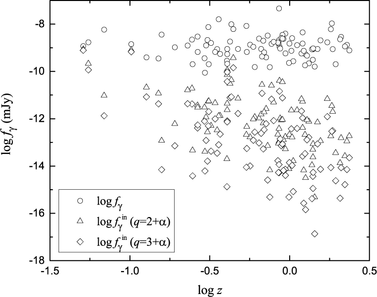
Fig. 1 Plot of γ-ray flux density versus redshift for the whole sample of 91 blazars. Circles stand for observed values, triangles stand for intrinsic values estimated in the case of  and rhombuses stand for intrinsic values estimated in the case of
  .
.
Download figure:
Standard imageBL Lacs: For the 32 BL Lacs, we have

with r = −0.10 and p = 59.96%;

with r = −0.45 and p = 1.03% for  ; and
; and

with r = −0.44 and p = 1.13% for  . The corresponding figure is shown in the upper panel of Figure 2
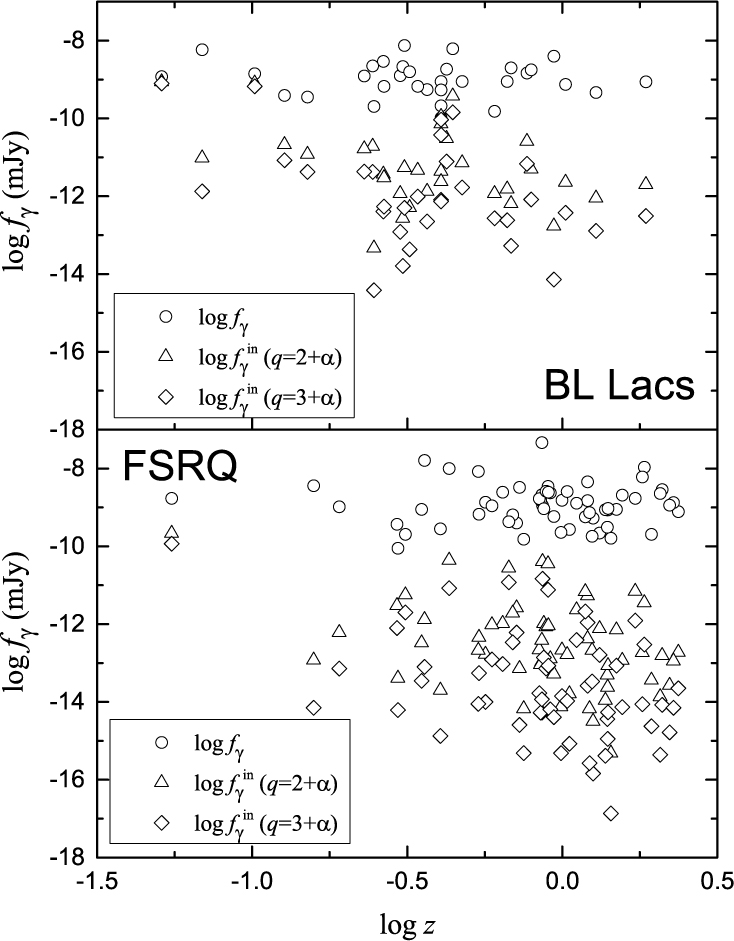
Fig. 2 Plot of γ-ray flux density versus redshift for 32 BL Lacs (upper panel) and 59 FSRQs (lower panel). Circles stand for observed values, triangles stand for intrinsic values estimated in the case of  , and rhombuses stand for intrinsic values estimated in the case of
  .
.
Download figure:
Standard imageFSRQs: For the 59 FSRQs, we have

with r = −0.01 and p = 94.20%;

with r = −0.37 and  for
for  ; and
; and

with r = −0.39 and  for
for  . The corresponding figure is shown in the lower panel of Figure 2.
ISP: For the 40 ISP blazars, we have

with r = −0.09 and p = 58.81%;

with r = −0.44 and  for
for  ; and
; and

with r = −0.45 and  for
for  . The corresponding figure is shown in the upper panel of Figure 3.

Fig. 3 Plot of γ-ray flux density versus redshift for 40 ISP blazars (upper panel) and 51 LSP blazars (lower panel). Circles stand for observed values, triangles stand for intrinsic values estimated in the case of  , and rhombuses stand for intrinsic values estimated in the case of
  .
.
Download figure:
Standard imageLSP: For the 51 LSP blazars, we have

with r = 0.06 and p = 68.03%;

with r = −0.54 and  for
for  ; and
; and

with r = −0.55 and  for
for . The corresponding figure is shown in the lower panel of Figure 3.
2.3. Short Variability Time Scale and Luminosity
Observations suggest that γ-ray loud blazars are variable on time scales of hours although there is no preferred scale for the variation time of any source (Fan et al. 2014a). For example, Fermi/LAT detected a variability time scale of ∼12 hours for PKS 1454 − 354 (Abdo et al. 2009), and a doubling time of roughly four hours for PKS 1502+105 (Abdo et al. 2010b). In the literature, available short variability time scales are collected, e.g., Bassani et al. (1983), Dondi & Ghisellini (1995), Fan et al. (1999b), Gupta et al. (2012) and Vovk & Neronov (2013).
For the sources with available short variability time scales, and X-ray and γ-ray emissions, we can estimate their γ-ray Doppler factors. Following our recent work (Fan et al. 2013a, 2014a), a Doppler factor can be estimated using
where  is the variability time scale in units of hours, α is the X-ray spectral index,
  is the flux density at 1 keV in units of
  ,
,  is the energy in units of GeV at which the γ-rays are detected, and
  is the luminosity distance in units of Mpc. The average energy
  can be calculated by
  , and the luminosity distance can be expressed in the form
from the  -CDM model (Capelo & Natarajan 2007) with
  ,
,  and
and  . We adopt
 throughout the paper. Then, we estimate the γ-ray Doppler factors (
 ) of 63 blzazrs and show them in Table 2.
Table 2. Short Variability Time Scales and γ-ray Doppler Factors for Fermi Blazars
| 3FGL name (1) | Other name (2) | z (3) | Class (4) |
 (5) (5) |
Band (6) | Ref. (7) |
 (8) (8) |
Ref. (9) |
 (10) (10) |
Ref.(11) |
 (12) (12) |
 (13) (13) |
 (14) (14) |
|---|---|---|---|---|---|---|---|---|---|---|---|---|---|
| J0141.4–0929 | 1Jy 0138–097 | 1.034 | B | 6.03 | γ | V13 | 0.70 | LAC | 1.15 | F14 | 20.65 | 2.12 | 4.45 |
| J0205.0+1510 | 4C +15.05 | 0.405 | Q | 5.78 | γ | V13 | 0.02 | BZC | 0.37 | E14 | 6.71 | 2.53 | 0.99 |
| J0210.7–5101 | PKS 0208–512 | 0.999 | Q | 5.61 | γ | V13 | 1.62 | LAC | 1.06 | B97 | 47.40 | 2.30 | 5.61 |
| J0222.6+4301 | 3C 66A | 0.444 | B | 5.10 | γ | V13 | 6.39 | LAC | 1.60 | F14 | 192.78 | 1.94 | 4.46 |
| J0238.6+1636 | PKS 0235+164 | 0.940 | B | 5.94 | γ | V13 | 1.24 | BZC | 1.59 | F14 | 103.05 | 2.17 | 4.41 |
| J0339.5–0146 | PKS 0336–01 | 0.852 | Q | 6.02 | γ | V13 | 0.75 | BZC | 0.62 | E14 | 33.58 | 2.42 | 3.67 |
| J0423.2–0119 | PKS 0420–01 | 0.915 | Q | 5.37 | γ | V13 | 3.87 | LAC | 0.86 | F14 | 55.92 | 2.30 | 6.84 |
| J0442.6–0017 | PKS 0440–00 | 0.844 | Q | 4.95 | γ | V13 | 4.06 | LAC | 0.59 | E14 | 34.94 | 2.50 | 8.05 |
| J0457.0–2324 | PKS 0454–234 | 1.003 | Q | 4.83 | γ | V13 | 0.60 | BZC | 0.48 | E14 | 180.35 | 2.21 | 7.31 |
| J0501.2–0157 | PKS 0458–02 | 2.286 | Q | 5.73 | γ | V13 | 0.92 | BZC | 0.60 | E14 | 23.24 | 2.41 | 12.30 |
| J0510.0+1802 | PKS 0507+17 | 0.416 | Q | 4.03 | γ | L15 | 0.38 | BZC | 0.50 | E14 | 13.34 | 2.41 | 4.34 |
| J0522.9–3628 | PKS 0521–36 | 0.055 | Q | 4.57 | γ | V13 | 22.50 | LAC | 0.92 | A09a | 47.34 | 2.44 | 2.27 |
| J0530.8+1330 | PKS 0528+134 | 2.070 | Q | 5.24 | γ | D95 | 3.75 | LAC | 0.58 | F14 | 36.86 | 2.51 | 17.83 |
| J0538.8–4405 | PKS 0537–441 | 0.894 | B | 6.04 | γ | V13 | 4.53 | LAC | 1.12 | F14 | 329.60 | 2.04 | 5.36 |
| J0540.0–2837 | 1Jy 0537–286 | 3.104 | Q | 6.21 | γ | V13 | 1.46 | LAC | 0.32 | F14 | 7.91 | 2.78 | 16.66 |
| J0721.9+7120 | 1H 0717+714 | 0.310 | B | 4.80 | γ | V13 | 4.91 | LAC | 1.77 | F14 | 219.99 | 2.04 | 3.62 |
| J0738.1+1741 | PKS 0735+17 | 0.424 | B | 6.05 | γ | V13 | 2.09 | LAC | 1.34 | F14 | 54.82 | 2.01 | 2.69 |
| J0739.4+0137 | PKS 0736+01 | 0.191 | Q | 4.86 | Opt | B83 | 6.36 | LAC | 0.76 | F14 | 27.34 | 2.48 | 2.94 |
| J0831.9+0430 | PKS 0829+046 | 0.230 | B | 6.06 | γ | V13 | 0.60 | BZC | 1.00 | L16 | 33.88 | 2.24 | 1.40 |
| J0841.4+7053 | RBS 0717 | 2.218 | Q | 4.41 | γ | V13 | 10.70 | LAC | 0.42 | F14 | 12.58 | 2.84 | 37.76 |
| J0854.8+2006 | PKS 0851+202 | 0.306 | B | 5.11 | γ | V13 | 1.79 | BZC | 1.50 | F14 | 59.03 | 2.18 | 2.81 |
| J0920.9+4442 | S4 0917+44 | 2.189 | Q | 5.08 | γ | V13 | 1.83 | LAC | 0.39 | F14 | 57.84 | 2.29 | 19.74 |
| J0957.6+5523 | 4C +55.17 | 0.901 | Q | 5.50 | γ | V13 | 0.77 | LAC | 0.84 | F14 | 104.50 | 2.00 | 5.10 |
| J0958.6+6534 | S4 0954+65 | 0.367 | B | 5.67 | γ | V13 | 1.12 | LAC | 0.24 | F14 | 13.81 | 2.38 | 2.26 |
| J1104.4+3812 | Mkn 421 | 0.031 | B | 3.84 | X | D95 | 678.00 | LAC | 1.82 | F14 | 302.58 | 1.77 | 4.13 |
| J1159.5+2914 | B2 1156+29 | 0.729 | Q | 5.59 | γ | V13 | 1.49 | LAC | 0.86 | F14 | 83.65 | 2.21 | 4.40 |
| J1217.8+3007 | 1ES 1215+303 | 0.130 | B | 4.18 | Opt | G12 | 86.40 | LAC | 1.47 | B00 | 60.51 | 1.97 | 4.66 |
| J1221.4+2814 | W Comae | 0.102 | B | 3.79 | Opt | F99b | 2.29 | LAC | 1.24 | F14 | 41.23 | 2.10 | 2.80 |
| J1224.9+2122 | PG 1222+216 | 0.432 | Q | 3.64 | γ | V13 | 3.82 | LAC | 1.19 | F14 | 255.37 | 2.29 | 6.68 |
| J1229.1+0202 | PKS 1226+02 | 0.158 | Q | 4.70 | γ | V13 | 111.00 | LAC | 1.11 | F14 | 94.24 | 2.66 | 4.21 |
| J1256.1–0547 | 3C 279 | 0.536 | Q | 5.48 | γ | V13 | 40.50 | LAC | 0.84 | F14 | 205.75 | 2.34 | 6.29 |
| J1310.6+3222 | B2 1308+32 | 0.997 | Q | 2.65 | Opt | B83 | 0.85 | LAC | 0.86 | B97a | 36.53 | 2.25 | 17.12 |
| J1408.8–0751 | PKS B1406–076 | 1.494 | Q | 4.76 | γ | F99a | 0.53 | BZC | 0.07 | F13 | 17.90 | 2.38 | 12.84 |
| J1439.2+3931 | PG 1437+398 | 0.344 | B | 6.25 | γ | V13 | 17.90 | LAC | 1.33 | F14 | 4.44 | 1.77 | 3.25 |
| J1457.4–3539 | PKS 1454–354 | 1.424 | Q | 4.64 | γ | A09b | 0.51 | BZC | 0.68 | E14 | 66.18 | 2.29 | 10.41 |
| J1504.4+1029 | PKS 1502+106 | 1.839 | Q | 4.16 | γ | A10 | 0.16 | BZC | 0.84 | F14 | 239.96 | 2.24 | 12.98 |
| J1512.8–0906 | PKS 1510–089 | 0.360 | Q | 3.84 | γ | V13 | 1.15 | BZC | 0.98 | F14 | 411.05 | 2.36 | 4.73 |
| J1517.6–2422 | AP Librae | 0.049 | B | 2.95 | Opt | B83 | 2.92 | LAC | 1.36 | F14 | 52.34 | 2.11 | 2.89 |
| J1535.0+3721 | RGB J1534+372 | 0.143 | B | 6.42 | γ | V13 | 0.37 | LAC | 1.84 | F14 | 4.10 | 2.11 | 1.07 |
| J1540.8+1449 | PKS 1538+149 | 0.605 | B | 3.44 | Opt | F96 | 1.82 | LAC | 0.66 | F14 | 3.70 | 2.34 | 9.88 |
| J1626.0–2951 | PKS 1622–297 | 0.815 | Q | 4.14 | γ | M97 | 2.28 | LAC | 0.45 | E14 | 25.02 | 2.45 | 10.66 |
| J1635.2+3809 | B3 1633+382 | 1.814 | Q | 4.81 | γ | V13 | 0.17 | BZC | 0.62 | F14 | 114.44 | 2.40 | 10.22 |
| J1642.9+3950 | 3C 345 | 0.593 | Q | 5.05 | Opt | D95 | 4.07 | LAC | 0.81 | F14 | 25.12 | 2.45 | 5.37 |
| J1653.9+3945 | Mkn 501 | 0.034 | B | 5.40 | Inf | B83 | 65.10 | LAC | 1.36 | F14 | 97.38 | 1.72 | 1.96 |
| J1728.3+5013 | I Zw 187 | 0.055 | B | 5.61 | X | B83 | 39.60 | LAC | 1.39 | F14 | 10.81 | 1.96 | 1.86 |
| J1733.0–1305 | PKS 1730–130 | 0.902 | Q | 4.90 | γ | V13 | 6.32 | LAC | 0.50 | F14 | 55.89 | 2.35 | 10.02 |
| J1740.3+5211 | S4 1739+52 | 1.379 | Q | 5.70 | γ | V13 | 1.25 | LAC | 1.08 | F14 | 16.66 | 2.45 | 6.85 |
| J1748.6+7005 | S4 1749+70 | 0.770 | B | 4.68 | γ | V13 | 1.55 | LAC | 1.44 | F14 | 41.38 | 2.06 | 6.14 |
| J1751.5+0939 | OT 081 | 0.322 | B | 5.47 | γ | V13 | 1.18 | BZC | 0.74 | L15 | 42.51 | 2.25 | 2.39 |
| J1800.5+7827 | S5 1803+78 | 0.684 | B | 4.95 | γ | V13 | 1.71 | LAC | 0.45 | F14 | 50.65 | 2.22 | 5.97 |
| J1806.7+6949 | 3C 371 | 0.051 | B | 4.92 | Opt | B83 | 4.79 | LAC | 0.75 | F14 | 33.48 | 2.23 | 1.49 |
| J1813.6+3143 | B2 1811+31 | 0.117 | B | 6.26 | γ | V13 | 1.44 | LAC | 2.60 | L15 | 15.44 | 2.12 | 1.27 |
| J1824.2+5649 | S4 1823+56 | 0.664 | B | 6.60 | γ | V13 | 2.52 | LAC | 0.96 | F14 | 20.11 | 2.46 | 2.86 |
| J1833.6–2103 | PKS 1830–210 | 2.507 | Q | 4.44 | γ | V13 | 3.25 | LAC | 0.13 | F14 | 15.44 | 2.12 | 43.49 |
| J2009.3–4849 | 1Jy 2005–489 | 0.071 | B | 6.48 | γ | V13 | 80.80 | LAC | 1.32 | F14 | 35.54 | 1.77 | 1.78 |
| J2134.1–0152 | PKS 2131–021 | 1.285 | B | 5.88 | γ | V13 | 0.67 | LAC | 1.05 | F14 | 11.18 | 2.21 | 5.66 |
| J2143.5+1744 | S3 2141+17 | 0.211 | Q | 5.45 | γ | V13 | 1.76 | LAC | 1.44 | F14 | 44.18 | 2.52 | 1.92 |
| J2158.8–3013 | PKS 2155–304 | 0.117 | B | 6.69 | γ | V13 | 572.00 | LAC | 1.62 | F14 | 216.84 | 1.83 | 2.64 |
| J2202.7+4217 | B3 2200+420 | 0.069 | B | 4.96 | γ | V13 | 7.42 | LAC | 0.83 | F14 | 164.77 | 2.25 | 1.81 |
| J2225.8–0454 | 3C 446 | 1.404 | Q | 3.48 | Opt | B83 | 2.12 | LAC | 0.59 | F14 | 19.43 | 2.36 | 22.99 |
| J2232.5+1143 | PKS 2230+11 | 1.037 | Q | 4.63 | Opt | B83 | 3.06 | LAC | 0.51 | F14 | 50.19 | 2.52 | 11.05 |
| J2250.1+3825 | B3 2247+381 | 0.119 | B | 6.15 | γ | V13 | 7.93 | LAC | 1.51 | F14 | 11.02 | 1.91 | 1.69 |
| J2254.0+1608 | PKS 2251+15 | 0.859 | Q | 2.94 | γ | V13 | 19.00 | LAC | 0.62 | F14 | 1060.92 | 2.35 | 26.71 |
Note: Column (1) gives the Fermi name; Col. (2) other name; Col. (3) redshift; Col. (4) classification, "B" stands for BL Lacs and "Q" stands for FSRQs; Col. (5) short variability time scale ( ) in units of s; Col. (6) band at which
  is detected; Col. (7) references for Cols. (3), (5) and (6); Cols. (8) and (9) X-ray flux in units of
 at 0.1–2.4 keV and its reference respectively; Cols. (10) and (11) X-ray spectral index and its reference respectively; Cols. (12) and (13) γ-ray integral photon flux at 1–100 GeV in units of
 and photon spectrum index (
 ) from 3LAC respectively; Col. (14) γ-ray Doppler factor (
 ). Here, LAC: Ackermann et al. 2015; BZC: Massaro et al. (2015); A09a: Ajello et al. (2009); A09b: Abdo et al. (2009); A10: Abdo et al. (2010b); B83: Bassani et al. (1983); B97: Brinkmann et al. (1997); B00: Brinkmann et al. (2000); D95: Dondi & Ghisellini (1995); E14: Evans et al. (2014); F96: Fan & Lin (1996); F99a: Fan et al. (1999b); F99b: Fan et al. (1999a); F09: Fan et al. (2009); F13: Fan et al. (2013a); F14: Fan et al. (2014a); G12: Gupta et al. (2012); H09: Hovatta et al. (2009); LB15: Liao & Bai (2015); LF16: Lin & Fan (2016); LV99: Lähteenmäki & Valtaoja (1999); M97: Mattox et al. (1997); S10: Savolainen et al. (2010); V13: Vovk & Neronov (2013). If a source has short variability time scales in different references, the value in the latest one is considered.
To compare γ-ray Doppler factors estimated in this work with radio Doppler factors, we show the plot of γ-ray Doppler factors versus radio Doppler factors in Figure 4. We find that the γ-ray Doppler factors that we estimated are on average lower than the radio Doppler factors. The reason may be from the fact that the derived value in this work is a lower value as discussed in Fan et al. (2014a).

Fig. 4 Plot of γ-ray Doppler factors estimated in this work versus radio Doppler factors from corresponding references.
Download figure:
Standard imageThe luminosity can be calculated using  , where
  is the integral flux calculated by Equation (2) and
  stands for a K-correction into the source rest frame (Fan et al. 2013b; Kapanadze 2013). In a beaming model, the observed photon energy is also beamed,
  , where
  is the intrinsic energy. Because
  , we have
  for the case of
  ,
,  for the case of
  , and
, and  . Here
  and
and  are the intrinsic luminosity and the intrinsic variability time scale respectively.
For calculating  and
and  , we use radio Doppler factors in Table 1, but if there is no available radio Doppler factor, we substitute γ-ray Doppler factors in Table 2 instead. When the Doppler boosting effect is considered, the plot of short variability time scale versus γ-ray luminosity is shown in Figure 5, where both observed properties and intrinsic properties are shown. Then we find that nine blazars violate the E-S or A-N Relation in
  versus
  . However, the whole sample follows the E-S and A-N Relations in
  versus
  , see Figure 5. When the subclasses of blazars are considered, nine FSRQs violate the E-S Relation and three FSRQs violate the A-N Relation in observed data, but all blazars follow those relations in intrinsic data, see Figure 6.
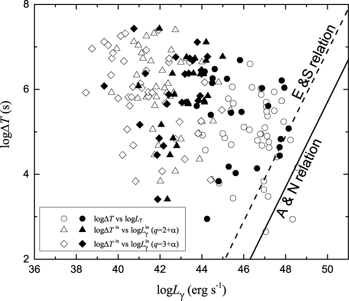
Fig. 5 Plot of short variability time scale versus γ-ray luminosity. Circles stand for observed values, triangles stand for intrinsic values estimated in the case of  and rhombuses stand for intrinsic values estimated in the case of
  . Filled symbols stand for sources whose intrinsic values are estimated by the γ-ray Doppler factors, while open symbols stand for those by radio Doppler factors.
Download figure:
Standard image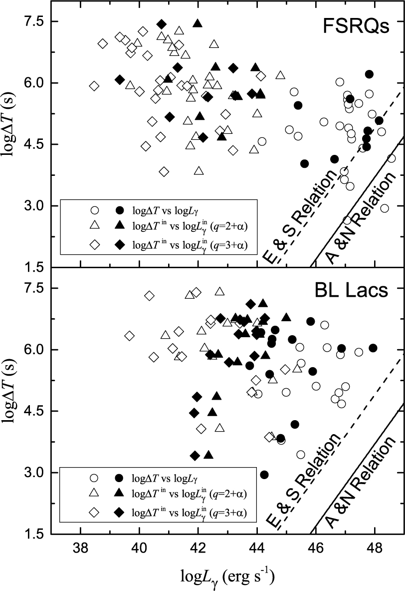
Fig. 6 Plot of short variability time scale versus γ-ray luminosity for 31 FSRQs (upper panel) and 26 BL Lacs (lower panel). Circles stand for observed values, triangles stand for intrinsic values estimated in the case of  , and rhombuses stand for intrinsic values estimated in the case of
  . Filled symbols stand for sources whose intrinsic values are estimated by γ-ray Doppler factors, while open symbols stand for those by radio Doppler factors.
Download figure:
Standard image2.4. γ-ray Emissions and Synchrotron Peaked Frequency
For the whole sample of 91 blazars, linear regression analysis is applied to the correlations between γ-ray flux density ( ) and synchrotron peak frequency (
 ). The synchrotron peak frequencies are corrected to the rest frame by
  before analysis.
For  –
– correlation, we have

with r = 0.07 and p = 51.51%,

with r = 0.65 and  for
for  , and
, and

with r = 0.68 and  for
for  ; here
  is an intrinsic peak frequency. The corresponding figure is shown in Figure 7.

Fig. 7 Plot of γ-ray flux density versus synchrotron peak frequency for the whole sample of 91 blazars. Circles stand for observed values, triangles stand for intrinsic values estimated in the case of  , and rhombuses stand for intrinsic values estimated in the case of
  .
.
Download figure:
Standard imageAs results show in Section 2.2 and in Lin & Fan (2016), γ-ray flux density is strongly correlated with redshift, therefore the correlations between γ-ray emissions and peak frequency may be caused by a redshift effect. In our recent works (Fan et al. 2013b; Fan et al. 2015a; Lin & Fan 2016), we have removed the redshift effect from the luminosity-luminosity correlation by using the partial correlation introduced by Padovani (1992). If variables i and j are correlated with a third one k, then the correlation between i and j can remove the k effect, as follows:
where  ,
,  and
and  are the correlation coefficients between any two variables of i, j and k respectively. When the method is applied to the
correlation, the correlation coefficients excluding the redshift effect for the whole sample are as follows:  = 0.56 with
  for
for  and
and  = 0.59 with
  for
for  .
.
3. Discussion and Conclusions
In this work, we collect 91 blazars with available radio Doppler factors, and calculate their intrinsic γ-ray flux density ( ) at 2 GeV and intrinsic synchrotron peak frequency (
 ). Then the correlations between
  and redshift, and between
  and
and  are investigated. We also study the intrinsic relation between short variability time scale (
 ) and γ-ray luminosity (
 ) for 63 blazars by comparing to the E-S and A-N Relations.
In our recent work, we compared the γ-ray Doppler factors ( ) with the radio Doppler factors (
 ), and found they are associated with each other, see Fan et al. (2014a). So, we can investigate the beaming effect in the γ-ray band by using the radio Doppler factors. We also found that the radio Doppler factor correlates well with γ-ray luminosity for the Fermi detected sources, see Fan et al. (2009). In this work, we find that values of
  of FSRQs are smaller than those of BL Lacs with a probability for the two groups to come from the same distribution (Kolmogorov-Smirnov (K-S) test) being
  for
for  and
and  . The averaged values of
  are
are
for FSRQs; and
for BL Lacs. a t-test indicates that the averaged difference of  between BL Lacs and FSRQs is
with a significance level of  for
for  , and
, and  with
with  for
for  , while the averaged difference of the observed flux density (
 ) is
) is  with p = 64.23%.
3.1. γ-ray Flux Density and Redshift
We analyze the whole sample of 91 Fermi blazars, and find that  is weakly correlated with redshift (r = −0.01, and slope is −0.01 ± 0.15). The result is different from our expectation:
  , if blazars belong to a group. But when we consider the strong beaming effect of γ-ray emissions for Fermi blazars, we find that
  is strongly correlated with redshift as follows:
  with r = −0.54 and
  for
for  , and
, and  with
with  and
and  for
for  . In our recent work (Xiao et al. 2015), we found that
  and redshift have a strong correlation (
 ) with the slopes being −2.05 ± 0.32 (
 ) and −2.55 ± 0.34 (
 ) respectively. Results in the present work suggest that
  and redshift follow the theoretical relation, which is consistent with our previous work (Xiao et al. 2015).
For subclasses of blazars, some similar correlation results are found, but their slopes are slightly different. The slopes of correlations between  and redshift are −1.30 ± 0.47 (BL Lacs), −1.34 ± 0.45 (FSRQs), −1.33 ± 0.44 (ISP) and −1.95 ± 0.44 (LSP) for the case of
  ; and those are −1.65 ± 0.61 (BL Lacs), −1.73 ± 0.55 (FSRQs), −1.67 ± 0.54 (ISP) and −2.51 ± 0.55 (LSP) for
  . In our results, slopes of BL Lacs are very close to those of FSRQs, and they favor the jet case of
  . However, for the whole sample, the results of slopes indicate that two jet cases exist in blazars, since slopes are −1.82 ± 0.30 for
  , − 2.32 ± 0.37 for
  , and ∼ −2.0 for the theoretical relation. For the SED classification, results of slopes suggest that ISP blazars favor the jet case of
  , while LSP blazars favor the jet case of
  . Those results indicate stationary jets (
 ) are perhaps dominant in LSP blazars. A possible explanation of those results is the differences in synchrotron peaked frequency caused by the physical differences in blazars, such as the different forms of relativistic jets. In Xiao et al. (2015), we suggested that the continuous case (
 ) of a jet is perhaps real for Fermi blazars, however, we did not discuss the subclasses in that work. In the present work, we cannot discuss this further since there is no Doppler factor for HSP blazars.
3.2. Short Variability Time Scale and Luminosity
For the whole sample of 63 blazars, our results show that nine blazars violate the E-S or A-N Relation in  versus
  , but the whole sample follows the E-S and A-N Relations in
  versus
  , see Figures 5 and 6.
In our recent work (Xiao et al. 2015), some similar results are found for a sample of 28 blazars. Different subclasses of blazars have different properties, for instance FSRQs have strong emission lines, so that their redshifts can be determined more easily and accurately than those of BL Lacs, and FSRQs statistically have higher redshift and lower synchrotron peaked frequency than BL Lacs. Therefore, for further analysis, the subclasses of blazars are considered. We find that nine FSRQs violate the E-S Relation and three FSRQs violate the A-N Relation in  versus
  , but all blazars follow those relations in their intrinsic properties. In addition, the averaged values of radio Doppler factors are
  for 32 BL Lacs and
  for 59 FSRQs. From a K-S test, the probability that the distributions of
  for BL Lacs and FSRQs are drawn from the same parent distribution is
  . Thus, the Doppler factors of FSRQs are larger than those of BL Lacs, which is consistent with our previous result (Fan et al. 2004). From the above analysis, we find that the beaming effect is an important reason that causes blazars to violate the E-S and A-N Relations, and FSRQs have a stronger beaming effect than BL Lacs.
3.3. γ-ray Emissions and Synchrotron Peaked Frequency
There is no correlation between  and
and  with r = 0.07 and p = 51.51%. However, strong positive correlations are found between
  and
and  for the whole sample. Those correlation coefficients and chance probabilities are r = 0.65 and
  for the case of
  , and r = 0.68 and
  for
for  respectively. When the redshift effect is removed, strong positive correlations still exist between them. In Lister et al. (2011), strong anti-correlations are found between observed radio flux density at 5 GHz and synchrotron peak frequency for BL Lacs and FSRQs. From results in Lister et al. (2011) and this work, the anti-correlations (or no correlation) between observed flux densities and synchrotron peak frequency are significantly different from the positive correlations in intrinsic properties. Thus, the beaming effect cannot be ignored when we investigate the physical mechanism of blazars.
The blazar sequence, which is defined by the anti-correlation between peak luminosity and peak frequency, can be explained by the cooling effect (Fossati et al. 1998; Ghisellini et al. 1998; Wu et al. 2007; Nieppola et al. 2008). However, that theoretical explanation of the blazar sequence does not consider the beaming effect. Therefore, the intrinsic correlation between peak luminosity and peak frequency is needed to investigate the blazar sequence. Wu et al. (2007) estimated Doppler factors ( ) for a sample of 170 BL Lacs and found significant anti-correlations between
  and
and  , and between the total 408 MHz luminosity (
 ) and
) and  . However, the scatter of
  versus
  is very large, which is in contrast with the much tighter relation of blazar sequence. Some similar results are found between radio power and
  in Nieppola et al. (2006). Recently, some high-luminosity high-
 and low-luminosity low-
 sources have been detected. Those results indicate that the blazar sequence is likely to be eliminated (Wu et al. 2007).
Nieppola et al. (2008), who collected a sample of 89 AGNs with available Doppler factors, found strong anti-correlation between  and
and  , and proposed that the lower peak frequency blazars are more boosted. In Nieppola et al. (2008), a positive Spearman rank correlation between intrinsic synchrotron peak luminosity (
 ) and
) and  was also found with r = 0.366 and
  for blazars, especially for BL Lacs (r = 0.642 and
  ). They concluded that the anti-correlation between
  and
and  which is used to determine the blazar sequence is not present, suggesting that the blazar sequence is an artifact of variable Doppler boosting across the peak frequency range. However, scatter in the correlation between
  and
and  is about five orders of magnitude for their sample. In addition, Wu et al. (2009) found a significant positive
  –
– correlation with a Spearman correlation coefficient of r = 0.59 at the > 99.99% confidence level. In this work, we find a positive correlation between
  and
and  after correcting the redshift effect. Thus, our results and previous research indicate that there is a positive correlation between intrinsic emissions and intrinsic synchrotron peak frequency.
Interestingly, we find a strong positive correlation between  and
and  :
:  with r = 0.91 and
  . The strong positive
  –
– correlation indicates that there is almost no difference in the order of blazars along the peak frequency between before and after considering the beaming effect. Thus, intrinsic properties of the blazar order would not be eliminated, although the relation between luminosity and peak frequency is changed significantly. The observed blazar order is strongly associated with the intrinsic one. Therefore, a new theoretical explanation is needed for the intrinsic blazar order. In addition, we noticed that the intrinsic blazar order could change what we know about blazars, such as differences in black hole mass between BL Lacs and FSRQs.
The positive correlation between γ-ray emissions and peak frequency indicates that the synchrotron emissions are highly correlated with γ-ray emissions. From the synchrotron self-Compton (SSC) process, γ-ray emissions are produced by the inverse Compton scattering process from synchrotron emissions, so that they should be associated with each other. In addition, we suppose that  and
and  relations can be used to estimate the Doppler boosting factors. However, a larger sample is needed to find more accurate correlations.
3.4. Conclusions
In this work, we collect 91 Fermi blazars with available Doppler factors, and investigate the correlations between intrinsic flux density and redshift for the whole sample, BL Lacs, FSRQs, ISP and LSP separately. Then, we estimate γ-ray Doppler factors of 63 blazars, and study the relationship between γ-ray luminosity and short variability time scale for those blazars. The observed and intrinsic correlations between the γ-ray flux density and synchrotron peak frequency are also investigated for the whole blazar sample. Our main conclusions are as follows:
- (1)The correlation between
 and redshift follows the theoretical relation: . When the subclasses are considered, we find that the stationary jets are perhaps dominant in LSP blazars.
 - (2)Nine FSRQs violate the E-S or A-N Relation in versus , while the whole blazar sample obeys the E-S and A-N Relations in versus . Thus, FSRQs have a stronger beaming effect than BL Lacs.
- (3)Strong positive correlation between and is found, which suggests that synchrotron emissions are highly correlated with γ-ray emissions.


Acknowledgments
This work is supported by the National Natural Science Foundation of China (Grant Nos. U1531245, U1431112, 11203007, 11403006, 10633010, 11173009 and 11403006), and the Innovation Foundation of Guangzhou University (IFGZ), Guangdong Innovation Team (2014KCXTD014), Guangdong Province Universities and Colleges Pearl River Scholar Funded Scheme (GDUPS) (2009), Yangcheng Scholar Funded Scheme (10A027S), and support for Astrophysics Key Subjects of Guangdong Province and Guangzhou City.