
Abstract
Based on the hybrid solutions to (2+1)-dimensional Kadomtsev–Petviashvili (KP) equation, the motion trajectory of the solutions to KP equation is further studied. We obtain trajectory equation of a single lump before and after collision with line, lump, and breather waves by approximating solutions of KP equation along some parallel orbits at infinity. We derive the mathematical expression of the phase change before and after the collision of a lump wave. At the same time, we give some collision plots to reveal the obvious phase change. Our method proposed to find the trajectory equation of a lump wave can be applied to other (2+1)-dimensional integrable equations. The results expand the understanding of lump, breather, and hybrid solutions in soliton theory.
Export citation and abstract BibTeX RIS
1. Introduction
For the research on nonlinear complex phenomena, nonlinear partial differential equations play an essential role. And nonlinear partial differential equations have gained many applications, such as nonlinear optics, fluid mechanics, and so forth.[1–3] The (2 + 1)-dimensional Kadomtsev–Petviashvili equation can give perfect descriptions of the nonlinear and long waves with small amplitudes. In soliton theory, the problems of hybrid solutions and lumps have attracted more and more attention from experts in recent years.[4,5]
In this paper, we consider the (2 + 1)-dimensional Kadomtsev–Petviashvili equation[6] as follows:

where u = u(x, y, t) denotes a scalar function of the space variables x, y, and time variable t, α is a constant depending on the dispersive property of the system. α > 0 corresponds to negative dispersion and vice versa.
Under the variable transformation:

where f(x, y, t) is a complex function. Inserting Eq. (2) into Eq. (1) yields

The operator D is the Hirota's bilinear differential operator defined by
In the work of Satsuma,[7] the N soliton solution can be ascertained by direct methods
with
where ∑μ = 0,1 denotes the summation which takes over all possible combinations of μj, μs = 0,1, s, j = 1,2,..., N.
Lump and hybrid solutions to Eq. (1) can be generated from soliton solutions by taking a long wave limit.[8,9] In order to obtain n-th order lump solutions, we take a long wave limit with the provision in Eq. (5):
General higher-order lump solutions to Eq. (1) can be expressed in the following forms:

where
with
More specifically, such solutions can be studied by searching for positive quadratic functions.[10–17]
In order to obtain a hybrid of m lumps and n breathers,[18] we can take a long wave limit with the following provision in Eq. (5)
Similarly, in order to obtain a hybrid of m lumps and n line waves,[19] we can take a long wave limit with the following procvision in Eq. (5):
In other words, on the basis of N-soliton solutions, using the long wave limit method, we can obtain a variety of semi-rational solutions, namely a hybrid of lumps and line waves, a hybrid of lumps and breathers, a hybrid of lumps, breathers, and line waves. In Ref. [4], the interactions of a lump with a line wave for (2+1)-dimensional Sawada–Kotera equation have been considered. The authors have given the asymptotic behaviors and phase shifts of a lump and a solitary wave. In Ref. [20], the authors discussed interactions of a lump and a breather wave for the positive KP equation and gave the phase shifts clearly. Further, we obtained more general trajectory equations of a single lump before and after collision with line, lump, and breather waves. In this paper, we find a way to approximate hybrid solutions at infinity along some parallel orbits and obtain the trajectory of a single lump in the hybrid solutions.
The arrangement of this paper is organized as follows: In Section 2, the trajectory of a lump is introduced. In Section 3, we mainly investigate a single lump in the hybrid solutions consisting of a lump and line waves. In Section 4, we describe how each lump moves among multiple lumps to Eq. (1). In Section 5, we mainly investigate the trajectory of a single lump in a hybrid of a lump and breather waves.
2. The trajectory of a lump
According to Eq. (2), Eq. (8), Eq. (10), and Eq. (11), the first-order lump wave solutions has the following form:

Here the constraint relations between parameters K1, K2, P1, P2 are given by Eq. (8) and θs, ajs are given by Eq. (11). We can obtain the nonsingular first-order lump wave solutions to Eq. (1) when α < 0 and the figures are shown in Fig. 1. By solving the equations ux = 0, uy = 0 and combining the positive and negative of uxx, uxxuyy − uxy2, we can obtain the peak of the first-order lump solutions to Eq. (1)
The motion trajectory and moving speed of the first-order lump solutions are
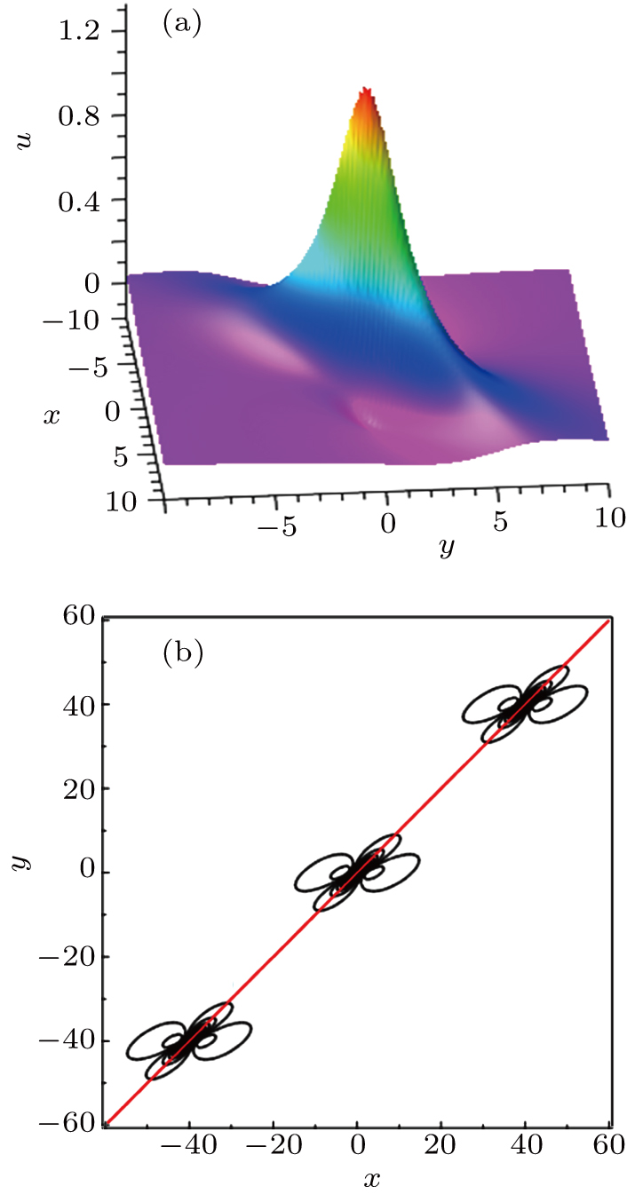
Fig. 1. The first-order lump solution to Eq. (1) with parameters α = −1,  , P1 = P2 = 2. (a) The first-order lump solution at t = 0; (b) The trajectory of the lump y = x.
Download figure:
Standard image3. The trajectory of a single lump in a hybrid of a lump and line waves
In this section, we mainly investigate the trajectory of a single lump in the a hybrid of a lump and line waves.
3.1. The trajectory of a single lump in a hybrid of a lump and a line wave
Before giving a general expression of a single lump in hybrid solutions to Eq. (1), it is necessary to give a concrete example to illustrate. According to the constraints of Eq. (13), we may assign the parameters: α = −1, K1 = −1 + i, K2 = −1 − i, P1 = 2, P2 = 2, k3 = 1, p3 = 2, and then we can get the following expression:
The corresponding hybrid solutions u defined by Eq. (2) with Eq. (17) are derived.
It can be clearly seen from Fig. 2 that after the collision of lump wave and line wave, the phase of lump wave changes significantly.
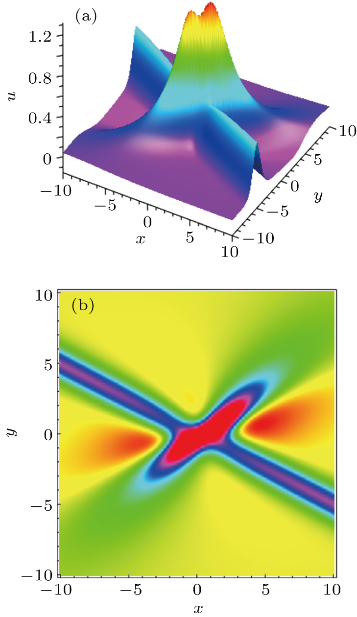
Fig. 2. A hybrid solutions consisting of a lump and a line wave to Eq. (1) at t = 0: (a) Three-dimensional plot; (b) Density plot.
Download figure:
Standard imageIn order to study the specific change value of the phase of the lump in the hybrid solutions. Combined with the law of motion of a single lump Eq. (15), the following constraints are imposed on Eq. (17):

where c1, c2 are real constants.
Then equation (17) becomes the following form:

Because c1, c2 are constants, when t ↦ − ∞, equation (19) can be approximated as the following equation:

Combined with the characteristics of equation (2), after Eq. (19) is divided by e9t + c1 + 2c2, it still corresponds to the solution of Eq. (1). So when t ↦ ∞, we can make the following approximation:

Again in combination with Eq. (18), equations (20) and (21) can be transformed into the following forms:
where f−inf corresponds to the state of the lump before the collision, and finf corresponds to the state after the collision of the lump. Referring to Eq. (14)–Eq. (16), we can separately find the motion trajectory of the peak before and after the collision
That is to say, after the collision, the moving speed of the peak have not changed. Just after the collision, the phase has changed. The peak moves along the yinf = −132/157 + xinf trajectory.
In order to give the trajectory equation of a lump wave before and after collision, it is necessary to define the following two functions:
If the hybrid solutions consisting of a lump and a line wave to Eq. (1) has the following form and λ3 ≠ 0:
with
Before and after the collision of a lump and a line wave, the trajectory equations of the peak are
with
The change in the phase of the lump wave before and after the collision is Δb3,
Here, sign(x) is a symbolic function and k3, p3, φ3 are real parameters. In Theorem 1, the relationships between parameters are constrained by Eq. (13).
Proofequation (26) is constrained as follows:
and then it converted to the following equation:
with
Similar to the method of Eq. (19)–Eq. (23), we can obtain the approximate expressions of Eq. (32) which tends to positive infinity and negative infinity at t. Let us first discuss the case of λ3 > 0,
The variables of Eq. (34) are replaced as follows:
Equation (34) is transformed into the following equation:
where f−inf corresponds to the state of the lump before the collision, and finf corresponds to the state after the collision of the lump. Referring to Eq. (14)–Eq. (16), we can separately find the motion trajectory of the peak before and after the collision
Equation (37) is consistent with Eq. (28), so equation (28) is proven. By converting Eq. (37) into an ordinary equation without parameter t, we can get the change value Δ b3 of phase of the lump wave before and after collision. The proof process for the case where λ3 < 0 is roughly the same as the above proof process, and we will not go into too much detail here.
3.2. The trajectory of a single lump in a hybrid of a lump and two line waves
If the hybrid solutions consisting of a lump and two line waves to Eq. (1) has the following form and λ3,λ4 ≠ 0:
with
and
Before and after the collision of a lump wave and two line waves, the trajectory equations of peak are respectively
The change in the phase of the lump wave before and after the collision is Δb,
with
Here, Ajs, ηs, θs, ws, hinf, h−inf, σs, γs are given by Eqs. (6), (7), (11), (24), and (29). k3, k4, p3, p4, ϕ3, ϕ4 are real parameters. In addition, the constraint relationships between the parameters are given by Eq. (13).
ProofEquation (39) becomes the following equation under the constraints of Eq. (31):
with

In the following, only the cases of λ3 > 0, λ4 > 0 and λ3 > 0, λ4 < 0 are discussed, other cases are similar to the two cases.
When λ3 > 0, λ4 > 0, since both βs and ηs are constants, similar to Eq. (34), equation (44) can be approximated to the following equation when time t approaches negative infinity and positive infinity:
Referring to Eqs. (34)–(36), we can separately find the motion trajectory of the peak before and after the collision
When λ3 > 0, λ4 > 0, equation (47) is the same as Eq. (41). By converting Eq. (47) into a normal equation that does not contain the parameter t, we are able to obtain the change in phase before and after the collision. The amount of phase change corresponds to Eq. (42).
When λ3 > 0, λ4 < 0, similar to Eq. (34), equation (44) can be approximated to the following equation when time t approaches negative infinity and positive infinity:
Referring to Eqs. (34)–(36), we can separately find the motion trajectory of the peak before and after the collision
We know from Eq. (49) that equation (41) is correct. According to Eq. (49), we can get the motion trajectory of the peak before and after the collision
According to Eq. (50), the amount of phase change before and after the collision is exactly Δb in Eq. (42).
In order to explain the role of Theorem 2 and to better explain the motion trajectory of the peak before and after the collision, the parameters in Eq. (36) can be assigned as follows: K1 = −1 + i, K2 = −1 – i, P1 = 2, P2 = 2, α = −1, k3 = 1, p3 = 2, ϕ3 = 0, k4 = 1, p4 = 7, ϕ4 = 0. From Fig. 3, we can observe that the phase of the lump wave changes significantly after the lump wave collides with the two line waves.

Fig. 3. A hybrid solutions consisting of a lump and two line waves to Eq. (1) at t = 0: (a) three-dimensional plot; (b) density plot.
Download figure:
Standard imageCombined with Theorem 2, we can get the parametric equations of the peak motion before and after the collision
That is to say, after the collision, the peak moves along the trajectory of yinf = xinf − 183282/181021, and the moving speed of the peak does not change, and is still  .
.
In addition, comparing Theorem 1 and Theorem 2, we will find that the interaction between a lump wave and two line waves can be understood as the superposition of the interaction between a lump wave and each line wave. Further, there is an inference as follows.
Inference 1If λ3, λ4,...,λ2 + m ≠ 0, then before and after the collision of a lump with m line waves, the motion trajectories of the peaks are
The change in the phase of the lump wave is
Here, h−inf, hinf, λs, γs, σs, Δbs are given by Eqs. (24), (29), (38), and (43). k3, k4,..., k2 + m, p3, p4,..., p2+m, and ϕ3, ϕ4,..., ϕ2+m are real parameters. In addition, the constraint relationships between the parameters are given by Eq. (13).
4. The trajectory of a single lump in the higher lump solutions
After a lump wave collides with a lump wave, the motion state of the lump wave has the following theorem: Theorem 3
If the second-order lump solutions to Eq. (1) has the following form and χ3, χ4 ≠ 0
with
then, before and after the collision of a lump with a lump wave, the trajectory equation of the peak does not change. The trajectory equation of the peak is
Here, ajs and θs are given by Eq. (11), and the constraint relationships between the parameters are given by Eq. (8).
The proof of Theorem 3 is roughly similar to the proof of Theorem 1, so it is not proved here. According to Theorem 3, we can get the motion trajectory before and after the collision of a lump wave and a lump wave. In order to better explain the role of Theorem 3 and the state before and after the collision of a lump wave and a lump wave, the parameters are assigned as follows: α = −1, K1 = −1 + i, K2 = −1 − i, P1 = 2, P2 = 2, K3 = 1 − i, K4 = 1 + i, P3 = − 2 i, P4 = 2i.
It can be seen from Fig. 4 that the trajectories of the peaks has not changed before and after the collision. The motion trajectories of the two peaks are x = 2t, y = 2t, and x = 2t, y = −2t.
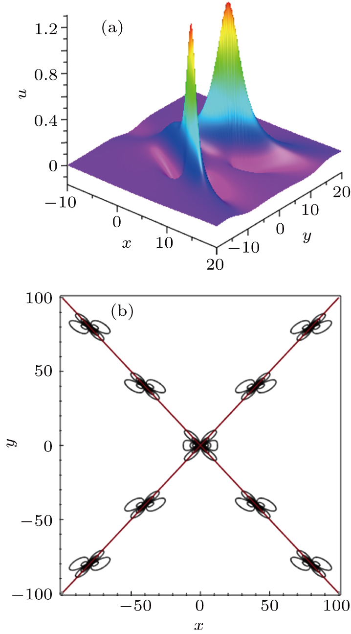
Fig. 4. The second-order lump solution to Eq. (1): (a) three-dimensional plot at t = 0; (b) schematic diagram of the movement path.
Download figure:
Standard imageFurther generalization, in the higher-order lump solutions to Eq. (1), the motion equation of the peak of a single lump wave is as shown in Eq. (56).
5. The trajectory of a single lump in a hybrid of a lump and breathers
Firstly, from the case where a lump wave collides with a breather wave, there is the following theorem.
Theorem 4If the hybrid solution consisting of a lump and a breathers to Eq. (1) has the following form and Re(λ3), Re(λ4) ≠ 0:

with
Before and after the collision of a lump wave and a breather wave, the trajectory equations of wave peak are respectively
The change in the phase of the lump wave before and after the collision is Δb,
Here, Ajs, ηs, θs, ws, γs, σs, λs, Δbs are given by Eqs. (6), (7), (11), (29), (38), and (43). k3, k4, p3, p4, ϕ3, ϕ4 are complex parameters. In addition, the constraint relationships between the parameters are given by Eq. (12).
Comparing Theorem 2 with Theorem 4, except for the preconditions and the constraints between the parameters are slightly different, but Theorem 2 is consistent with Theorem 4 from the formal point of view. This is because hybrid solutions consisting of a lump and a breather are obtained by conjugating certain parameters of hybrid solutions consisting of a lump and two line waves. The proof of Theorem 4 is roughly similar to the proof process of Theorem 2, so we will not go into too much detail here.
In order to better explain the role of Theorem 4 and to more clearly describe the collision between a lump wave and a breather wave, we assign the parameters as follows: K1 = −1 + i, K2 = −1 − i, P1 = 2, P2 = 2, k3 = 1/3 − i, k4 = 1/3 + i, p3 = 1, p4 = 1, ϕ3 = 0, ϕ4 = 0, α = −1.
From Fig. 5, we can get qualitative conclusions. After the lump wave collides with the breather wave, the trajectory of the lump wave changes. Combined with Theorem 4, we can get the motion trajectory of the peak before and after the collision between the lump wave and the breather wave: y−inf = x−inf, yinf = xinf − 292977456/146200249.

Fig. 5. Hybrid solutions consisting of a lump and a breather wave for Eq. (1). (a) Three-dimensional plot at t = 2; (b) density plot at t = −0.5.
Download figure:
Standard imageFurther generalizing Theorem 4, we get the following conclusion: Inference 2
If Re(λ3), Re(λ4),...,Re(λ2+2m) ≠ 0, then after a lump wave collides with m breather waves, the trajectories of peak are respectively
The change in the phase of the lump wave before and after the collision is Δb,
Here, Ajs, ηs, θs, ws, γs, σs, λs, Δbs are given by Eqs. (6), (7), (11), (29), (38), and (43). k3, k4,...,k2m + 2, p3, p4,...,p2m + 2, ϕ3, ϕ4, ϕ2m + 2 are complex parameters. In addition, the constraint relationships between the parameters are given by Eq. (12).
In addition, in the hybrid solutions consisting of lump waves, line waves and breather waves, the trajectory of a single lump can be obtained by using the Theorems 1, 2, 3, 4 in combination, and we will not make too much description.
6. Conclusion
In this paper, by approximating the solutions to the (2+1)-dimensional Kadomtsev–Petviashvili equation at infinity along some specific trajectories, we obtain the trajectory equation of a lump before and after collision with line, lump, and breather waves. Theorem 1, Theorem 2, and Inference 1 give the trajectory equation of a lump wave before and after the collision of a lump wave and line waves. Theorem 2 describes the collision of a lump and a lump wave. Theorem 4 and Inference 2 give the trajectory equation of a lump wave before and after the collision of a lump wave and breathers waves. Through the joint use of Theorems 1, 2, 3, 4, and Inferences 1, 2, we can get the trajectory equation of a lump wave in the hybrid solutions consisting of lump, breather, and line waves. Based on the trajectory equation of a lump wave before and after collision, we further obtain the general expressions of phase change, as shown in Eqs. (53) and (62). In addition, the method proposed here to find the trajectory equation of a lump wave can be extended to other (2+1)-dimensional integrable equations. In the following work, we will do further numerical analysis for the theoretical results in this paper: within the allowable error range, what range of time t conforms to these theories. When λs = 0, χs = 0, how to find the trajectory equation of the lump wave before and after the collision, which is also a direction of our future studies. Meanwhile, we also hope that our results will provide some valuable information in the field of nonlinear science.
Footnotes
- *
Project supported by the National Natural Science Foundation of China (Grant Nos. 11775121, 11805106, and 11435005) and K C Wong Magna Fund in Ningbo University, China.