
Abstract
Accurate identification of Alzheimer's disease (AD) and mild cognitive impairment (MCI) is crucial so as to improve diagnosis techniques and to better understand the neurodegenerative process. In this work, we aim to apply the machine learning method to individual identification and identify the discriminate features associated with AD and MCI. Diffusion tensor imaging scans of 48 patients with AD, 39 patients with late MCI, 75 patients with early MCI, and 51 age-matched healthy controls (HCs) are acquired from the Alzheimer's Disease Neuroimaging Initiative database. In addition to the common fractional anisotropy, mean diffusivity, axial diffusivity, and radial diffusivity metrics, there are two novel metrics, named local diffusion homogeneity that used Spearman's rank correlation coefficient and Kendall's coefficient concordance, which are taken as classification metrics. The recursive feature elimination method for support vector machine (SVM) and logistic regression (LR) combined with leave-one-out cross validation are applied to determine the optimal feature dimensions. Then the SVM and LR methods perform the classification process and compare the classification performance. The results show that not only can the multi-type combined metrics obtain higher accuracy than the single metric, but also the SVM classifier with multi-type combined metrics has better classification performance than the LR classifier. Statistically, the average accuracy of the combined metric is more than 92% for all between-group comparisons of SVM classifier. In addition to the high recognition rate, significant differences are found in the statistical analysis of cognitive scores between groups. We further execute the permutation test, receiver operating characteristic curves, and area under the curve to validate the robustness of the classifiers, and indicate that the SVM classifier is more stable and efficient than the LR classifier. Finally, the uncinated fasciculus, cingulum, corpus callosum, corona radiate, external capsule, and internal capsule have been regarded as the most important white matter tracts to identify AD, MCI, and HC. Our findings reveal a guidance role for machine-learning based image analysis on clinical diagnosis.
Export citation and abstract BibTeX RIS
1. Introduction
Alzheimer's disease (AD) is a brain disorder characterized by a progressive dementia that occurs in middle or late life. The pathological findings are degeneration of specific nerve cells, neurofibrillary tangles, and neuritic plaques.[1] The Delphi consensus study predicted that the number of AD patients would rise to 42.3 million in 2020 and 81.1 million in 2040.[2] Although numerous efforts had been made in the past decades to develop new treatment strategies, there was no effective treatment or diagnostic instrument until now. It leads to a heavy social and economic burden, as well as psychological and emotional burden to patients and their families.[3] Prior research had indicated that pathologic onset of AD may begin at any point and keep on for several years even decades before clinical diagnosis, with an initial asymptomatic phase (preclinical AD) followed by a phase named mild cognitive impairment (MCI). MCI, an intermediate stage between normal cognition and AD, has a high risk of progressing to AD.[4] While the annual incidence rate of healthy subjects to develop AD is 1% to 2%, the conversion rate from MCI to AD is reported up to 10% to 15% per year.[5] Thus, it is necessary to identify MCI and also predict its risk of progressing to AD.
As is well known, an accurate diagnosis of AD can make patients and their families commendably plan their future life, including optimum treatment and care.[6] With the development of medical imaging technology, computer-based diagnosis using MRI technology and machine learning methods provide sufficient accuracy in discriminating ADs from HCs.[7–9] In earlier time, AD had been considered a disease of the gray matter (GM) of the brain, with white matter (WM) affection often considered secondary to GM damage.[10] Although currently there is a great deal of focus on WM degeneration in AD, our knowledge remains limited compared to GM atrophy and other AD biomarkers. Recently, a related review illuminated two main entry points about how WM changes in AD.[11] The first line of evidence for direct WM affection in AD came from molecular neurobiology.[12,13] The second line of evidence came from neuroimaging studies,[14] which is the focus of the current article. In addition, with the development of diffusion tensor imaging (DTI), diffusion anisotropy effects can be fully extracted, characterized, exploited, and provide even more exquisite details on tissue microstructure.[15] The most frequently used DTI metrics are fractional anisotropy (FA), a measure of the degree of directionality of water diffusion in the tissue, and mean diffusivity (MD), a measure of the total diffusion in a voxel. In addition, axial diffusivity (DA) and radial diffusivity (RD) represent the diffusion coefficient which are parallel and vertical with the WM tracts direction respectively.[16] Moreover, more and more machine learning methods have been used for classification of ADs from HCs recently,[17–19] especially the support vector machine (SVM), which is one of the most widely used supervised machine learning methods in the field of pattern recognition.[20–23]
In this study, we apply two machine learning methods to discriminate AD, early MCI (EMCI), late MCI (LMCI), and HC, respectively. DTI data is firstly preprocessed to receive several WM diffusion metrics. Then the SVM and logistic regression (LR) algorithms are applied to classify the four groups. Moreover, the permutation tests and the ROC curves are applied to validate the stability and robustness of the classifiers. In the end, some discriminative features for classification are listed to associate with the pathomechanism of MCI and AD.
2. Materials and methods
2.1. Participants
Our 213 participants were obtained from the Alzheimer's Disease Neuroimaging Initiative (ADNI) database (http://www.loni.ucla.edu/ADNI/). A whole brain DTI is roughly described as following scanning parameters: repetition time (TR), 13000 ms; echo time (TE), 68.3 ms; flip angle, 90°; field strength, 3.0; slice thickness, 2.7 mm; 41 non-collinear directions with a b-value of 1000 s/mm2, and 5 images with no diffusion weighting. The exact parameters are varied slightly across scanners. Participants can be divided into four groups according to ADNI baseline diagnosis: HC, EMCI, LMCI, and AD groups. Before scanning, the participants experience cognitive and behavioral assessments. There are no significant differences (P > 0.05) between the four groups when comparing age and gender (See Table 1 for group characteristics). There are differences between groups for demographics including mini-mental state examination (MMSE),[24] clinical dementia rating (CDR).[25] According to the comparison of cognitive scores between groups in Fig. 1, a decreasing MMSE and an increasing CDR along with the aggravation of disease can be obviously found. The statistical analysis of basic information is computed in SPSS 22.0.
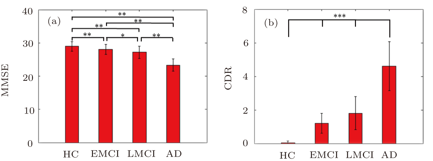
Fig. 1. (color online) Two sample t-tests of two kinds of cognitive scores between the four groups. The x axis represents HC, EMCI, LMCI, and AD groups, and the y axis indicates (a) MMSE score and (b) CDR score. The bar map indicates the mean values of cognitive scores among the four groups. The error bar represents the SD. *: P < 0.01, **: P < 0.005, and ***: P < 0.001. The asterisks indicate significant difference between groups.
Download figure:
Standard imageTable 1. Participant demographics and clinical information. In the table, the data are represented as mean ± standard deviation (SD). Columns on the right display P values of F-test for each sample characteristic except for gender, which displays the P value from a Chi-square test.
| HC | EMCI | LMCI | AD | P value | |
|---|---|---|---|---|---|
| Sample size | 51 | 75 | 39 | 48 | |
| Gender (male/female) | 26/25 | 49/26 | 25/14 | 28/20 | 0.400 |
| Age (years) | 72.68±6.16 | 72.96±8.04 | 72.83±5.72 | 74.59±9.01 | 0.563 |
| MMSE | 28.96±1.40 | 28.04±1.54 | 27.21±1.82 | 23.33±1.80 | < 0.01 |
| CDR | 0.03±0.12 | 1.21±0.60 | 1.81±0.98 | 4.62±1.46 | < 0.01 |
2.2. Data processing
The data preprocessing is performed by using PANDA (www.nitrc.org/projects/panda),[26] which is a pipeline toolbox for diffusion MRI analysis. PANDA is developed by applying the MATLAB software under an Ubuntu Operating System. A number of the processing functions from the FSL,[27] the Pipeline System for Octave and Matlab (PSOM),[28] Diffusion Toolkit,[29] and MRIcron software (http://www.mccauslandcenter.sc.edu/mricro/mricron/) are called by PANDA. Briefly, the preprocessing procedure includes skull-stripping, eddy-current, and head-motion correction, diffusion metrics calculation. FA, MD, AD, and RD maps in the MNI space are generated for each individual. Beyond that, Gong proposed a novel inter-voxel metric referred to as the local diffusion homogeneity (LDH).[30] This metric is defined to characterize the overall coherence of water molecule diffusion within a neighborhood, and can be used to explore inter-subject variability of WM microstructural properties. Computationally, the LDH metric uses Spearman's rank correlation coefficient (LDHs) or Kendall's coefficient concordance (LDHk) to quantify the overall coherence of the diffusivity series.
The diffusion metrics (i.e., FA, MD, DA, RD, LDHs, and LDHk) characterize microsturctural (e.g., degree of myelination or axonal organization) WM properties.[31] The regional values for these metrics are extracted using the White Matter Parcellation Map (WMPM), which is a prior WM atlas defined in the MNI space.[32] The mean of FA, MD, DA, RD, LDHs, and LDHk are calculated for each WMPM region. Here, a total of 50 WMPM regions are selected, and these areas are defined as the "core white matter".[32] The remaining peripheral WM regions near the cortex are excluded because they are highly variable across individuals.
2.3. Machine learning methods and analysis
A SVM method is applied to classify the four groups using diffusion metrics. The leave-one-out cross-validation (LOOCV) is adopted to evaluate the classification performance, which provides a good estimation for the generalizability of the classifiers, particularly when the sample size is small. Similarly, an LR method is reapplied to compare with the SVM method. All machine learning analyses are performed using Python (https://www.python.org/) and the tools are freely available at https://sourceforge.net/projects/scikit-learn.[33] The process flow chart of machine learning is shown in Fig. 2.

Fig. 2. (color online) The process flow chart in our work.
Download figure:
Standard image2.3.1. Feature combination
The data preprocessing can be seen in Fig. 2(a). Through the 50 WMPM atlas, we extract the regional values for different metrics. Then the six WM metrics (i.e., FA, MD, DA, RD, LDHs, and LDHk) for the 50 WMPM regions are concatenated to yield a single raw feature vector for each subject (Fig. 2(b)). A combination of multi-metric likely improves classification performance due to different metric could capture different aspects of WM tissue, which are potentially complementary for discrimination.
2.3.2. Feature selection
As is well known, the elimination strategy of the non-informative features is widely employed to enhance classification performance. A recursive feature elimination (RFE)[34] method combined with SVM or LR is applied in order to obtain an optimum feature dimension. The SVM-RFE or LR-RFE method allows one to minimize redundant and extraneous features which could potentially degrade classifier performance.[35] It works backwards from the initial set of features and eliminates the least "useful" feature on each recursive pass, and it had been applied successfully for feature selection in several functional neuroimaging studies.[36,37] Specifically, the process of feature selection is shown in Fig. 2(c). The x axis of the line chart represents the feature dimension, and the y axis indicates the classification score. The peak value marked with a red circle is the optimal feature dimension. Take SVM-RFE for example, the ranking criterion score of the i-th feature is defined as:

In each iteration, the feature with minimum ranking criterion score is removed and the remaining features are trained on the SVM classifier. The concrete algorithm of SVM-RFE is as follows:
Input: training samples {xi, yi}, yi ∈ {−1,1}.
Output: feature sorting set R.
(i) Initialization. Original feature set S = {1,2, ..., D}, feature sorting set R = Ø.
(ii) Loop through the following procedure until S = Ø:
ii-1) Acquisition of training samples with candidate feature sets;
ii-2) Receive ω according to Eq. (2):
where αi is the Lagrange multiplier and C is the penalty parameter.
ii-3) Calculate the ranking criterion score according to Eq. (1)

ii-4) find out the feature with minimum ranking criterion score

ii-5) Update the feature set

ii-6) Remove the feature among S

2.3.3. Classification
In terms of classification methods, SVM is by far the most popular method and is already known as a tool that discovers informative patterns.[34] The linear SVM with the LOOCV method is applied to implement the classification. Meanwhile, the logistic regression (LR),[38] another widely used classification model, is reapplied to validate the robustness of classification results via SVM. The classification diagram for the SVM classifier is shown in Fig. 2(d). Specifically, there exist training samples  where xi ∈ RD, yi ∈ {−1,1} is the class labels. N is the number of training samples, and D is the feature dimension of the sample. The goal of SVM is to explore the optimally classified hyperplane:

where w is the weight vector of the optimal hyperplane and b is the threshold value. This makes the optimally classified hyperplane not only separate the two kinds of samples accurately, but also maximize the classification interval between the two classes. The following optimization problem needs to be solved in order to obtain the weight vector and threshold vector:
where C > 0 is the penalty parameter and ξi is the slack variable. Parameter C plays a role in controlling the punishment degree of the misclassficaton, and realizes the tradeoff between the proportion of the wrong sample and the complexity of the algorithm. By introducing Lagrange multiplier, the optimization problem of SVM can be transformed into the dual programming problem as Eq. (2). The relationship between weight vector and dual optimization Eq. (2) is as follows:
The discriminant function of SVM is as follows:
where sgn(·) is the sign function.
Similar to the SVM method, the LR method also aims to obtain a linear classifier with a decision function y = f(x), in which y is the classification score and x is the multidimensional feature vector. The training and predicting framework is the same as the SVM method. In contrast, the LR method predicts the probability that a sample belongs to one class, rather than a hard label. The probability is defined as P = ey / (1 + ey), and the predicted label will be 1 (i.e., controls) if the probability is bigger than 0.5, otherwise −1 (i.e., AD). According to the algorithm implementation, the LR applies the maximum likelihood estimation to obtain the optimal classifier, rather than maximizing the margin as the SVM.
The principle of leave-one-out cross validation (LOOCV) method is as follows. Suppose there are N samples, each sample is taken as the test sample and the other N − 1 sample as the training sample. In this way, N classifiers and N test results are obtained. The average of these N results is used to measure the performance of the model.
2.3.4. Evaluation of classification performance
The results of classification are the accuracy, sensitivity, and specificity. Specifically, accuracy is the proportion of subjects who are correctly classified into group A or group B. Sensitivity and specificity are the proportion of group A and group B classified correctly. In order to understand the performance of a classifier, it is important to report the sensitivity or specificity along with the overall accuracy. The other very common way of reporting the sensitivity or specificity for a binary classifier is by plotting the "receiver operating characteristic" (ROC) curve.[39] The ROC curve is the plot of sensitivity against "1-specificity" by changing the discrimination threshold and therefore provides a complete picture of the classifier's performance. The ROC curve is usually summarized by the area under the curve (AUC), which is a number between 0 and 1.[39] Additionally, we apply a 1000 times permutation test without replacement to determine whether the actual accuracy is significantly higher than the values expected by chance. The p value for the accuracy is calculated by dividing the number of permutations that showed a higher value than the actual value for the real sample by the total number of permutations (i.e., 1000). At last, some discriminative features for each between-group comparison will be received after feature selection. A feature with higher weight represents a greater contribution to the classification.
3. Results
3.1. Cognitive performance
Since the machine learning methods used here are supervised learning, we need to know the label of each subject in advance, therefore the neuropsychological scale tests are essential. As is well known, psychometric analysis is applied to cognitive tests to improve their reliability, to allow the comparison of different cognitive tests, and to increase understanding of the cognitive processes underlying each test.
Based on the above purpose, we perform two sample T-tests on the cognitive score differences between different groups. The results are shown in Fig. 1. A decreasing MMSE score and increasing CDR score along with the severity of disease can be investigated obviously. The difference for MMSE score between the EMCI and LMCI group is less significant than that between other groups (P < 0.01). However, there are extremely significant differences in CDR scores among all four groups (P < 0.001). The above results are basically consistent with the statistical results in a recent review.[40]
The psychological scale of cognitive behavior is subjective and only used in patients with some clinical symptoms. In addition, once the symptoms have emerged and have been measured by the cognitive behavior scale, they have developed to the stage of disease. The effect has been very limited through medication and other therapeutics at this time. However, if we can find the effective markers in imaging diagnosis, we can intervene as early as possible.
3.2. Classification
The results shown in Table 2 have already experienced feature selection. The SVM and LR classifiers accurately discriminate the four groups using the single-type metric (FA, MD, DA, RD, LDHs, LDHk) and the combined metrics (Table 2). The classification accuracy here is significantly improved compared with previous research.[41–43] It seems that the combined metrics receive a better accuracy than the single-type metric. Notably, the SVM classifiers show a little advantage over the LR classifiers. To validate the robustness of the classification result, the permutation tests (1000 times) are applied in the combined metrics of between-group comparisons. The results show that the accuracies obtained above are significantly higher than values expected by chance (p < 0.001) except HC-EMCI comparison (p = 0.969) for LR.
Table 2. Classification performance for each kind of metric. All the numerical values in the table represent accuracy of percentage.
| SVM | |||||||
|---|---|---|---|---|---|---|---|
| Between-group comparison | FA | MD | DA | RD | LDHs | LDHk | Combined |
| HC versus AD | 87.88 | 84.85 | 91.92 | 89.90 | 91.92 | 90.91 | 89.90 |
| HC versus EMCI | 66.67 | 80.95 | 65.08 | 68.25 | 68.25 | 67.46 | 88.10 |
| HC versus LMCI | 80.00 | 83.33 | 72.22 | 71.11 | 86.67 | 87.78 | 100 |
| EMCI versus LMCI | 81.58 | 71.93 | 65.79 | 70.18 | 85.96 | 86.84 | 92.98 |
| EMCI versus AD | 78.05 | 78.86 | 77.24 | 74.80 | 77.24 | 74.80 | 84.55 |
| LMCI versus AD | 78.16 | 77.01 | 79.31 | 78.16 | 91.95 | 81.61 | 97.70 |
| LR | |||||||
|---|---|---|---|---|---|---|---|
| Between-group comparison | FA | MD | DA | RD | LDHs | LDHk | Combined |
| HC versus AD | 85.86 | 87.88 | 87.88 | 88.89 | 84.85 | 82.83 | 89.90 |
| HC versus EMCI | 62.70 | 69.04 | 68.25 | 66.67 | 73.81 | 65.08 | 64.30 |
| HC versus LMCI | 72.22 | 72.22 | 71.11 | 71.11 | 83.33 | 87.78 | 97.78 |
| EMCI versus LMCI | 70.18 | 67.54 | 69.30 | 71.05 | 77.19 | 76.32 | 88.60 |
| EMCI versus AD | 77.24 | 82.93 | 82.93 | 78.86 | 80.49 | 80.49 | 82.11 |
| LMCI versus AD | 73.56 | 79.31 | 79.31 | 80.46 | 79.31 | 81.61 | 95.40 |
The considerable classification accuracy among the compared groups can be well validated with the results of Fig. 1. Our results show that the majority of classifiers using combined metrics performed largely better than single WM metric-based classifiers, suggesting that all these features are jointly affected by AD. It should be noted that the discrimination performance using combined metrics only shows a slight improvement or even a trend compared with HC-AD comparison for SVM and HC-AD, HC-EMCI, and EMCI-AD comparisons for LR (Table 2). This may relate to the limited sample size or classification algorithm of this study, which requires future validation. Although the classification performances of a certain single-metric of certain between-group comparisons for the SVM classifier are worse than that of the LR classifier, the SVM classifier is better than the LR classifier for all between-group comparisons after metric combination, which also indirectly reflects that white matter damage is reflected on different levels. Moreover, it can be found that two novel metrics (i.e., LDHs and LDHk) also receive considerable accuracy, implying which may become imaging markers with great potential. In addition, the results of the permutation test also indirectly show the robustness of the classifiers (see Figs. 3 and 4).

Fig. 3. (color online) The histograms of permutation distribution of the accuracy for SVM classifier.
Download figure:
Standard image
Fig. 4. (color online) The histograms of permutation distribution of the accuracy for LR classifier.
Download figure:
Standard image3.3. Evaluation of classifier performance
The application of ROC curve analysis in the evaluation of diagnostic testing has been more and more widely accepted, and has become the standard statistical method of clinical screening and diagnostic evaluation at home and abroad.[44] The greatest characteristic of ROC curve analysis is the integration of sensitivity and specificity into one index, which is not affected by the incidence of disease. This characteristic is beneficial for both diagnosis and elimination of disease.[45] The essence of ROC curve analysis is to analyze its sensitivity and specificity under multiple diagnostic thresholds.[46] These ROC curves and AUCs (Fig. 5) show the classifiers' performance for combined metrics of all between-group comparisons. It can be found that the use of SVM classifiers generally obtain better performance than that of LR classifiers. It seems that the robustness of HCs versus EMCIs is not superior to that of other groups, possibly because the EMCIs marker on brain imaging is similar to that of HCs, even though they exhibit difference in cognitive function. Notably, the above results indirectly reflect the sensitivity and specificity of classifiers. Therefore, the ROC curves and AUCs can be validated by the classification performance of combined multi-type WM metrics and reflected the sensitivity and specificity of the classifiers.

Fig. 5. (color online) The ROC curves and AUCs for different between-group comparisons of SVM classifiers and LR classifiers to evaluate classifier output quality using twenty-fold cross-validation. Different colors of full line represent different between-group comparisons.
Download figure:
Standard image3.4. Discriminative WM features
To further illustrate the importance of different WM tract to classification, the top 10 features with higher weight are selected for each between-group comparison. Meanwhile, the best feature dimensions are shown in Table 3. For any features which appear repeatedly in multiple between-group comparisons, we consider them as the most important features which contribute to classification. Statistically, these features are uncinate fasciculus, cingulum, superior corona radiate, external capsule, internal capsule, corpus callosum, and pontine crossing tract, respectively.
Table 3. The discriminative features of SVM classifier. In the table letter "L" means left, "R" means right.
| WMPM regions | Metric | WMPM regions | Metric |
|---|---|---|---|
| (AD versus EMCI: 143) | (AD versus LMCI: 120) | ||
| Retrolenticular part of internal capsule (R) | FA | External capsule (L) | FA |
| Uncinate fasciculus (L) | RD | External capsule (L) | RD |
| Cingulum hippocampus (L) | LDHk | Splenium of corpus callosum | LDHk |
| Retrolenticular part of internal capsule (L) | DA | Middle cerebellar peduncle | LDHs |
| Superior corona radiata (R) | LDHk | Splenium of corpus callosum | LDHs |
| Tapetum (R) | FA | External capsule (L) | MD |
| Superior corona radiata (R) | LDHs | Medial lemniscus (R) | FA |
| Inferior fronto-occipital fasciculus (L) | FA | Retrolenticular part of internal capsule (R) | DHk |
| Uncinate fasciculus (L) | MD | Genu of corpus callosum | LDHk |
| Cingulum (cingulate part) (R) | DA | Genu of corpus callosum | LDHs |
| WMPM regions | Metric | WMPM regions | Metric |
|---|---|---|---|
| (AD versus NC: 232) | (EMCI versus NC: 163) | ||
| Pontine crossing tract | DA | Pontine crossing tract | RD |
| Cingulum hippocampus (L) | FA | Pontine crossing tract | MD |
| External capsule (L) | FA | Cingulum (cingulate part) (R) | DA |
| Splenium of corpus callosum | LDHk | Cingulum hippocampus (R) | LDHs |
| Splenium of corpus callosum | LDHs | Cerebral peduncle (R) | LDHk |
| Crus of fornix (L) | FA | Cingulum hippocampus (L) | DA |
| Cingulum hippocampus (R) | FA | Cingulum hippocampus (R) | LDHk |
| Superior corona radiata (L) | FA | Uncinate fasciculus (R) | LDHs |
| Anterior limb of internal capsule (L) | FA | Superior corona radiata (R) | LDHk |
| External capsule (L) | RD | Anterior limb of internal capsule (L) | DA |
| WMPM regions | Metric | WMPM regions | Metric |
|---|---|---|---|
| (LMCI versus EMCI: 25) | (LMCI versus NC: 94) | ||
| Middle cerebellar peduncle | LDHs | Middle cerebellar peduncle | LDHs |
| Body of corpus callosum | LDHk | Pontine crossing tract | LDHk |
| External capsule (L) | LDHs | Cingulum hippocampus (L) | MD |
| Superior longitudinal fasciculus (L) | LDHs | Anterior corona radiata (R) | LDHk |
| Superior cerebellar peduncle (L) | DA | Cingulum hippocampus (L) | DA |
| Cingulum (cingulate part) (R) | LDHs | Cingulum hippocampus (L) | RD |
| Anterior corona radiata (L) | LDHs | Pontine crossing tract | LDHs |
| Superior fronto-occipital fasciculus (R) | LDHk | Middle cerebellar peduncle | LDHk |
| Superior corona radiata (L) | RD | Body of corpus callosum | FA |
| Cingulum hippocampus (L) | RD | Uncinate fasciculus (L) | FA |
The limbic system and association fiber were the abnormal areas that were being most reported in WM research of AD.[47–49] Cingulum is the important associative fiber that was tight related with episodic memory between cingulate gyrus and other brain GM structures. An impaired cingulum would lead to interruption of hippocampus and cerebral cortex, even causing dysmnesia in AD patients. Bozoki and colleagues[50] revealed that descending cingulum integrity declined during both the transition from normal aging to MCI and the transition from MCI to AD. This research strongly verified that the cingulum played an important role in between-group classification. The corpus callosum is a thick plate of fibers that reciprocally interconnected the left and right hemisphere. According to previous studies, the anterior part of the corpus callosum contained interconnecting fibers that associated with the feeling of motivation were from the prefrontal cortex.[51] Furthermore, the deficiency of the corpus callosum integrity might lead to slow initiation and longer reaction times in ADs. Bozzali and colleagues[52] discovered a notable decrease of the corpus callosum area from ADs compared with age matched healthy subjects. The aforementioned research illustrated the corpus callosum is an importance WM tract for revealing the developmental stage of AD. Moreover, the relevant studies indicated that AD was associated with changes in the WM of the frontal and temporal lobes.[53,54] The uncinate fasciculus is a white matter tract that connects the anterior part of the temporal lobe and is considered to play a role in emotion, decision-making, and episodic memory.[55,56] Review of many experimental studies supported the role of the uncinate fasciculus whose disruption resulted in severe memory impairment.[55,57] The disruption in connectivity between the temporal and frontal lobes via the uncinate fasciculus was postulated as a possible cause of posttraumatic retrograde amnesia.[55,58] The internal capsule is the major route that connects with the brainstem and spinal cord and contains both ascending and descending axons. Moreover, the internal capsule contains the pyramidal tracts, which imply its effect in somatic movement. It is likely that the impairment of an internal capsule would lead to movement disturbance in AD. The corona radiata, as the most prominent projection fiber, radiates out from the cortex and comes together in the brain stem, which continue ventrally as the internal capsule. Corona radiata is related to the motor pathway and speculative analysis so that the AD or MCI patients would suffer motor and cognitive dysfunction.[59] The external capsule and uncinate fasciculus comprise the capsular division of the lateral cholinergic pathway. The capsular division of the lateral cholinergic pathway innervates frontal, parietal, and temporal neocortices.[60] The damage in the lateral cholinergic pathway is consistent with AD pathology. The above research demonstrated the corona radiate, external capsule, and internal capsule are important WM features for classification in our research.
4. Conclusion and perspectives
The present work applies six kinds of WM metrics and two classification methods to identify HC, EMCI, LMCI, and AD. To the best of our knowledge this is the first time LDHs and LDHk have been used as novel classification metrics. Additionally, the uncinated fasciculus, cingulum, corpus callosum, corona radiate, external capsule, and internal capsule are considered to be distinguishing features for classification of between-group. The promising results indicate that multi-type and multi-regional brain WM features can effectively improve the accuracy of diagnosis for AD and MCI. This study demonstrates that AD or MCI can be distinguished from HC by jointly using multi-type and multi-regional WM features, indicating a multidimensional impairment existed in AD. Notably, a set of discriminative features are consistently recognized using two distinct classification models (i.e., SVM and LR). These WM results commendably illuminate the neural mechanisms underlying AD. Finally, the proposed WM imaging-feature-based classification method for AD implies an alternative way for identifying Alzheimer's individuals, which offers a valuable clue in clinical diagnosis.
The importance of our study can be summarized in four points. (I) Except the familiar diffusion metrics FA, MD, DA, and RD, we add the LDHs and LDHk diffusion metrics for multi-metric analysis. (II) The MCI is divided into EMCI and LMCI to further validate the classification capacity of the classifier. (III) Except single diffusion metric classification, we combine the multi-type and multi-regional metrics together for improving classification performance. (IV) The discriminative features for classification are listed to show the importance of different WM fiber tracts. There are several limitations in this study. First, the results may be unreliable by the relatively small sample size. Although our results successfully classify the four groups using a machine learning model, further validation on a larger sample is required to understand the present results. Second, longitudinal studies should be conducted to clarify the progression of brain changes over time. Finally, many factors such as brain atrophy, hyper-intensity, and between-subject misalignment due to registration errors may distort the values of diffusion metrics. To avoid this, more advanced imaging techniques and sophisticated algorithms are desired.
Footnotes
- *
Project supported by the National Natural Science Foundation of China (Grant No. 11572127).