

Abstract
Cepheid variable stars calibrate the cosmic distance ladder and exhibit large-amplitude pulsations that provide interesting hydrodynamical insights into stellar atmospheres. Here, we investigate velocities of different spectral line species (ionization levels, elements) to provide new detail into the complex velocity structure of the particularly large-amplitude Cepheid X Cygni, Ppuls = 16.3 d. This is done against the backdrop of studies aimed at understanding the projection factor for Baade-Wesselink-type distance methods, as well as the timeseries velocimetry being gathered by the Gaia satellite. We analyze and compare velocities measured by cross-correlation using thousands of optical metallic lines, as well as individual line velocities of hydrogen (Balmer and Paschen lines), oxygen, ionized silicon, potassium, sodium, and ionized calcium. We compare individual line velocity curves to a reference velocity curve based on cross-correlation and discuss observed differences as a function of pulsation phase. This purely empirical approach yields detailed insights into the dependence of certain lines on NLTE effects, shocks, and phase lags in velocity space, which can be used as strong constraints for hydrodynamical modeling. Of particular importance is the velocity curve of the Ca II IR triplet, which dominates the Gaia radial velocities of F, G, and K type variable stars.
Export citation and abstract BibTeX RIS
1. Introduction
While Cepheid variables have usually been studied for their influence on the calibration of the distance scale to nearby galaxies, they are also interesting as testbeds for the complex interactions of hydrodynamics, thermodynamics, and radiative transfer. Efforts to understand the kinematics of Cepheid atmospheres date back to the first radial velocity (RV) curves by (Belopolsky 1895, 1897), who showed that the relationship between timing of the light and velocity changes contradicted the then accepted model of eclipses. More recently, Herbig (1952), Kraft (1956), Greenstein (1960) and Butler et al. (1996) have shown how complicated are the atmospheres of Cepheids with periods longer than about 10 days. Petterson et al. (2005) observed 14 Cepheids with periods from 2 to 35 days using a spectroscopic resolution of 27 000, and very good phase coverage, for the purpose of recognizing the dependence of velocity with depth of line formation. Sasselov (1989); Nardetto et al. (2007), and Hadrava et al. (2009) analyzed Cepheids in terms of the depth of line formation and the excitation of their lower levels of absorption lines.
As a follow-up to Kraft's 1956 paper and his measured velocities for Hα (displayed by Greenstein 1960), one of us (G.W.) obtained new velocity curves for Cepheids, including the long-period stars X Cyg (Wallerstein 1983), T Mon (Wallerstein 1972), and SV Vul (Grenfell & Wallerstein 1969). Those velocity curves were all recorded on photographic plates and, hence, did not include wavelengths beyond about 6800 Å. With modern CCD detectors, the wavelength coverage has been extended to 10 200 Å to include the O I triplet at 7771,4,5 Å, the IR Ca II triplet, and several Paschen lines. The inclusion of the Paschen lines allows a comparison with the Balmer lines, which are of particular interest because of the suggested overpopulation of the 2 s level of hydrogen due to the fact that the 2s → 1s transition is strongly forbidden (Struve et al. 1939). The near-IR velocity curve has been described by Butler & Bell (1997).
In this second paper in our series on individual line velocities of various species (Wallerstein et al. 2015, Paper I), we present phase-resolved line velocities for the long-period, high-amplitude Cepheid X Cygni. We focus on an empirical description of the atmospheric dynamics of lines affected by NLTE and/or formed over a significant range in optical depth, and consider differences between velocities measured using different techniques in the context of the ESA Gaia survey, which is measuring RVs using the IR Ca II triplet (Munari 1999). Specifically, we discuss the difference in projection factor required when measuring RVs using the IR Ca II triplet (as Gaia does), and the more commonly found velocities determined by cross-correlation of thousands of optical metallic spectral lines.
Recent detections of Cepheids with radio telescopes, Chandra, and XMM-Newton (Engle et al. 2014, 2017; Evans et al. 2016) have shown that there are phenomena in the outer layers of Cepheids that must be initiated by observable phenomena in their atmospheres.
The paper is structured as follows: we describe the observations and data treatment in Section 2. Section 3 describes the average metallic line RV curve measured by cross-correlation, which provides a contemporaneous ephemeris and velocimetric reference for the individual line velocities presented in Section 4. Section 5 discusses the challenges and opportunities of measuring individual line velocities in Cepheids.
2. Observations
We have two new sources of data for X Cygni. 24 spectra were obtained with the echelle spectrograph on the 3.5-m telescope at the Apache Point Observatory (APO) in Sunspot, New Mexico. They are recorded on a Site-2 CCD with a resolving power of ∼30 000, and wavelength coverage from 10 200 Å to 3600 Å. Since the sensitivity of the CCD peaks around 7000 Å, and Cepheids are fairly red, the spectra are most useful in the 4100–10 200 Å range, i.e., from Hδ to just beyond the Paschen-δ line at 10 049 Å. The spectra were reduced with standard processes in IRAF and calibrated for wavelength with a ThAr arc. The wavelengths of the atmospheric O2 absorption lines in the 7600–7700 region were measured and found to fall within 0.1 or 0.2 Å of their tabulated values. Measurements were made using the "k" command in the SPLOT routine, which fits the observed line with a Gaussian approximation between specified wavelengths. This procedure is very effective in deriving the wavelength of symmetric lines, but does not account for line asymmetry or complex line shapes, such those exhibited by Hα.
We further obtained 40 high-resolution (R∼85 000) spectra using the Hermes spectrograph mounted on the Flemish 1.2 m Mercator telescope located on the Roque de los Muchados Observatory on La Palma, Canary Island, Spain (Raskin et al. 2011). The wavelength scale was obtained via a ThArNe reference spectrum. One spectrum was obtained on 2010 November 15, 15 spectra between June and 2015 September 2015 between 2016 June and September, and 10 between 2017 September and November using the high-resolution fiber (HRF) mode for best resolving power and throughput. All of the Hermes spectra were processed by the reduction pipeline, which includes standard processing steps such as flatfielding, bias corrections, order extraction, and cosmic clipping (cf. also Anderson et al. 2015). These spectra were obtained with the goal of determining RVs via the cross-correlation technique. The median signal-to-noise (S/N) of these spectra is approximately 50 near 6000 Å, and the useful wavelength range is from 9000 Å down to Hβ. Individual line velocities were measured on the 2014 and 2015 Hermes data to supplement phase coverage, despite the lower-than-desired S/N ratio.
The photographic plates commonly used in the 1980 s had a resolution of 20 microns, which was significantly better than the 2, 24 micron pixel resolution of the site-2 CCD that was used in the APO echelle spectra.
In order to examine the behavior of X Cyg's atmosphere during the critical phase of rising light when the velocity is rapidly decreasing we concentrated observations on that part of the pulsation cycle. The light and B–V color curves are shown in Figure 1.

Figure 1. AAVSOnet Epoch Photometry Data (v1.0) V–band and B–V color photometry of X Cygni. The data shown were observed using the AAVSO Bright Star Monitors BSM-HQ and BSM-NM and phase-folded using the ephemeris mentioned in Section 3.
Download figure:
Standard image High-resolution image3. The Velocity Curve Based on Cross-correlation
We measure high-precision velocities of X Cyg by cross-correlating the optical spectral range with an input numerical mask containing 1130 spectral lines and fitting a Gaussian to the resulting cross-correlation function (CCF) (Baranne et al. 1996). Uncertainties are assigned based on the fit agreement between the computed cross-correlation profile and the Gaussian profile, and are computed using the Hermes pipeline (Raskin et al. 2011). As part of our observing strategy, we recalibrate the wavelength solution whenever changes in the atmospheric pressure may lead to drifts in RV zero-point ∼50 m s−1. Further corrections for RV effects due to changes in ambient pressure maintain a zero-point stable to about 15 m s−1 (Anderson 2013; Anderson et al. 2015). The somewhat conservative median RV uncertainty is 71 m s−1.
In the following, we use the Hermes cross-correlation RV (CC RV) curve as a reference for comparison with other velocities. Defining ϕ = 0 at minimum velocity, we find Ppuls = 16.38615d and Eref = 2 457 349.31541. Figure 2 shows the phase-folded CC RV curve as well as the residuals obtained by subtracting a Fourier series with 11 harmonics and mean velocity vγ,CC = 9.616 km s−1. The peak-to-peak RV amplitudes defined by the (discrete) observations and the (continuous) Fourier series model are 54.499 km s−1 and 54.673 km s−1 respectively.7
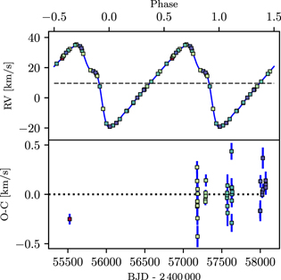
Figure 2. Radial Velocity curve of X Cygni based on a cross-correlation of Hermes optical spectral orders and 1130 spectral lines. Top: phase-folded RV curve, bottom: Residuals after subtracting a Fourier series model using 11 harmonics.
Download figure:
Standard image High-resolution imageWe find no clear indication of cycle-to-cycle RV curve modulation (Anderson 2014) based on the Hermes data alone. This is not surprising, since the phase coverage of the present data is not particularly dense (in each cycle), and since possible short timescale fluctuations in pulsation period further complicate the distinction in case of a weak modulation. We do note, however, that the rms around the Fourier series is 0.16 km s−1, i.e., 2.3 times larger than the median uncertainty. Literature RVs spanning a longer baseline exhibit some differences at the 1–2 km s−1 level (Kiss 1998; Gorynya et al. 1992; Bersier et al. 1994; Storm et al. 2004; Barnes et al. 2005), notably near the lower part of the RV curve, which could potentially indicate a slow amplitude change or zero-point differences among the measurements (Anderson 2018). Older, less precise, RV data (Barnes et al. 1987; Wilson et al. 1989) also generally agree with vγ defined by the Hermes measurements. Hence, we find no clear evidence of a spectroscopic orbital signature (with semi-amplitude K >1 km s−1) via systematic variations in vγ over a baseline of 40.5 yr.
As shown by contemporaneous photometry obtained by AAVSOnet, ϕ = 0 of the RV CC data coincides rather well with maximum light, cf. Figure 1. The AAVSOnet photometry and Hermes RV CC curve are partially contemporaneous, with mean HJDs of 2 456 754.4 for the photometry and 2 457 342.3 for the Hermes data.
In the following, we use the CC RV curve as a baseline for comparisons with velocities of more restricted wavelength ranges or individual lines.
4. Individual Line Velocity Curves
It has been known for a long time that different spectral lines exhibit velocity differences owing to the presence of velocity gradients in pulsating stellar atmospheres (Kraft 1957 and Mathias & Gillet 1993). This section presents RVs determined on either individual spectral lines, or groups of lines of similar nature, providing a more detailed description of atmospheric dynamics, as well as a comparison of velocity amplitudes with the CC RV reference. Table 1 lists the dates, phases, and velocities measured using all of our spectra.
Recently, Anderson (2016) has shown that velocity gradients are subject to modulation, leading to cycle-dependent distortions of spectral line profiles at a given phase. For individual line velocities, we cannot hope to detect such cycle-to-cycle modulations due to a lack of precision for the individual velocity estimates. Therefore, the following description is limited to the assumption of a perfectly repeating behavior.
Table 1. Individual Line Radial Velocity Measurements in km s−1 Based on APO and Hermes Spectra
| HJD | ϕ | Inst | Pa H | O I | K I | Si II | Na I | Hα | Hβ | Hγ | Hδ | Ca IIIR | Ca IIV | Fe/Ti I | Fe/Ti II |
|---|---|---|---|---|---|---|---|---|---|---|---|---|---|---|---|
| 57185.55 | 0.006 | HER | −16.62 | −19.33 | −10.81 | −18.51 | ⋯ | −49.16 | 5.23 | −18.41 | −20.02 | −31.61 | 29.04 | ⋯ | ⋯ |
| 56350.00 | 0.016 | APO | −19.13 | −20.78 | −16.18 | −21.03 | −18.48 | 35.64 | −12.58 | −18.98 | −20.08 | −36.28 | −18.18 | −23.63 | −19.48 |
| 56087.98 | 0.026 | APO | −18.34 | −10.44 | −11.64 | −10.54 | −13.84 | −28.34 | −17.14 | −20.44 | −26.34 | −36.98 | ⋯ | −11.14 | −12.74 |
| 57186.55 | 0.067 | HER | −16.09 | −16.60 | −10.80 | −16.09 | ⋯ | −57.49 | −37.68 | ⋯ | −31.59 | −37.44 | 2.90 | ⋯ | ⋯ |
| 56088.91 | 0.083 | APO | −14.94 | −15.61 | −13.61 | −15.66 | −14.01 | −3.11 | −17.11 | −20.41 | −26.71 | −35.41 | ⋯ | −14.81 | ⋯ |
| 56383.93 | 0.086 | APO | −17.65 | −16.60 | −14.20 | −17.45 | −15.25 | −52.50 | −20.70 | −31.70 | −36.70 | −34.20 | ⋯ | −20.10 | −20.10 |
| 56630.52 | 0.135 | APO | −8.60 | ⋯ | ⋯ | ⋯ | ⋯ | −36.50 | −22.20 | −19.20 | −21.40 | ⋯ | ⋯ | ⋯ | ⋯ |
| 56630.52 | 0.135 | APO | −7.70 | −10.30 | −9.90 | −10.80 | −11.60 | −42.30 | −27.30 | −22.70 | −22.20 | −27.80 | −31.60 | −12.50 | −18.50 |
| 56466.95 | 0.153 | APO | −10.43 | −10.93 | −11.13 | −11.03 | −12.73 | 5.07 | −8.73 | −21.83 | −22.13 | ⋯ | ⋯ | −12.13 | −10.83 |
| 57286.42 | 0.162 | HER | −9.68 | −8.04 | −9.10 | −7.73 | −10.61 | −45.47 | −30.97 | −20.12 | −18.70 | −17.52 | 28.39 | ⋯ | ⋯ |
| 57287.37 | 0.220 | HER | −6.13 | −2.77 | −5.50 | −2.30 | −8.01 | −42.54 | −25.41 | −14.12 | −16.17 | −12.49 | 2.58 | ⋯ | ⋯ |
| 57289.44 | 0.346 | HER | 7.27 | 8.15 | 7.57 | 8.29 | 6.35 | 19.96 | −20.10 | −15.97 | ⋯ | −1.17 | ⋯ | ⋯ | ⋯ |
| 57291.36 | 0.463 | HER | 22.43 | 16.55 | 17.58 | 17.31 | 18.92 | 14.73 | 7.09 | ⋯ | ⋯ | 11.89 | 28.03 | ⋯ | ⋯ |
| 55523.42 | 0.573 | HER | 27.95 | 25.22 | 25.81 | 24.08 | 28.76 | 10.19 | 11.87 | ⋯ | ⋯ | 23.78 | 69.92 | ⋯ | ⋯ |
| 57178.58 | 0.581 | HER | 29.13 | 27.10 | 27.45 | 25.13 | 29.95 | 8.73 | ⋯ | ⋯ | ⋯ | 23.83 | ⋯ | ⋯ | ⋯ |
| 57293.42 | 0.589 | HER | 32.70 | 26.93 | ⋯ | 27.10 | 31.10 | 9.10 | 16.44 | ⋯ | ⋯ | 27.03 | 7.78 | ⋯ | ⋯ |
| 56375.94 | 0.599 | APO | 23.43 | 24.83 | 26.23 | 22.93 | 28.08 | 11.03 | 17.23 | 21.63 | 21.23 | 25.73 | −3.57 | 26.03 | 26.33 |
| 56441.89 | 0.624 | APO | 27.03 | 27.73 | 30.83 | 27.43 | 33.33 | 5.63 | 20.13 | ⋯ | ⋯ | 29.13 | ⋯ | 29.43 | 33.13 |
| 57179.59 | 0.642 | HER | ⋯ | 30.70 | 32.58 | 29.52 | 35.44 | 8.44 | 20.08 | ⋯ | ⋯ | 32.50 | 30.15 | ⋯ | ⋯ |
| 56098.96 | 0.696 | APO | 29.69 | 33.54 | 36.64 | 32.44 | 41.34 | 3.64 | ⋯ | ⋯ | ⋯ | 39.84 | 9.04 | 37.24 | 42.94 |
| 57180.58 | 0.703 | HER | 37.33 | 32.81 | 35.96 | 31.18 | 40.16 | 9.27 | 28.61 | ⋯ | ⋯ | 39.80 | −3.29 | ⋯ | ⋯ |
| 56099.95 | 0.757 | APO | 25.89 | 27.29 | ⋯ | 25.66 | 38.60 | 4.99 | ⋯ | ⋯ | ⋯ | 39.29 | 38.89 | 28.89 | 34.24 |
| 57181.59 | 0.764 | HER | 29.40 | 27.68 | 29.90 | 26.49 | 39.15 | 10.75 | 37.59 | ⋯ | ⋯ | 48.09 | 43.08 | ⋯ | ⋯ |
| 55903.52 | 0.769 | APO | 24.06 | 27.01 | ⋯ | 25.91 | 38.71 | 11.01 | 38.11 | 64.11 | ⋯ | 49.61 | −7.89 | 28.61 | 36.61 |
| 55903.52 | 0.769 | APO | ⋯ | 27.21 | 28.61 | 24.61 | 39.01 | 12.31 | 37.91 | ⋯ | ⋯ | 50.21 | ⋯ | 29.31 | 35.31 |
| 55903.53 | 0.770 | APO | 31.50 | 28.20 | 28.60 | 22.60 | 39.20 | 38.10 | 38.10 | 38.10 | 38.10 | 49.80 | −9.70 | 30.90 | 33.60 |
| 56477.93 | 0.823 | APO | 6.81 | 17.41 | 18.11 | 15.11 | 18.91 | 7.51 | 38.01 | ⋯ | ⋯ | 49.01 | ⋯ | 15.11 | 17.26 |
| 55904.52 | 0.830 | APO | 18.01 | 19.61 | ⋯ | 19.41 | 24.81 | 12.11 | 40.11 | ⋯ | ⋯ | 51.51 | −54.69 | 19.91 | 20.91 |
| 55904.53 | 0.831 | APO | 18.49 | 19.09 | 18.49 | 19.09 | 23.39 | 12.09 | 35.59 | ⋯ | 22.89 | 47.69 | −7.81 | 18.39 | ⋯ |
| 57182.68 | 0.831 | HER | 20.76 | 18.85 | 17.25 | 18.89 | 19.84 | 10.55 | 38.66 | 57.08 | 32.91 | 46.51 | ⋯ | ⋯ | ⋯ |
| 57183.57 | 0.885 | HER | 16.49 | 15.30 | 16.03 | ⋯ | 18.05 | 13.48 | 32.25 | ⋯ | ⋯ | 39.13 | 56.59 | ⋯ | ⋯ |
| 57183.68 | 0.892 | HER | 17.56 | 14.43 | 15.29 | 14.52 | 17.22 | 15.91 | 31.54 | 24.92 | 18.44 | 35.21 | 38.21 | ⋯ | ⋯ |
| 55905.58 | 0.895 | APO | 12.38 | 10.63 | 13.63 | 12.73 | 22.83 | 10.53 | 38.83 | 24.43 | 10.43 | 47.23 | −13.07 | 10.03 | 11.13 |
| 57184.55 | 0.945 | HER | −4.36 | −5.96 | −8.64 | −6.99 | ⋯ | 19.55 | 24.66 | 21.40 | 6.77 | 35.43 | 29.22 | ⋯ | ⋯ |
| 55906.52 | 0.952 | APO | −7.08 | −12.18 | −12.38 | −11.78 | −9.58 | 33.12 | 23.62 | 19.12 | 4.82 | 31.62 | ⋯ | −12.68 | −10.68 |
| 56381.92 | 0.964 | APO | −13.57 | −17.87 | −14.67 | −17.47 | −14.97 | 31.03 | 17.53 | 12.73 | 20.53 | −11.27 | ⋯ | −21.47 | −18.47 |
| 56463.97 | 0.971 | APO | −12.96 | −16.36 | −12.56 | −16.16 | −12.76 | 26.54 | ⋯ | ⋯ | ⋯ | 29.54 | ⋯ | −19.16 | −16.26 |
| 56644.52 | 0.989 | APO | −15.59 | −16.09 | −11.39 | −16.89 | −11.99 | 39.31 | 15.11 | −6.39 | −14.49 | −25.79 | −6.19 | −19.89 | −17.19 |
Note. Pulsation phase ϕ is computed using the Hermes cross-correlation RV curve so that  at minimum RV. All velocities have been corrected for the barycentric Earth radial velocity (BERV).
Download table as: ASCIITypeset image
4.1. Uncertainty Estimation of Individual Line Measurements
It is not easy to estimate the uncertainty of each velocity measurement as some features are represented by only one or two lines in each spectrum. However, the APO spectral resolution of 10 km s−1 and S/N of near 100 (though somewhat lower below 4500 Å), provide line profiles that mimic Gaussians, or have Gaussian cores in the case of the strongest lines. Hence, we have used the k command in the SPLOT package of IRAF to estimate the central wavelength of each line. To test the precision of the derived velocities, we obtained five consecutive exposures of 2 minutes, each on 2015 March 9 and measured all of them in one afternoon. Table 2 shows the standard error of the mean. Some lines that appear in two orders of the echelle spectrum were measured twice if they were not too close to the noisy edge of the order. Except for Hα, all lines were present only in absorption. The broader lines of H and K Ca II show larger uncertainties than the neutral and ionized lines of other species.
Table 2. Error Estimates for Five Near-simultaneous Measurements
| Species | Lines (Å) | V (km s−1) | N | σerr (km s−1) |
|---|---|---|---|---|
| Hαem | 6562.81 | 20.10 | 8 | 0.57 |
| Hαab | 6562.81 | 89.76 | 8 | 1.20 |
| Hβ, γ, δab | 4101.73, 4340.46, 4861.33 | −19.25 | 21 | 5.20 |
| Paschen | 8502.48, 8598.39, 8750.47, 8862.78, 10 049.48 | −8.21 | 24 | 9.30a |
| Fe I | 6703.57, 6705.11, 6710.31, 6717.55 | −6.10 | 19 | 2.50 |
| Si II | 6347.09, 6371.35 | −7.91 | 10 | 0.91 |
| Na I | 5889.95, 5895.92 | −14.10 | 10 | 0.29 |
| K I | 7698.97 | −9.65 | 5 | 0.21 |
| O I | 7771.96, 7774.18, 7775.40 | −7.50 | 15 | 0.35 |
| Ca II | 8498.02, 8542.09, 8662.14 | −17.93 | 18 | 2.70 |
Note.
aThe high uncertainty in the Paschen line velocities is due to the first four lines, which are blended with other stellar and atmospheric lines. The 10 049 Å line was not included in the Hermes spectra.Download table as: ASCIITypeset image
Table 3. Results From Fitting the RV Curve Template Based on Hermes CC RVs to Individual Line Velocities
| Line | Δϕb | Δϕt |

|
Δvr,min | Δvr,max | Δvγ |
|---|---|---|---|---|---|---|
| Hβ | −0.0832 | −0.1392 | 10.14 | −7.81 | 2.33 | 1.4 |
| Hγ | −0.0594 | −0.0950 | 9.29 | −7.80 | 1.49 | −13.2 |
| Hδ | −0.0508 | −0.0729 | 5.84 | −9.18 | −3.34 | −14.4 |
| Ca II IR | −0.0325 | −0.1313 | 26.27 | −14.26 | 12.01 | 6.9 |
| Pa H | −0.0045 | 0.0063 | 0.51 | −0.20 | 0.31 | −1.3 |
| O I | 0.0031 | −0.0003 | −1.50 | 0.26 | −1.24 | −1.3 |
| Fe II/Ti II | −0.0009 | −0.0100 | 3.59 | −1.67 | 1.92 | −1.9 |
| Ba II | −0.0120 | −0.0181 | 3.22 | −2.57 | 0.65 | −3.1 |
| Si II | 0.0034 | 0.0020 | −2.27 | 0.13 | −2.14 | −2.1 |
| Fe I/Ti I | 0.0075 | −0.0023 | 0.55 | −1.43 | −0.88 | −4.6 |
| Na I | −0.0051 | −0.0206 | 3.28 | 0.39 | 3.67 | 4.5 |
| K I | 0.0057 | −0.0017 | −1.66 | 1.55 | −0.12 | −1.9 |
Note. Phase offsets near the line velocity's minimum (Δϕb) and maximum (Δϕt) were determined separately. Negative Δϕ indicates that the minimum RV of the CC curve occurs before the individual line RV curve.  denotes the difference in peak-to-peak RV variation, and Δvr, the differences near RV curve maximum and minimum. Δvγ =
  is the difference in average velocity defined by the constant term of the CC RV Fourier series fit and the mean of a given line's RV timeseries.
Download table as: ASCIITypeset image
The Paschen velocities are somewhat more uncertain than the APO velocities because the 10 049 Å line was not covered in the Hermes spectra.
Table 4. Velocity Amplitudes of Various Species
| Species | Amplitude (km s−1) |
|---|---|
| CC Curve | 54.50 |
| 4500–4600 Å metallic lines | 63.04 |
| O I | 81.02 |
| Si II | 79.06 |
| Hβ | 85.89 |
| Hγ | 75.39 |
| Hδ | 64.27 |
| Pa H | 81.05 |
| Ca II | 97.57 |
| Na I | 49.11 |
| K I | 73.09 |
Download table as: ASCIITypeset image
4.2. Metallic Line Radial Velocities
Figure 3 shows the velocity curve derived from metallic lines in the 4500–4600 Å region using the APO spectra. Most of the lines are from Ti I, Ti II, Cr I, Cr II, Fe I, and Fe II. As the bottom panel shows, the agreement between both data sets is quite good. Unsurprisingly, the CC RV curve has much lower scatter than the RVs based on this more narrow wavelength range due to the much increased S/N of the CC profile covered to individual line profiles.
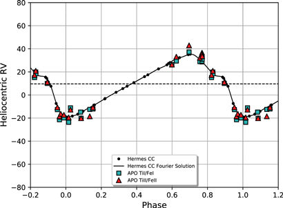
Figure 3. Metallic Line Velocity Curve.
Download figure:
Standard image High-resolution image4.3. The Hydrogen Lines
The profiles of the Hα line exhibit exceedingly complex variations during a pulsation cycle. For most other species, it is not difficult to measure the radial velocity of each absorption line, however, the complex asymmetric and phase-dependent structure of the Hα profile makes it impossible to assign a single number to characterize the velocity of the line. Clearly, the entire line profile needs to be modeled by the moving atmosphere. The line profile variations of Hα and their relation to shocks in X Cygni's atmosphere has already been described in great deal (Gillet 2014), so this is not deemed necessary here. We illustrate the difference in line profiles of the Balmer and Paschen lines in Figure 4, where we show a side-by-side comparison between the Hα and the Paschen-λ 8862.79 Å lines from Hermes spectra as they change during the pulsation cycle.
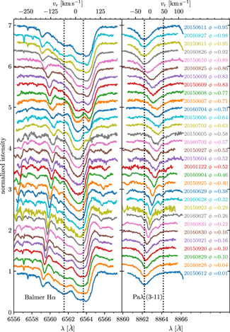
Figure 4. Profiles of the Hα and Paschen-α line at 8862 Å as observed by Hermes. The vertical dotted lines indicate minimum and maximum velocities listed in Table 1.
Download figure:
Standard image High-resolution imageThe direct side-by-side comparison in Figure 4 shows that it is much simpler to assign velocities to some Paschen lines than to Balmer lines, due to their greatly reduced absorption strengths. However, blending does occur to different degrees at different pulsation phases, depending on line broadening. This is illustrated by the Paschen-λ 8862.79 Å line, which narrows considerably around 0.15ϕ, i.e., at the same time when Hα exhibits the well-known redshifted P Cygni profile. At this phase, two absorption features become noticeable on both sides on the Paschen 8862.79 Å line, one each in the blue and red wings. These are likely the 8862.59 Å N I and 8863.4 Å Fe I lines. We note that this may introduce bias in the velocity measurement of the Paschen-λ 8862.79 Å line at phases when blending occurs.
We have used the Hermes spectra for this side-by-side comparison due to their much higher spectral resolution, and in spite of their lower S/N ratio. The lower resolution APO echelle spectra also clearly exhibit structure in the profile of Hα, although in less detail than Hermes. These features have often been resolved by higher resolution spectra recorded on photographic plates despite their lower S/N ratios (Kraft 1966; Wallerstein 1983). The Hα velocity curve is shown in Figure 5. The red triangles near phase 1.0 are similar to Hα velocities seen in Wallerstein (1983), but appear somewhat later in phase than they did in 1983, or in the measurements by Kraft exhibited by Greenstein (1960). We note that Hα exhibits weak emission near its red wing between phases 0.19 and 0.62 during all observed pulsation cycles.
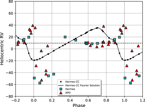
Figure 5. Hα Velocity Curve.
Download figure:
Standard image High-resolution imageIn Figure 6, we show the velocity curve for the Paschen lines, which are only minimally affected by departures from LTE because there are no metastable n = 3 levels. However, there may be small enhancements of the lower Paschen levels by collisional excitation of atoms in the metastable 2 s level. The 4 Paschen lines observed at Apache Point were 10 049.38, 8862.79, 8750.48, and 8598.39 Å. For the Hermes, spectra the line at 10 049 Å was outside the covered wavelength range. The 8750 Å line was sometimes not well defined due to blending by nearby features. Since there is some blending with stellar and atmospheric features, we show the velocity curves for each Paschen line with a different symbol. We also show the mean velocity of the four lines. The 10 049 Å line is the strongest and least blended but was observed only at APO. Its curve does not cover all phases, but it may be the most useful from just before minimum to just after maximum light, the phase at which Hα behaves most bizarrely.
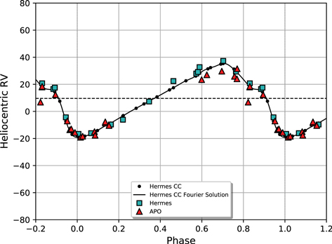
Figure 6. Hydrogen Paschen Velocity Curve.
Download figure:
Standard image High-resolution imageFor the higher Blamer lines (Hβ, Hγ, Hδ), blending distorts the line profiles so that it is difficult to assign a single velocity from a profile that is far from Gaussian in shape. For these lines, we have taken the mean velocity, which is shown in Figure 7.
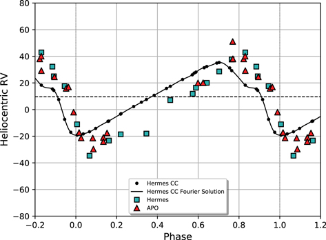
Figure 7. Average of Hβ, γ, δ Velocity Curve.
Download figure:
Standard image High-resolution image4.4. The O I Triplet
In Figure 8, we show the velocity curve for the O I triplet at 7771,4,5 Å. The O I curve extends from 32 km s−1 at minimum light to near –15 km s−1 near maximum light, which is very close to the amplitude of the CC curve. It is likely that the high excitation O I lines are formed over a wide region of optical depths. These three O I lines are unblended with other stellar features and are of moderate strength so that their wavelengths can be measured easily and accurately with the "k" command in the SPLOT routine of IRAF. Both curves show the inflection near 15 km s−1 on the descending velocity curve, which corresponds to the brief still-stand on the rising light curve.

Figure 8. O I Velocity Curve.
Download figure:
Standard image High-resolution image4.5. The Si II Pair at 6347.09 and 6371.36 Å
Because of the high excitation of 8.09 eV, these lines are formed deepest of any absorption lines in stars with the temperatures of Cepheids, with the possible exception of the Paschen lines, which are likely to be formed over a wide range of depth. Figure 9 shows the RV curve obtained from the Si II pair.

Figure 9. Si II Velocity Curve.
Download figure:
Standard image High-resolution image4.6. The Resonance Lines of Na I and K I
The zero-volt lines of these easily ionized elements are expected to be formed at small optical depths. Care has been used to distinguish the stellar components from possible blending with circumstellar and interstellar components as well as absorption by lines of the earth's atmosphere. Figures 10 and 11 show their velocity curves.
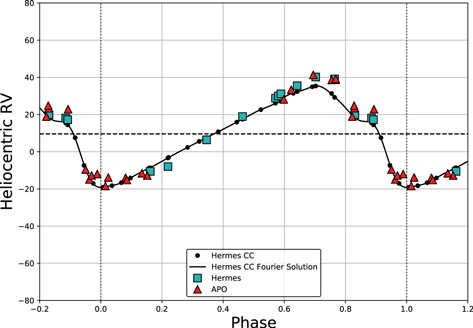
Figure 10. Na I Velocity Curve.
Download figure:
Standard image High-resolution image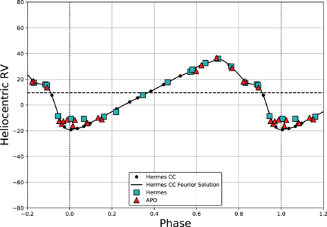
Figure 11. K I Velocity Curve.
Download figure:
Standard image High-resolution image4.7. The Ca II IR Triplet
The Ca II IR triplet is poised to gain in importance for Cepheid research thanks to the Gaia mission's RVS instrument that is observing timeseries radial velocities down to magnitude ∼15. Given the different velocities and amplitudes exhibited by different spectral lines, a comparison between the detailed spectral variability of the Ca II triplet and other, optical, spectral lines is particularly important.
Figure 12 shows the phase-resolved line profile variations as observed with Hermes for the 2015 and 2016 data.

Figure 12. Ca II IR triplet line profile variations as observed with Hermes for the 2015 and 2016 data. Phase sorting and colors are identical to Figure 4 and not labeled for clarity. Note the strong line splitting at phases close to minimum radius. The vertical dotted lines indicate minimum and maximum velocities listed in Table 1.
Download figure:
Standard image High-resolution imageThe Ca II IR triplet provides very valuable information because of its great strength and the fact that the majority of calcium atoms are singly ionized in Cepheid atmospheres. Such strong lines must be formed at small optical depths in the continuum. Profiles of the Ca II IR lines in a large number of non-pulsating stars have been presented by Linsky (1981). To understand the formation of the Ca II triplet lines, it is essential to take into account the lowest energy levels and transition probabilities of the Ca II atom. In Figure 13, we show an energy-level diagram for the lowest levels of Ca II. The triplet arises from the metastable 3D level that is sufficiently low that it is likely to be populated by collisions from the ground level. For a full discussion of the formulation of calcium absorption lines, see Osorio et al. (2019). A possible complication is the fact that atoms in the 3D and 4P levels may be ionized by Lyα photons (Wyse 1941). This sort of inter-species NLTE effect is very difficult to analyze quantitatively. In any case, the strong Ca II IR lines must be formed in the uppermost levels in the stellar atmosphere. The Doppler shifts and profiles exhibited by these lines are hence particularly sensitive to atmospheric dynamics and sensitive to model assumptions.
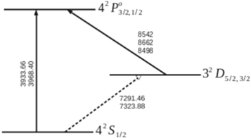
Figure 13. Energy-level Diagram for Ca II.
Download figure:
Standard image High-resolution imageThe Ca II triplet is particularly important because the great strength of all three lines gives them high weight in the radial velocity of F, G and K stars when measured by Gaia's radial velocity system. At most phases of X Cyg, the IR triplet lines appear to be symmetric and, hence, readily measurable for radial velocity. However, around light maximum they are asymmetric and, thus, show that two components are partially resolved at our resolution, indicating that two layers are simultaneously present in the stellar atmosphere. We show our measurements of the Ca II triplet lines in Figure 14. At maximum light, the Ca II IR curve lies well below the CC RV curve that represents the majority of the stellar atmosphere, and at minimum light, the Ca II IR curve lies significantly above the CC RV curve. Its behavior in Delta Cep is similar (Wallerstein et al. 2015). Further observations of a substantial number of Cepheids with a range in periods, as well as in other types of variables, are needed to understand and calibrate the use of the Gaia radial velocity system for pulsation research.
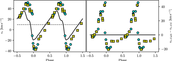
Figure 14. The Ca II IR triplet velocities compared to the Fourier series fit to the Hermes RV CC curve (solid black line). Yellow squares are based on Hermes spectra, Cyan circles on APO spectra. Note the much larger amplitude in the Ca II triplet and the phase shift relative to the RV CC curve at maximum and minimum. The right panel shows the difference between the two velocities. The Ca II minimum and maximum RVs occur with a phase shift of 0.067 (1.1 d) and 0.117 (1.92 d) after the RV CC reference.
Download figure:
Standard image High-resolution image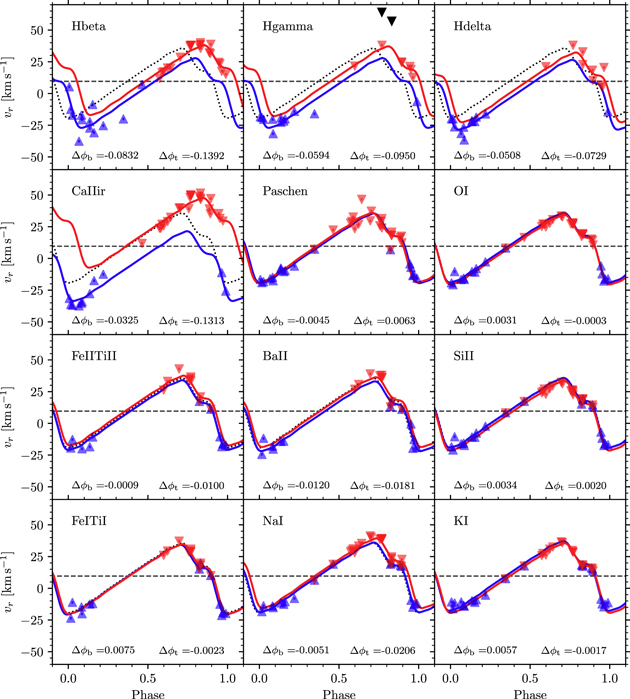
Figure 15. Phase offsets of individual line velocities relative to the Hermes CC RV curve determined by template fitting, cf. Table 3 and Anderson (2019) for a discussion of the method. The top and bottom parts of the individual line velocities were fitted separately using the CC RV template. Two apparently discrepant measurements for Hγ were ignored in the fit near maximum RV and are shown as black triangles.
Download figure:
Standard image High-resolution image
4.8. Emission at the H and K Lines of Ca II
Emission lines of Ca II in Cepheids were described by Herbig (1952) and more fully by Kraft (1956). During rising light and about coincident with the stand-still on the light curve, Ca II lines in emission appear due to gas moving outward at about 10 km s−1 faster than the gas that gives rise to the Ca II triplet in absorption. The IR triplet absorption lines then slowly rise, finally catching up with the CC curve at phase 0.6, which is nearly at minimum light near phase 0.7. The IR triplet lines reach a maximum velocity of 50 km s−1, about 0.1 cycle later than the CC curve, and by then represent matter falling in at 20 km s−1 faster than the CC curve. The IR lines continue to show an in-falling velocity relative to the CC curve, just about until maximum light after which they are replaced by the outward moving component. Just after maximum light, two spectra show a component near 45 km s−1, just as the CC curve reaches its minimum. This component appears at about the same time as the positively displaced components of Hα.
The H and K resonance lines of Ca II are very broad, strong, heavily blended and difficult to measure in such a way as to assign them a radial velocity. However, they show up in emission, probably formed in the chromosphere as is commonly seen in Cepheids and red giants (Kraft 1956).
5. Discussion
The primary purpose of this paper has been to assemble and display observed radial velocity data that will be of assistance in modeling the atmosphere of X Cyg as it goes through its pulsation cycle. Since all observed velocities are a weighted mean of true velocities over the surface of the star facing the observer, they must be converted to true motions of the gas by modifying the observed measurements by geometric and limb darkening effects. This is usually done by multiplying the observed velocity by a factor of 1.41 (Getting 1934). The calculation depends on the temperature gradient in the model stellar atmosphere which, in turn, may depend on the pulsation phase, since stellar atmospheres near maximum light are mostly radiative, but near minimum light are more likely to be substantially convective. Since most absorption lines are formed over a substantial optical depth, any velocity gradient within the layers in which the lines are formed will also influence the line profile. There is a recent discussion by Breitfelder et al. (2016) for various Cepheids with periods from 3.7 to 35 days. However, since RV amplitudes depend on the line species based on which they are measured, one may expect projection factors to depend on the (combination of) spectral lines used to measure the RVs. In particular, projection factors inferred from Gaia RVs that are measured on the Ca II NIR triplet may significantly differ from projection factors inferred from the currently widely-used optical cross-correlation velocities that are more similar to our Hermes observations.
In Figures 5 to 11, we display the observed velocity curves of X Cyg. In addition to the observed points, we show the mean curve as established from the high-resolution Hermes spectra by the cross-correlation method to represent the mean velocity of the atmosphere as a whole. The continuous line is the cross-correlation curve derived from the high-resolution Hermes data to represent the mean velocity of the atmosphere of X Cyg as a whole. Table 3 shows the results from fitting the CC radial velocity curve to the curves of the individual species. Figure 15 shows the phase offsets for individual line velocities.
In Figure 5, we show our measurements of the radial velocity of the Hα absorption line, whose unusual behavior was first noted by Kraft (1956), and illustrated by Greenstein (1960). Its behavior from minimum to maximum light was illustrated by Wallerstein (1983) from high-resolution photographic spectra and further reported by Butler & Bell (1997). The components seen in absorption in 1983 and 1997 are indeed present in the current data. The five points just before and at maximum light define gas that is falling into the star at 30–40 km s−1. The origin of this gas is not evident but we suspect that it is due to ionized gas that was ejected and is seen falling into the star after recombining, as seen in the solar chromosphere.
Between light maximum and phase 0.2, there are seven observations of Hα seen in both the Hermes and APO data, with a velocity between –40 and –60 km s−1. This new, rising gas, is perhaps the initiation of the next expansion. From phase 0.6 to 0.9 the velocity of Hα is constant and very close to the mean velocity of the star. Any effort to explain the observed velocities of Hα in absorption must take into account the meta-stability of the 2 s level from which the Balmer lines originate. The 2p level communicates with the ground level via Lyα, but Lyα photons must be strongly absorbed by interstellar gas in almost all Cepheids because of their distance.
The higher Balmer lines, Hβ, γ, and δ are shown in Figure 7. They tend to follow the metallic line absorption curve with a few positive discrepancies due to unrecognized blending or real discrepant behavior.
In Figure 6, we show the observed velocities of the Paschen lines. The Paschen lines define a smooth curve from about –20 km s−1 at maximum light to about 30 km s−1 near minimum light. The Paschen-δ line at 10 049 Å was measured only in the APO spectra. Their gross behavior follows the cross-correlation curve, but there are some differences depending on the source. Since the Paschen lines originate from the n = 3 level of H I, they are only minimally influenced by the overpopulation of the 2 s level from which the n = 3 levels may be populated collisionally.
The behavior of other species is less difficult to understand. In Figure 8, we show that the velocity curve of the O I triplet at 7771,4,5 Å, whose lower excitation is 9.1 eV, follows the basic velocity curve very closely despite the high excitation and well-known departure from LTE of these lines. The O I curve extends from about 32 km s−1 at minimum light to near –15 km s−1 at maximum light. The combination of the high concentration of O I and high excitation of the lower levels of the O I triplet, suggests that the O I lines are formed over a wide range in optical depth. This appears to be correct since the O I lines follow the cross-correlation curve very nearly. Also, shown in Figure 14 is the velocity curve of the Ca II IR triplet. For Ca II, the amplitude is quite a bit larger than the CC curve, ranging from about 40 km s−1 to –35 km s−1. It is likely that the strong Ca II lines represent levels significantly higher in the stellar atmosphere, however, only fully dynamical model atmospheres can test these suggestions.
The two lines of Si II at 6347 and 6371 Å shown in Figure 9 arise from 8.09 eV and, because these lines are formed at high excitation levels that require 8.11 eV to be ionized from Si I, they are primarily formed at large optical depths in solar-type and cooler stars (Frazier 1966). They follow the Hermes velocity curve rather closely, except that they turn down at maximum velocity a little earlier than does the Hermes curve as was noted in the 1983 data. The curve for Na I in Figure 10 follows the Hermes curve fairly well except that at maximum velocity, it turns down later than the Hermes curve. This is due to the low ionization potential of Na I, which results from the Na I lines being formed higher in the Cepheid atmosphere. For K I, shown in Figure 11, the early turn down is not evident probably due to the low abundance of K as compared to Na causing the K I resonance lines to be formed over a greater interval in depth than the Na I lines. Table 4 shows the velocity amplitude, i.e. maximum-minimum velocity, for each of the species tracked in this paper. The amplitude of the Ca II IR triplet lines are the largest by far.
6. Summary
We have derived velocity curves of the 16-day classical Cepheid X Cyg from echelle spectra with a resolution of 30 000 and 85 000. The overall behavior of the star is shown by the cross-correlation method and individual velocity curves for Balmer, Paschen, O I, Si II, Na I and K I to illustrate the depth dependence of the velocity changes during the pulsation cycle. By including wavelengths out to 10 050 Å, the Paschen lines and the Ca II IR triplet are included for the first time for a long-period Cepheid. The Ca II triplet is particularly interesting because it is included in the Gaia high-resolution velocity band and probably dominates the Gaia velocities for F, G, and K stars.
We thank the observers who have contributed to gathering the Hermes spectra.
This research is based on observations made with the Mercator Telescope, operated on the island of La Palma by the Flemish Community, at the Spanish Observatorio del Roque de los Muchachos of the Instituto de Astrofísica de Canarias. Hermes supported by the Fund for Scientific Research of Flanders (FWO), Belgium, the Research Council of K.U. Leuven, Belgium, the Fonds National de la Recherche Scientifique (F.R.S.-FNRS), Belgium, the Royal Observatory of Belgium, the Observatoire de Genève, Switzerland, and the Thüringer Landessternwarte, Tautenburg, Germany.
Facility: Mercator1.2m. -
This research is also based on observations obtained with the Apache Point Observatory 3.5-meter telescope, which is owned and operated by the Astrophysical Research Consortium.
Facility: ARC3.5m. -
The AAVSOnet and its Epoch Photometry Database were made possible through the generous contributions of James Bedient, Donn Starkey, Doug Welch, Tom Krajci, Peter Nelson, Bill Stein, Greg Bolt, Bob Stine, Mike Linnolt, Richard Berry, David Benn, John Gross, Doug George (Cyanogen), Bob Denny (DC3 Dreams), and the Santa Barbara Instrument Group (SBIG).
B. Lacy's current affiliation is 4 Ivy Lane, Princeton University, Princeton NJ 08544.
Footnotes
- 7
As discussed in Paper I, the Fourier representation is a mathematical analogy compared with a physical analogy as represented by a pulsating model atmosphere.