Abstract
The Gaia mission will provide a six-parameter solution for millions of stars, including a tridimensional map of our Galaxy. The estimation of distances has been made for the Tycho-Gaia Astrometric Solution (TGAS), while to contrast the proper motions it is interesting to consider positions from the different Gaia Data Release with older ones given in ground-based massive catalogs. This process has been followed to build, for example, the PMA catalog using the 2MASS. Our aim is to improve the positions of this catalog (although the process is applicable to any other). The first stage, presented here, consists of carrying out a three-dimensional study using vector spherical harmonics (VSH) development of the systematisms in position for the stars common with Hipparcos-2; we take into account the distances, magnitudes, and spectral types. To this aim, we use linear polynomial regression of first order that fits vector fields and the derivatives of their components. We verify that the coefficients of the developments of first order have different behavior according to the characteristics of stars and distances. To deepen the study, we focus on the conservative component of the field, applying the Helmholtz theorem. Each potential function is obtained solving a Poisson equation on the sphere, after finding the divergence of the corresponding vector field. Both vector and potential fields present patterns, at certain points, that depend on the three considered parameters (distance, magnitude, and spectral type); their sources and shrinks correspond to maxima and minima. In this sense, we observe that these critical points are also critical points of the surface that represents the VT magnitude of Tycho-2, which makes sense because this catalog was used in the reduction of 2MASS positions. Finally, we selected some stars near the critical points of the vector fields and apply the adjustments obtained in the previous sections. The difference with the positions in DR1 allows us to compare the proper motions: those from the PMA and those induced after our corrections.
Export citation and abstract BibTeX RIS
1. Introduction
Astrometry is an astronomical discipline whose objective is to determine positions, parallaxes, and proper motions in the most accurate way possible. In the last decades, since Hipparcos mission (that provided Hipparcos and Tycho catalogs Perryman & ESA 1997), a much more precise determination for astrometric parameters, in particular for parallaxes, was possible than the one obtained using observations from Earth. The uncertainties, taking as reference the improved version—Hipparcos-2 henceforth—by van Leeuwen (2007a, 2007b) are 0.3 mas for positions and parallaxes and 1 mas/yr for proper motions (data valid for J1991.25). The approximately 120,000 stars contained in the catalog are, at best, an order up to 11.5 of H-magnitude. The Hipparcos catalog is the realization of the Hipparcos Celestial Reference Frame (HCRF), which was aligned with the International Celestial Reference Frame (ICRF) with the aim of having no system rotation. The estimated error on the expected accuracy of the system rotation of the HCRF with respect to the ICRF was 0.25 mas/yr.
In the framework of the Gaia mission (Prusti et al. 2016), the Gaia satellite was launched in 2013 with the objective (see Arenou et al. 2017) of "measuring the three-dimensional distribution, both in position and in speed, of the stars of our galaxy, as well as the determination of their astrophysical properties." The astrometrical content of Gaia Data Release 1, (DR1; Lindegren et al. 2016), consists of two parts: the primary and the secondary data sets. The first contains positions, parallaxes, and proper motions for the stars common with the Tycho-2 catalog (Høg et al. 2000), obtained by means of the so-called Tycho-Gaia Astrometric Solution (TGAS) solution (Michalik et al. 2015). For more details in the precedents of the TGAS construction, see the Agis paper (providing an Astrometric Global Iterative Solution (Lindegren et al. 2012) and their application by Michalik et al. (2014) to obtain the HTPM solution (without using Tycho's stars). For estimated accuracy of TGAS regarding the 96365 stars common with Hipparcos, the J1991.25 positions have been taken as valid, while the proper motions are estimated to have an accuracy of 0.06 mas/yr and the parallax 0.3 mas (plus another 0.3 mas for a systematic component; see Brown et al. 2016). It is very reasonable to expect that these precisions will improve after the final stage of the 5 year mission (despite having published DR2 in April 2018 (Brown et al. 2018), and other papers included in this special issue, which have not been considered in this paper). This DR1 parallax system is independent of the Hipparcos parallax system, but the comparison carried out by Lindegren et al. (2016) concludes that the accuracies in both systems are comparable for the Hipparcos stars. Since the publication of DR1, different studies have been carried out on systematic errors, mainly in parallaxes. For instance, Stassun & Torres (2016), using 158 eclipsing binary stars and finding some correlations with the ecliptic latitude, but not with brightness or color (Zinn et al. 2017; Gontcharov 2017; Davies et al. 2017; Ridder et al. 2016; Schönrich & Aumer 2017). Also, regarding the proper motions, the PMA catalog (Akhmetov et al. 2017) has been built from the data of DR1, UCAC5 (Zacharias et al. 2017) and a modification of the 2MASS (Cutri et al. 2003; Skrutskie et al. 2006). These papers, among others, make us think that it may be of interest to consider the use of massive catalogs (although this mass property it is not necessary: the use of the complete catalog or a subset may be possible, considering the characteristics of our study) to track the consistency/inconsistency in certain parameters measured from different catalogs. In this paper, we have the two-fold purpose of studying the global and local aspects of the residual three-dimensional vector fields obtained by different comparisons between two astromeric catalogs. More specifically, from the residuals in right ascension and declination, we will consider the discrete three-dimensional vector field associated with these data, with the goal of identifying possible systematic differences depending on a set of parameters like magnitudes and spectral types for each fixed distance. On the one hand, we consider Hipparcos-2 (van Leeuwen 2007a) with the values of the distances of TGAS, as estimated after the studies of Bailer-Jones (2015) and Astraatmadja & Bailer-Jones (2016a, 2016b). In this sense, it is interesting to note that the measurement of a parallax is a "noisy measure" of the inverse of the distance. Thus, it is only possible to assign a probability to the distance using Bayes Theorem, from parallax observations and an a piori distribution of distances in the Galaxy. It is precisely in this last article where the catalog of distances for the TGAS catalog is attached. Its existence enables us to carry out a study, with a good precision, in the interval [25; 600] pc, taking slices centered at r = 100, 200, 300, 400, and 500 pc in equatorial coordinates, without having to use the inverse of the trigonometrical parallaxes of Hipparcos. A brief comment about this will be made in Section 2.1. On the other hand, we have chosen as second catalog the 2MASS catalog for two reasons: first, because of its use in PPMX (Röser et al. 2008) and the PPMXL (Röser et al. 2010) position systems and also, because the UCAC4 (Zacharias et al. 2013) astrometric reduction was made applying certain corrections in which the 2MASS catalog was used to refer to Tycho-2; and second, for being a completely independent catalog from Hipparcos, although the stars of Tycho-2 were used to obtain the reductions. Comparison of the 2MASS point-source positions with the Tycho-2 catalog shows that 2MASS positions are consistent with the ICRS with a net or a set no larger than 15 mas. Similar uncertainty, at best, is achieved for the UCAC4 stars. Some studies about the differences using 2MASS and the UCAC catalogs can be seen in Zacharias et al. (2000, 2004) and Zacharias et al. (2013).
Regarding the methods used for the comparison of catalogs, it is particularly noteworthy that they have been evolving in the last decades because a greater precision in the measurements demands a greater refinement in the theoretical adjustment models. Thus, in the mid 1960s, the spherical harmonics were already used in the field of physical geodesy (Heiskanen & Moritz 1967). At about same time, Brosche (1966) used them for the first time to calculate the systematic part of the residuals obtained by comparing different stellar catalogs (English version in 1966). This approach allowed the independent development of residuals in R.A. and decl. A joint treatment for R.A. and decl. required the use of vector fields over the sphere and its development, under the hypothesis of regularity (the completeness theorem can be found in Jeffreys 1967), in vectorial spherical harmonics (VSH henceforth). This method was introduced by Mignard & Morando (1990) in the field aimed at this paper, while an early introduction about the general principles of VSH can be found in the classic work of Morse & Feshback (1953). This method, applied to the vector fields of residuals both in the projection on the celestial sphere and in different slices, is the one that we apply here. In addition, to see how the spectral types and magnitudes affect the results, classifications have been made: (a) KM/(Non-KM); (b) magnitudes in m4/m5/m6/m7 sets (defined in the article); and (c) subsets obtained mixing the two previous pure types (KM-m4 to KM-m7 and the same for No-KM). All of these methods have been studied over the whole sphere and with the spatial subdivision by slices; then, the three-dimensional study has been performed, so that the results can be compared in both cases. This part of our work concerns the global part of the study. We must mention that the treatment of the data will be carried out through a suitable regression method. More specifically, we use local polynomial regression of first order, fitting the components of the vector fields and the derivatives of these components (it is important to know that we compute estimators for functions and their derivatives, not for the derivatives of the estimator functions). These technical topics will be presented in Section 3, after a study of the data in their quantitative (Section 2.2) and qualitative aspects (Section 2.3). Regarding the analysis of the vector field of the residuals, we know that the toroidal harmonics correspond to the rotational part of the field, and its calculation up to order one can be sufficiently representative. However, this does not happen with the non-rotational part of the vector field. To obtain a more accurate study, we have considered the Helmholtz theorem, which splits each vector field into two components: rotational and non-rotational. This second part coincides with the gradient of a potential function (so the divergence of the residual field coincides with the Laplacian of such a potential function; see Section 4). Thus, it is possible to obtain a high-order development of the potential function in each slice. To calculate both expressions, we use local first-order polynomial estimators in three dimensions, providing adjustment for the function and its derivatives to calculate the divergence of the vector field. For the second member of the equation, we apply the properties of spherical surface harmonics as eigenfunctions of the Laplace-Beltrami operator. The areas of the sphere, for each slice, in which the critical points of the global field and the critical points of the potential are close and of no interest from the rotational point of view; however, they are of interest from the non-rotational point of view. This is the local part of the work. Once the critical points of the residual vector field for each slice have been related to the critical points of a certain potential function, we have considered the possibility of finding a physical quantity that is relevant in the reduction of data and that may be related to these critical points of the potentials found. In this sense, given that Tycho-2 was the reference chosen in the reduction of positions of the 2MASS stars, we have studied the surfaces determined by the BT and VT magnitudes. It has been checked that in the neighborhood of the critical points of the vector fields, the same type of critical point appears on the VT surface (sometimes the BT also behaves the same, but less clearly than the VT; this is probably due to, or is related to, the fact that this magnitude is closer to the absolute magnitude, but this is merely a speculation) It is interesting to remark that the sources and shrinks (also the saddle points) are patterns that appear depending on the stellar classification carried out (but not necessary in the residual vector field on the whole sphere), while the relative extrema of the surfaces of VT magnitude, appear when we consider all the stars from Tycho-2 in the neighborhood of each point as, obviously, in the process of reduction of the 2MASS did not directly influence the stellar distances. Results are presented in Section 5. We summarize our conclusions in Section 6.
To visualize other possible applications, once the work has been carried out with all the data of the 2MASS in the sense explained above, we have computed some proper motions induced by the corrections obtained in Section 5.1 in the neighborhood of some of the singular points of the vector fields presented in 5.2. We proceed to compare the obtained results with those of DR1 and those of the PMA, which, as mentioned, reviewed 2MASS prior to the calculation of its proper motions.
2. Previous Studies of the Data
2.1. A Brief Note about the Use of Distances
Regarding the use of the inverse of the parallax as distance, there are numerous papers in which such equality is used for distances near the Sun (for example, we can highlight Vityazev & Tsevtkov 2009; Vityazev et al. 2011; Makarov & Murphy 2007), which applies to a subset of 42,487 stars of Hipparcos fulfilling that π/σ(π) > 5 or Vityazev et al. (2017c)). On the other hand, in the 1997 version of Hipparcos, the uncertainties in the parallaxes were 1 mas, so Lutz-Kelker bias was not considered before 200 pc. However, given that there are new estimates for the stars of Hipparcos-2 from the publication of TGAS distances introduced in Astraatmadja & Bailer-Jones (2016a) and the corresponding data catalog at http://www.mpia.de/homes/calj/tgas_distances/main.html, we have decided to make use of these new data.
However, in a preliminary study related to the use of the inverse of the trigonometric parallax as a biased approximation of the distance, we have created 1000 samples from the initial data, perturbing the R.A. and the decl. by a N(0, 1) and the inverse of the parallax by 20% of its value times a N(0, 1) We have verified that, considering all the samples, if we call mi and Mi the minimum and maximum values, for the i-star, of the "distances" in Hipparcos-2 with the application of the disturbance, 90% of the stars that we have used verifies that ri < dGi < Mi, where dGi are the distances provided in the file appended to Astraatmadja & Bailer-Jones (2016a), which could show a relatively high reliability in the results that will be obtained in our studies, in 3D, of the residuals for the stars of Hipparcos-2 compared with the corresponding positions in another catalog. In spite of this, given the aforementioned availability of distances for the stars of the TGAS, we have used them although the positions and proper motions are those corresponding to Hipparcos-2. With this choice, the reliability of our method and later results are based on a disturbance test with lower requirements, in which the R.A. and the decl. are still added a N (0, 1), but to the distance, a 10% of itself times a N(0, 1) is added. Before that, in the following two subsections, we show the results of some elementary statistical studies about the qualitative and quantitative aspects of the data considered.
2.2. Data Quantitative Aspects
We initially consider the 66,577 stars common to Hipparcos 2 (van Leeuwen 2007b) and 2MASS (Skrutskie et al. 2006) with known TGAS distances; we eliminate double stars, those with negative parallax, considering that both residuals Δα*, Δδ are, in absolute value, minor than 200 mas. Under these conditions, we have the initial statistics seen in Table 1 (Dr indicates the domain to which the data in the corresponding line refer). We consider overlapping for a better follow-up of the continuity or discontinuity of the different quantities.
Table 1. Initial Statistics for 2MASS-Hip2 for Stars between 25 and 600 pc
| Centered at r = | Dr | N |

|

|

|

|

|

|
|---|---|---|---|---|---|---|---|---|
| S2 | 58081 | 345.58 | 0.66 | 5.82 | 0.21 | 4.34 | 117.55 | |
| 100 |
![${\left[25,200\right]}^{}$](https://content.cld.iop.org/journals/1538-3873/131/998/044501/revision1/paspaaed5dieqn7.gif)
|
24498 | 125.34 | 1.37 | 8.41 | 1.08 | 7.55 | 124.19 |
| 200 |
![$\left[100,300\right]$](https://content.cld.iop.org/journals/1538-3873/131/998/044501/revision1/paspaaed5dieqn8.gif)
|
30455 | 192.93 | 0.43 | 6.29 | 0.33 | 6.29 | 118.58 |
| 300 |
![$\left[200,400\right]$](https://content.cld.iop.org/journals/1538-3873/131/998/044501/revision1/paspaaed5dieqn9.gif)
|
23219 | 288.88 | −0.09 | 5.34 | −0.11 | 5.39 | 114.71 |
| 400 |
![$\left[300,500\right]$](https://content.cld.iop.org/journals/1538-3873/131/998/044501/revision1/paspaaed5dieqn10.gif)
|
16224 | 386.69 | 0.40 | 4.17 | 0.48 | 4.03 | 113.32 |
| 500 |
![$\left[400,600\right]$](https://content.cld.iop.org/journals/1538-3873/131/998/044501/revision1/paspaaed5dieqn11.gif)
|
10364 | 482.60 | 1.15 | 2.80 | 1.10 | 2.84 | 112.50 |
Download table as: ASCIITypeset image
We calculated the mean of  for each slice, and the means in Δα*, Δδ in two different ways: the usual arithmetic mean and the weighted mean with the distance in pc:
  . Finally, the square root of the power
 ![$\sqrt{\tfrac{{\left[{\rm{\Delta }}{\alpha }_{i}^{* }\right]}^{2}+{\left[{\rm{\Delta }}{\delta }_{i}\right]}^{2}}{N}}$](https://content.cld.iop.org/journals/1538-3873/131/998/044501/revision1/paspaaed5dieqn14.gif) is provided.
is provided.
We can observe that the means in Δα*, Δδ are very similar, no matter if the weighting is the classical arithmetic or the one given by the distances. This may imply that the dependence Δα*(r), Δδ(r) is very accurate for the TGAS distances. The graphs of the density functions in Δα*, Δδ, and r can be seen in Figures 1 and 2. The indication of the dependence of Δα*(r) and Δδ(r) can be seen in Figure 3.
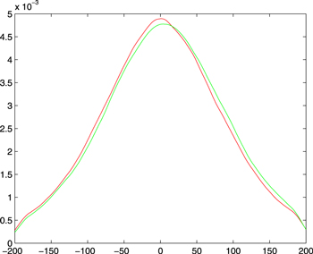
Figure 1. Density functions for  (red) and
  (green), in mas.
Download figure:
Standard image High-resolution image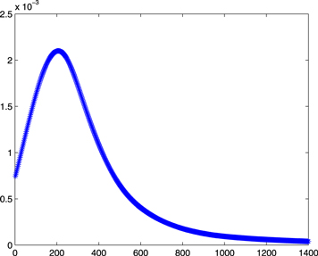
Figure 2. Distribution of r (in pc) for 2MASS.
Download figure:
Standard image High-resolution image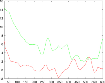
Figure 3. Graphic in smoothed means of  (red) and
  (green), in mas.
Download figure:
Standard image High-resolution imageAnother aspect to consider is the lack of normality of Δα*, Δδ (see, again, Figure 1 for the 2MASS). This rather points to a "Gaussian mixture" which confirms our interest to study different subsets of data, with respect to magnitudes or spectral types, for example. The dependence of r, and also some physical properties, would indicate the search for clusters from a statistical point of view (not to be confused with star clusters). Finally, the distribution in r indicates that a large percentage of our star set has a radius  , so we have selected the stars up to such a distance because our aim is devoted to the slices centered at the distances r = 100, 200, 300, 400, and 500 pc. Employing these restrictions, only 58,081 stars remain.
2.3. Data: Qualitative Aspects
The magnitude is a property whose influence has been studied by Bien et al. (1978) and Schwann (2001) among others. In this section, we only give a brief description of the data which , in our case, take values between Hp-magnitudes −1.088 and 14.169. Figure 4 gives an idea of their probability density function (Hmag is taken from the Hipparcos2 catalog, and is represented here as Hp).

Figure 4. Density function for Hp-magnitude.
Download figure:
Standard image High-resolution imageArtificially we have made a subdivision into  subintervals and have subsequently classified the stars according to
  slices of
  . Approximately 75% of the stars are concentrated in the subsets that we have called m5 and m6, but other magnitudes have also been considered that also have good representativity in some of the selected
  intervals. More specifically, if m4 = [5.750, 7.153], m5 = [7.153, 8.556], m6 = [8.556, 9.959], m7 = [9.959, 11.363] and we consider the distances
 ![$\left[25,600\right]$](https://content.cld.iop.org/journals/1538-3873/131/998/044501/revision1/paspaaed5dieqn24.gif) pc. The numerical distribution can be seen in Table 2.
pc. The numerical distribution can be seen in Table 2.
Table 2.
Numerical Distribution Regarding r and Number of Stars of the  2MASS Subsets
| Centered at r = | Dr | m4 | m5 | m6 | m7 |
|---|---|---|---|---|---|
| S2 | 4707 | 24888 | 28103 | 4263 | |
| 100 |
![${\left[25,200\right]}^{* }$](https://content.cld.iop.org/journals/1538-3873/131/998/044501/revision1/paspaaed5dieqn26.gif)
|
2947 | 9742 | 9968 | 1632 |
| 200 |
![$\left[100,300\right]$](https://content.cld.iop.org/journals/1538-3873/131/998/044501/revision1/paspaaed5dieqn27.gif)
|
2844 | 13048 | 12215 | 2254 |
| 300 |
![$\left[200,400\right]$](https://content.cld.iop.org/journals/1538-3873/131/998/044501/revision1/paspaaed5dieqn28.gif)
|
1331 | 10248 | 9867 | 1712 |
| 400 |
![$\left[300,500\right]$](https://content.cld.iop.org/journals/1538-3873/131/998/044501/revision1/paspaaed5dieqn29.gif)
|
624 | 6031 | 8558 | 952 |
| 500 |
![$\left[400,600\right]$](https://content.cld.iop.org/journals/1538-3873/131/998/044501/revision1/paspaaed5dieqn30.gif)
|
309 | 3588 | 5866 | 568 |
Download table as: ASCIITypeset image
With respect to the spectral type, we have differentiated the two KM groups (K or M type) and the rest, obtaining 17243 for the first and 40838 for the second group, always with the general conditions indicated in the preceding subsection. Global distributions for KM and No-KM stars can be seen in Figure 5 and their statistics in Table 3, where we can see some information about the bias in the distributions of stars in KM and No − KM. Namely, the former subset has a greater bias in Δα*, while the latter subset has a greater bias in Δδ. In Table 4 we show the statistics for the spectral type in each of the magnitude subgroups.
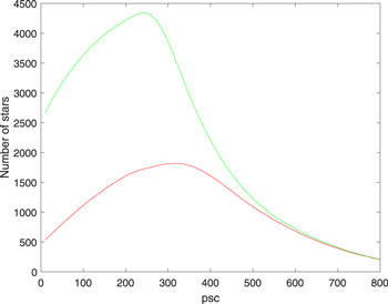
Figure 5. Star distribution for type K or M (KM) stars (red) and the rest (No-KM) (green).
Download figure:
Standard image High-resolution imageTable 3. Numerical Distribution (in mas) of Stars of Spectral Type from K to M and the Rest. Stars from 25 pc to 99 pc are Included, and also Subdivision by Intervals Centered at r from 100 pc to 800 pc. 2MASS-Hip2. r is the Value in pc Where the Slice is Centered
| Spectral | r = | Dr | N |

|

|

|

|

|

|

|
|---|---|---|---|---|---|---|---|---|---|---|
| S2 | 40838 | −0.73 | 7.26 | 82.32 | 80.88 | −1.78 | 5.91 | 115.6 | ||
| No KM | 100 |
![$\left[25,200\right]$](https://content.cld.iop.org/journals/1538-3873/131/998/044501/revision1/paspaaed5dieqn38.gif)
|
21360 | 0.50 | 8.66 | 88.29 | 84.52 | 0.21 | 7.97 | 122.6 |
| 200 |
![$\left[100,300\right]$](https://content.cld.iop.org/journals/1538-3873/131/998/044501/revision1/paspaaed5dieqn39.gif)
|
24286 | −0.41 | 6.87 | 83.24 | 81.25 | −0.54 | 6.65 | 116.5 | |
| 300 |
![$\left[200,400\right]$](https://content.cld.iop.org/journals/1538-3873/131/998/044501/revision1/paspaaed5dieqn40.gif)
|
14740 | −1.17 | 5.81 | 77.56 | 78.01 | −1.25 | 5.85 | 110.2 | |
| 400 |
![$\left[300,500\right]$](https://content.cld.iop.org/journals/1538-3873/131/998/044501/revision1/paspaaed5dieqn41.gif)
|
8465 | −2.03 | 5.09 | 75.18 | 76.24 | −2.08 | 4.50 | 107.2 | |
| 500 |
![$\left[400,600\right]$](https://content.cld.iop.org/journals/1538-3873/131/998/044501/revision1/paspaaed5dieqn42.gif)
|
4738 | −3.38 | 4.94 | 72.84 | 75.17 | −3.52 | 5.01 | 104.8 | |
| S2 | 17243 | 4.01 | 3.45 | 86.62 | 87.15 | 4.03 | 1.87 | 123.0 | ||
| KM | 100 |
![$\left[25,200\right]$](https://content.cld.iop.org/journals/1538-3873/131/998/044501/revision1/paspaaed5dieqn43.gif)
|
3138 | 7.31 | 6.65 | 97.68 | 92.57 | 7.18 | 4.56 | 134.9 |
| 200 |
![$\left[100,300\right]$](https://content.cld.iop.org/journals/1538-3873/131/998/044501/revision1/paspaaed5dieqn44.gif)
|
6169 | 3.77 | 3.99 | 89.94 | 88.71 | 3.21 | 3.98 | 126.4 | |
| 300 |
![$\left[200,400\right]$](https://content.cld.iop.org/journals/1538-3873/131/998/044501/revision1/paspaaed5dieqn45.gif)
|
8479 | 1.79 | 4.53 | 86.03 | 86.65 | 1.73 | 4.65 | 122.2 | |
| 400 |
![$\left[300,500\right]$](https://content.cld.iop.org/journals/1538-3873/131/998/044501/revision1/paspaaed5dieqn46.gif)
|
7759 | 3.06 | 3.15 | 83.64 | 85.41 | 3.21 | 3.00 | 119.6 | |
| 500 |
![$\left[400,600\right]$](https://content.cld.iop.org/journals/1538-3873/131/998/044501/revision1/paspaaed5dieqn47.gif)
|
5626 | 4.96 | 1.0 | 82.27 | 85.24 | 4.94 | 1.05 | 118.6 | |
Download table as: ASCIITypeset image
Table 4. Numerical Distribution (in mas) of 2MASS-Hip2 Stars of Spectral Type from K to M and the Rest. Subdivision by Magnitudes are Included, Considering only our m4, m5, m6, and m7 Subsets
| Spec/Mag | N |

|

|

|

|

|

|
|---|---|---|---|---|---|---|---|
| No KM | |||||||
| & m4 | 3185 | −1.55 | 4.61 | 86.11 | 86.45 | −4.00 | 4.69 |
| & m5 | 15392 | −0.72 | 6.50 | 83.96 | 83.50 | −3.24 | 4.80 |
| & m6 | 18765 | −0.64 | 6.62 | 80.77 | 79.47 | −2.06 | 5.65 |
| & m7 | 3329 | −3.74 | 13.90 | 73.26 | 66.89 | −4.58 | 11.07 |
| KM | |||||||
| & m4 | 1402 | 15.95 | 2.20 | 95.91 | 96.39 | 19.34 | 4.75 |
| & m5 | 8186 | 4.80 | 2.94 | 88.38 | 90.17 | 7.40 | 1.69 |
| & m6 | 6936 | 2.46 | 3.48 | 81.71 | 82.54 | 2.56 | 2.28 |
| & m7 | 583 | −4.33 | 6.63 | 90.22 | 87.09 | −2.74 | −0.81 |
Download table as: ASCIITypeset image
3. Methods
In this section, we present a brief justification of why we use other than the current procedures to deal with the problem. Next, we will introduce the formulations that allow to deal with the problem from a continuous point of view.
3.1. Continuous versus Discrete Problem
The problem with the three-dimensional study of the differences has recently been partially addressed by Vityazev & Tsvetkov (2013) to the residuals of Hipparcos2 and UCAC4. Such work has taken into account the discrete set of data, the adjustment model, and the statistical method for the allocation of formal errors and, if appropriate, the acceptance or denial of a determined computed value for some parameter (contrast of hypotheses).
However, it is possible to go back to the work of Mignard & Morando (1990) to see the use of VSH in catalog problems. From then, two issues regarding catalogs have been studied, the one concerning the position and that of the kinematical study of the galaxy from the proper motions. About the former, we can highlight its application to Hipparcos-FK5 (Mignard & Klioner 2012) and (Marco et al. 2004), or to those made by Vityazev et al. for the UCAC4-PPMXL (Vityazev & Tsevtkov 2015), XPM-UCAC4 (Vityazev et al. 2017a), among others. Regarding the application in kinematic studies, we can mention those obtained by Vityazev & Tsevtkov (2009) with Hipparcos and a catalog test between 200 and 300pc, Vityazev et al. (2011) for Tycho-2; Vityazev & Tsvetkov (2013) for UCAC4; Vityazev & Tsevtkov (2014) for UCAC4, PPMXL, and XPM; Vityazev & Tsvetkov (2017b) for Tycho-2 using TGAS; and Vityazev et al. (2017c) for UCAC4, PPMXL, TGAS, using RAVE5; and the use of VSH in Marco et al. (2015) applied to the proper motions of Hipparcos2 and introducing nonparametric methods of adjustment. We can also reference the study conducted by Mignard (2000), which, although it does not use VSH, does make an interesting distinction between spectral types for the results of OMM model of the Hipparcos kinematics.
As we have already mentioned in previous articles (Marco et al. 2004, 2015), the choice of model requires assuming that the function to be adjusted belongs to a certain space of functions and then the least-squares integral condition is applied, which allows the calculation of the parameters. The fact of working with a discrete set of data makes such calculations to actually be estimates. In this sense, most authors prefer to make discrete least-squares adjustments (which we will call DLS). Accepting, of course, that this procedure provides the coefficients for the least-variance unbiased estimator (in the discrete sense), there are some facts that make us think of a variation of the procedure. First, the original data are not necessarily unbiased (this is why the estimator obtained—the model with the corresponding coefficients—will not be the unbiased minimum variance estimator). Second, remember that the data are being adjusted to a continuous function and the model is nothing more than the truncated development, up to the desired order, of an infinite series. Such series development can be assumed to exist for a function with square integrable in the working domain (for example, in the sphere). The fact of working with the DLS method implies that no use is made of the analytical properties in which the continuous problem is formulated, and a good part of the power of the theoretical procedure may be lost. We then go on to describe the continuous extent of the problem.
Suppose that we want to determine a function f(x) belonging to a Hilbert space H, with  , the work domain, and that function verifies the necessary hypotheses that assure the existence of a convergent series development (not punctual convergence, but convergence in the norm of the functional space). Suppose we work with an orthogonal basis,
  . Then, the completeness property tells us that there exist (unique) coefficients
  such that

Remember that this equality is, in fact, symbolic. What it really means is that

where  represents the norm associated to the inner product in H denoted by
  . Thanks to the orthogonality and completeness properties of the basis, we can assure that

The importance of this formula is that each coefficient is found independently of the others. Note that this does not happen with a discrete treatment of the problem because in this case, we have to choose an a priori order for the development, and if we decide to increase that order, the coefficients must be recalculated again. This is a huge drawback. The reason is that the functional orthogonality of the basis enables the previous formula to be exact for each index. In the discrete case, with the DLS method, the theoretical functional orthogonality does not become algebraic orthogonality of the normal matrix that estimates the coefficients. This is why recalculation is mandatory if the order of development is changed. On the contrary, a discrete formulation in which we select a mesh in the domain D with equispaced points (in each dimension of D), retains the theoretical functional orthogonality to that discrete step. Then, you would get approximate values

where  are approximations obtained by working in the discrete space Hm, m representing the discrete meshing and
  the discretization of the inner product in H. No recomputation of the coefficients is required if the order is increased.
In our case, the Hilbert space will be that of functions (or vector fields) of square integrable in the sphere:  , and the v product will be the integral over the sphere. Note that the calculation of the estimates of
  will be performed by applying a numerical integration. To complete the procedure, we only need to see how to determine
  . Recall that we initially started from a set of discrete data,
  , and we can assume that they are realizations of random discrete or continuous variables. We work on the second assumption, and we will use nonparametric kernel estimation and kernel local polynomial linear regression that is useful for working with vector fields.
3.2. Kernel Estimations
In this subsection, we provide the exposition of the procedures for determining density functions, unidimensional regressions to fit the function, and multidimensional local polynomial formulation (which adjusts the function and the partial derivatives up to a predetermined order, which for us will be only one). During the brief presentation, the necessary references will be cited for an extension of the concepts, including theoretical results as well as their practical application.
3.2(a). A kernel K is a non-negative function, defined in a domain D, such that  ,
,  , and
, and  . Simple and usual examples are the Epanechnikov kernel,
  , or the Gauss kernel,
  . Its properties, in terms of statistical efficiency, can be found in Simonoff (1996), Fan & Gijbels (1996), or Wand & Jones (1995). The density function f(x) of a random variable (r.v.) X is estimated by

where  are the discrete data of the r.v., and hx is the so-called bandwidth which can be constant or variable and in which the subindex refers to the r.v. The higher the value of hx, the smoother the estimator; the lesser the value of hx, the lesser the smooth estimator. The optimization of this parameter is done by minimizing the asymptotic mean integral squared estimation (AMISE), whose value for this one-dimensional problem is
  , with N the size of the sample, and
  the standard deviation of the data. This topic and the extension to the multidimensional case is immediate, and can be seen in the previous references. The optimal values of the bandwidth are obtained in the case of a dimension, d, as
  (Simonoff 1996), with H the vector of the different values of h and Σ the variance–covariance matrix.
3.2(b). Let us now consider the case of an r.v. (X, Y) with discrete data  . Let
. Let  denote the kernel estimate of the joint density function. If we assume that the r.v. Y depends on the r.v. X, the regression of Y on X will be
  . The precise definition is
 ![$y=m(x)=E\left[\left.Y\right|X=x\right]\,=\int {{yf}}_{\left.Y,| \right|X=x}(\left.y\right|X=x){dy}$](https://content.cld.iop.org/journals/1538-3873/131/998/044501/revision1/paspaaed5dieqn77.gif) , where
, where  is the conditional probability which, by the total probability theorem, verifies that
  (hereafter, we will omit references in densities to r.v.s, except where the context requires otherwise). A substitution in the exact formula of the regression, but applying the kernel approximations of the densities (since they are unknown), provides an estimate of the regression, known as Nadaraya-Watson (to avoid the danger of confusion, we use h instead of hx):
It is interesting to remark that the Nadaraya-Watson method has the following characteristic: if Y is an r.v. dependent on another r.v. X, the estimation at a point x is the value  that minimizes (in β) the expression

which is nothing more than the discretization (from integral to summation) of the variance of  , with the approximate density of the kernel, and with the solution
 ![$\widehat{\beta }=E\left[{\left.Y\right|}_{X=x}\right]$](https://content.cld.iop.org/journals/1538-3873/131/998/044501/revision1/paspaaed5dieqn82.gif) . In this sense, the Nadaraya-Watson formula is easily generalizable to the case of an r.v. Y (with
. In this sense, the Nadaraya-Watson formula is easily generalizable to the case of an r.v. Y (with  or Δδ) depending on
  :
:
where we have worked with  and not with δ.
3.2(c). The regressions given in the two previous subsections refer to scalar functions. However, our work is based on vector fields in space that will be three-dimensional or two-dimensional, depending on whether we work in  or, for each fixed r, in S2 either in Cartesian coordinates or in spherical coordinates. In the latter case, if X is the position vector of a point, in the sphere of radius r, then small variations in α and δ will also induce a change in the position vector, thus the residual vector field is

We have denoted as  the scalar fields of residuals and, as usual, by
  the unit vectors in the tangent plane, at the considered point, and in the respective directions given by the right ascension and the declination. In Cartesian coordinates, these vectors are
As already mentioned in Section 1, the consideration of the three-dimensional problem provides residuals Δα* =Δα*(r, α, δ), Δδ = Δδ (r, α, δ), where the dependence of r makes it possible to choose two ways of working: (a) fixing certain values of r (the slices mentioned in Section 1) and then take Δα* = Δα*(α, δ), Δδ = Δδ(α, δ) for each of those r, and (b) work directly in three dimensions in any coordinate system. As we will see later, the work in Cartesian coordinates has, in some cases, advantages when dealing with points near the poles. For now, we will limit ourselves to describing the approach to arrive at a generic exposition of the local polynomial regression method (first degree) to be used with the vector field component functions. For convenience, it will be exposed for two variables, although its generalization to the case of three or more variables is immediate.
The kernel polynomial local regression provides estimates of the function and its derivatives up to a predetermined order. Again, for simplicity, we will limit ourselves to the case where only derivatives of first order are required; that is, a local linear polynomial regression. To see how this problem is addressed, let us consider that we are looking for a fit between random variables such as  , where
  is a random vector of dimension 2, and we assume that

as linear approximation. We search the estimator 
 where the second notation is for convenience and if, for example, the r.v. is Δα*,
  indicates the estimation of the function, while
  indicate the estimates of the partial derivatives of the random vector with respect to
  , respectively. As m is a scalar function, the first subscript in both expressions of
  is not necessary here, but they are shown because for the case where m had several components, they should all be considered. The estimates
  are the solution to the problem
being  and
and  :
:

For the explicit formulas to program the computation of the estimators, see Masry & Fan (1997).
4. Models of Adjustments
In this section, we present two different models of adjustment, with two different objectives: the first one refers to the global study of the vector fields of the residuals, and the second sets the stage for a local study of such residuals. More specifically, the first model is a global adjustment development in VSH, already mentioned in previous sections. Given the lack of known significance for the coefficients of the developments, beyond the coefficients of the toroidal harmonics of order one representing the rotation between both catalogs, we limit ourselves to developments of first order. In Section 5, in its practical application, we will see that depending on whether one field or another is considered in terms of spectral types, magnitudes and distances, such coefficients differ from one development to other. Thus, we will show the dependence of the systematisms, using the vector fields, of the different physical magnitudes considered. As for the second decomposition used, this consists in the application of the Helmholtz theorem that enables splitting a vector field into its rotational and irrotational components. This latter component is the gradient of a scalar field that, moreover, we can obtain as a development in surface spherical harmonics (in the present work, we have experimentally verified that a development of fifth order contains practically the complete information of the irrotational part of each considered vector field). Obtaining such potential is evident, and the procedure is explained in Section 5.2. We are interested in areas of the sphere where the irrotational component of the field is dominant. In these cases, the relative extremes of the potential function (local maxima and minima) are very close to critical points of the working vector field (sources and shrinks, respectively). Therefore, we are using this development to carry out a local study of the residuals. It is important to highlight that the local properties of the different fields that are associated to certain physical properties (spectral type, magnitude, as well as distance); that is, the patterns that we obtain do not appear in the global field in which only the distance (or not even that, as in the case of a two-dimensional vector field) is considered. Finally, in a later section, we will see a possible justification, which remains only as a hypothesis, for the emergence of the critical points, outlining a possible way to advance further in this local study.
4(a). At this point, we assume that after the application of the statistical procedures of the previous section, we have carried out the studies on the r.v., and estimates of the components of the vector field  have been found. This field is a simplified version of another three-dimensional field,
  ,that depends on the variables
  , which we assume to verify the necessary conditions to be developed in vector spherical harmonics (VSH henceforth; for convergence results, see Jeffreys 1967):

where  are the vectors (orthogonal and complete system of the functions with integrable square in the sphere of radius r) whose coefficients represent the radial, spheroidal, and toroidal parts, respectively of the field
  . These vectors are given by the expressions

where r is the position vector, r is its modulus, and Ynm are the ordinary surface spherical harmonics (see Appendices A and B). By the orthogonality, the different coefficients are calculated independently by the formula given above in equations (3) and (4). Estimates of the coefficients are performed by a polynomial linear local regression of the components of the field,  , in a grid of equispaced points over each sphere with a preset radius, r.
4(b). The decomposition used in the preceding section is of first order, and allows us to obtain the coefficients  and
and  . These last ones represent the rotation between both catalogs, deduced from the vector field of the residuals, but the
  values (unlike those obtained in the vector field of the proper motions of the considered catalog, applied to stellar kinematics) do not have a clear physical meaning. Even so, we propose an indirect approach based on the Helmholtz decomposition theorem. This result states that a vector field, under certain assumptions of regularity that we will assume, can be decomposed into its rotational part (solenoidal or divergence-free) and in its non-rotational part, which comes from a scalar potential. Because, for a given r0, we are working on a sphere, we can apply to such a potential a spherical surface harmonic development of the desired order. Thanks to the properties of the spherical harmonics as eigenfunctions of the Laplace-Beltrami operator, it is possible to determine the coefficients of the potential by considering the divergence of the field. More specifically, let ϕ be a potential such that given a vector field,
  , in the sphere, the Helmholtz theorem states that there exists a (unique) decomposition in the form

where the potential gradient ϕ,  is rotational-free, the rotational
  is divergence-free.
The calculation process is as follows:
4(b1). We find the divergence of the field, which provides the laplacian of the potential ϕ,

4(b2). We find ϕ, and we suppose it developed in surface spherical harmonics:

If we apply the property that the harmonics are eigenfunctions of the Laplace-Beltrami operator, then we have

4(b3). The usual inner product in the Hilbert space,  , allows to obtain the components

5. Results
We divide this section into two subsections showing the coefficients of the VSH of the 2MASS-Hip2 vector field. Then, we perform a comparison between the potentials and vector fields for each slice for 2MASS-Hip2. Finally, we relate empirically the critical points with the same points on the surface of the VT-magnitude for Tycho-2.
5.1. Coefficients of the Vector Fields
Before performing the calculations for the available data and carrying out a test on the reliability of the results that are given throughout the section, we generated 1000 samples for the 2MASS catalog, perturbing the residuals in right ascension and declination using a N(0, 1), and the distance with 10% of its value multiplied by a N(0, 1). The results for the larger slices (those centered from r = 100 pc to r = 500 pc) are shown in Table 5, including the actual values obtained for all the original non-perturbed data. After this, we compute the developments in VSH for all the KM/No-KM, m4 to m7 classifications and the mixtures between them, tapping different overlapping slices centered on r = 100, 200, 300, 400, and 500 all in pc. We can observe that all the factors r, m, spectral type, have influence on them. In the first place, m4 and KM-m4 highlight the value of  . Regarding m5 and No-KM-m5, the highest values are reached in
  . For m6, the same coefficient (
 ) stands out correlated with both, KM and No-KM. Unfortunately, for
  , no results can be shown in the case of KM-
  for any value of r or in the case of No-KM-
  for r = 400 pc or r = 500 pc, due to the low number of stars), so practically the maximum size in all the magnitudes falls on the same coefficient, is different for each catalog, and has the same correlations with KM, No-KM or both. The exception is in m4 with
  , and its correlation KM-m4.
Table 5. First-order VSH, up to 500 pc. 2MASS-Hip2. r Means the Center of the Slice. We also Show the Sample Results and Errors for the Main Slices
| r = | N | s1,0 | s1,1 | s1,−1 | t1,0 | t1,1 | t1,−1 |
|---|---|---|---|---|---|---|---|
| 100 | 24498 |

|

|

|

|

|

|
| 200 | 30455 |

|

|

|

|

|

|
| 300 | 23219 |

|

|

|

|

|

|
| 400 | 16224 |

|

|

|

|

|

|
| 500 | 10364 |

|

|

|

|

|

|
| S2 | 58081 | 7.33 | 3.43 | 0.80 | 2.12 | 0.81 | 3.81 |
| S2(with weights) | 7.39 | 3.44 | 0.69 | 2.38 | 0.84 | 3.65 |
Download table as: ASCIITypeset image
Regarding the toroidal components, we have already highlighted the size of  for m4. For m5 and m6, we can highlight a change of sign in
  in r = 400 pc and r = 500 pc that is only observed, very slightly, in KM-m5 and No- KM-m5, respectively.
The next variation in sign is given in  and
and  , for m7 in r = 300 pc. Both coefficients in No-KM-m7 are negatives for all value of r where the calculations are significant (note that in the subgroup KM-m7, there are very few stars per slice and no conclusions can be drawn). It should be noted that, in general, there are trends in the increase or decrease of the values of many parameters when increasing r. It seems clear that these trends do not have a random origin and point, once more, to the influence of distance on the values of the coefficients. All of the details can be seen in Tables from 6 to 19.
Table 6. VSH Coefficients for m4 Magnitudes 2MASS-Hip2. r Means the Center of the Slice
| r = | N | s1,0 | s1,1 | s1,−1 | t1,0 | t1,1 | t1,−1 |
|---|---|---|---|---|---|---|---|
| 100 | 2947 | 5.87 | 3.84 | 2.60 | 4.44 | 1.13 | 2.51 |
| 200 | 2844 | 4.39 | 4.79 | 0.39 | 6.76 | 1.50 | 3.66 |
| 300 | 1331 | 2.62 | 7.04 | −4.09 | 10.98 | 2.55 | 4.52 |

|
4587 | 5.62 | 4.19 | −0.05 | 6.64 | 0.69 | 2.62 |
Download table as: ASCIITypeset image
Table 7. VSH Coefficients for m5 Magnitudes. 2MASS-Hip2. r Means the Center of the Slice
| r = | N | s1,0 | s1,1 | s1,−1 | t1,0 | t1,1 | t1,−1 |
|---|---|---|---|---|---|---|---|
| 100 | 9742 | 9.44 | 4.58 | 1.75 | 3.00 | 1.51 | 3.42 |
| 200 | 13048 | 8.41 | 4.39 | 1.44 | 2.22 | 1.57 | 3.58 |
| 300 | 10248 | 7.02 | 3.42 | 1.36 | 1.77 | 1.04 | 4.03 |
| 400 | 6031 | 5.41 | 2.09 | 1.49 | 3.26 | −0.29 | 5.15 |
| 500 | 3588 | 2.25 | 1.64 | 0.15 | 5.76 | −2.08 | 5.33 |
| S2/m5 | 23568 | 7.43 | 2.49 | 1.40 | 3.07 | 0.82 | 3.24 |
Download table as: ASCIITypeset image
Table 8. VSH Coefficients for m6 Magnitudes. 2MASS-Hip2. r Means the Center of the Slice
| r = | N | s1,0 | s1,1 | s1,−1 | t1,0 | t1,1 | t1,−1 |
|---|---|---|---|---|---|---|---|
| 100 | 9968 | 10.21 | 2.18 | 0.98 | 2.50 | 1.78 | 3.97 |
| 200 | 12215 | 8.19 | 2.93 | 0.78 | 1.57 | 1.68 | 4.36 |
| 300 | 9867 | 6.06 | 3.52 | 0.19 | 1.20 | 0.92 | 4.85 |
| 400 | 8558 | 4.98 | 3.99 | 1.46 | 1.08 | −0.35 | 4.42 |
| 500 | 5866 | 4.46 | 4.09 | 1.86 | 1.54 | −1.17 | 3.50 |

|
28701 | 7.50 | 3.23 | 0.28 | 1.12 | 0.77 | 3.70 |
Download table as: ASCIITypeset image
Table 9. VSH Coefficients for m7 Magnitudes. 2MASS-Hip2. r Means the Center of the Slice
| r = | N | s1,0 | s1,1 | s1,−1 | t1,0 | t1,1 | t1,−1 |
|---|---|---|---|---|---|---|---|
| 100 | 1632 | 17.83 | 2.63 | 3.17 | 4.29 | 2.69 | 1.08 |
| 200 | 2254 | 14.97 | 0.14 | 0.81 | 5.07 | 2.81 | 0.77 |
| 300 | 1712 | 13.42 | 1.05 | 2.66 | −5.94 | −2.50 | 1.54 |
| S2/m7 | 3912 | 14.88 | 1.22 | 1.60 | 5.18 | 1.39 | 2.45 |
Download table as: ASCIITypeset image
Table 10. VSH Coefficients for No-KM Magnitudes. 2MASS-Hip2. r Means the Center of the Slice
| r = | N | s1,0 | s1,1 | s1,−1 | t1,0 | t1,1 | t1,−1 |
|---|---|---|---|---|---|---|---|
| 100 | 21360 | 10.12 | 3.69 | 1.27 | 2.05 | 1.27 | 3.46 |
| 200 | 24286 | 8.96 | 3.80 | 0.70 | 1.51 | 1.20 | 3.91 |
| 300 | 14740 | 7.36 | 3.94 | 0.57 | 1.01 | 0.54 | 4.74 |
| 400 | 8465 | 6.30 | 3.89 | 1.45 | 0.84 | −1.66 | 5.20 |
| 500 | 4738 | 6.18 | 3.53 | 2.60 | 0.72 | −3.73 | 5.46 |
| S2/No-KM | 40808 | 9.24 | 3.28 | 1.14 | 1.53 | 0.44 | 4.20 |
Download table as: ASCIITypeset image
Table 11. VSH Coefficients for KM Magnitudes. 2MASS-Hip2. r Means the Center of the Slice
| r = | N | s1,0 | s1,1 | s1,−1 | t1,0 | t1,1 | t1,−1 |
|---|---|---|---|---|---|---|---|
| 100 | 3138 | 8.16 | 1.13 | −2.34 | 7.04 | 3.34 | 2.68 |
| 200 | 6169 | 6.54 | 2.37 | −3.27 | 4.33 | 2.74 | 3.33 |
| 300 | 8479 | 5.73 | 2.07 | 0.86 | 3.08 | 2.21 | 3.08 |
| 400 | 7759 | 4.65 | 1.86 | 0.79 | 3.42 | 1.38 | 2.93 |
| 500 | 5626 | 2.34 | 2.49 | 0.05 | 4.37 | 0.74 | 2.11 |

|
17243 | 4.95 | 1.82 | −0.05 | 4.58 | 1.77 | 2.47 |
Download table as: ASCIITypeset image
Table 12. VSH Coefficients for No − KM Spectral Types and m4 Magnitudes. 2MASS-Hip2. r Means the Center of the Slice. The Entries Corresponding to r = 500 Are Not Included, Because there are Only 191 Stars
| r = | N | s1,0 | s1,1 | s1,−1 | t1,0 | t1,1 | t1,−1 |
|---|---|---|---|---|---|---|---|
| 100 | 2281 | 6.18 | 5.04 | 5.24 | 1.32 | 0.99 | 4.33 |
| 200 | 1834 | 5.13 | 4.87 | 2.23 | 0.96 | 0.31 | 4.62 |
| 300 | 713 | 2.25 | 7.65 | −1.18 | 1.51 | 2.24 | 8.17 |
| 400 | 335 | 2.23 | 11.78 | −5.64 | 2.24 | 3.52 | 10.83 |
| S2/No − KM − m4 | 3185 | 6.51 | 4.21 | 3.44 | 1.58 | 0.65 | 4.85 |
Download table as: ASCIITypeset image
Table 13. VSH Coefficients for No − KM and m5 Magnitudes. 2MASS-Hip2. r Means the Center of the Slice
| r = | N | s1,0 | s1,1 | s1,−1 | t1,0 | t1,1 | t1,−1 |
|---|---|---|---|---|---|---|---|
| 100 | 8563 | 10.21 | 4.80 | 2.23 | 2.93 | 1.58 | 3.41 |
| 200 | 9196 | 9.04 | 4.34 | 1.42 | 1.78 | 1.72 | 3.03 |
| 300 | 5504 | 7.55 | 5.21 | 0.54 | 1.80 | 1.88 | 4.18 |
| 400 | 2716 | 5.30 | 4.50 | 1.79 | 2.82 | 0.66 | 5.91 |
| 500 | 1325 | 2.13 | 2.14 | 1.39 | 3.45 | −0.09 | 8.46 |
|
15392 | 9.35 | 3.41 | 1.73 | 2.88 | 1.73 | 3.90 |
Download table as: ASCIITypeset image
Table 14. VSH Coefficients for Spectral Types Spectral No − KM and m6 Magnitudes. 2MASS-Hip2. r Means the Center of the Slice
| r = | N | s1,0 | s1,1 | s1,−1 | t1,0 | t1,1 | t1,−1 |
|---|---|---|---|---|---|---|---|
| 100 | 9199 | 10.12 | 3.15 | −0.78 | 1.78 | 1.30 | 3.57 |
| 200 | 11016 | 8.45 | 3.57 | −0.39 | 0.91 | 1.12 | 4.10 |
| 300 | 6834 | 6.08 | 3.76 | −0.19 | 1.28 | 0.35 | 5.53 |
| 400 | 4477 | 5.16 | 4.06 | 1.50 | 0.98 | −2.36 | 5.81 |
| 500 | 2732 | 5.69 | 4.34 | 2.45 | 1.80 | −5.22 | 5.28 |
| S2/No − KM − m6 | 18765 | 8.21 | 3.11 | 0.28 | 0.87 | 0.05 | 4.54 |
Download table as: ASCIITypeset image
Table 15. VSH Coefficients for Spectral Types No − KM and m7 Magnitudes. 2MASS-Hip2. r Means the Center of the Slice. The Entries Corresponding to r = 500 are Not Included, Because there are only 461 Stars
| r = | N | s1,0 | s1,1 | s1,−1 | t1,0 | t1,1 | t1,−1 |
|---|---|---|---|---|---|---|---|
| 100 | 1230 | 17.95 | −0.89 | 0.94 | −4.35 | −3.65 | 1.10 |
| 200 | 2178 | 15.80 | −0.85 | 2.41 | −5.43 | −3.24 | 1.41 |
| 300 | 1638 | 14.41 | 0.36 | 3.13 | −5.95 | −2.74 | 2.10 |
| 400 | 883 | 13.95 | 1.45 | 2.42 | −5.65 | −3.58 | 1.84 |
|
3329 | 13.36 | −0.09 | 1.05 | −5.47 | −1.52 | 2.08 |
Download table as: ASCIITypeset image
Table 16. VSH Coefficients for Spectral Types KM and m4 Magnitudes. 2MASS-Hip2. r Means the Center of the Slice
| r = | N | s1,0 | s1,1 | s1,−1 | t1,0 | t1,1 | t1,−1 |
|---|---|---|---|---|---|---|---|
| 100 | 666 | 5.28 | 2.45 | −5.94 | 15.70 | 1.94 | 0.04 |
| 200 | 1010 | 3.83 | 3.18 | −6.80 | 19.58 | 2.31 | 0.81 |
| 300 | 618 | 1.94 | 5.29 | −8.35 | 24.48 | 2.64 | 0.68 |
| 400 | 289 | −0.23 | 10.75 | −9.30 | 27.67 | 3.08 | −0.71 |
| 500 | 118 | 2.62 | 14.54 | −13.20 | 28.48 | 2.84 | −6.84 |
| S2/KM − m4 | 1402 | 4.68 | 4.12 | −8.51 | 21.19 | 2.07 | −0.99 |
Download table as: ASCIITypeset image
Table 17. VSH Coefficients for Spectral Types KM and m5 Magnitudes. 2MASS-Hip2. r Means the Center of the Slice
| r = | N | s1,0 | s1,1 | s1,−1 | t1,0 | t1,1 | t1,−1 |
|---|---|---|---|---|---|---|---|
| 100 | 1179 | 6.45 | 4.15 | 0.38 | 3.37 | 1.09 | 2.97 |
| 200 | 3852 | 6.39 | 2.26 | 2.35 | 1.45 | 1.22 | 3.31 |
| 300 | 4744 | 6.85 | 0.94 | 2.72 | 1.38 | 1.01 | 3.51 |
| 400 | 3315 | 5.14 | −0.25 | 1.22 | 3.66 | −0.07 | 3.81 |
| 500 | 2263 | 0.72 | 0.33 | −1.57 | 7.56 | −1.70 | 2.81 |

|
8186 | 4.46 | 0.48 | 0.68 | 5.22 | −0.26 | 2.40 |
Download table as: ASCIITypeset image
Table 18. VSH Coefficients for Spectral Type KM and m6 Magnitudes. 2MASS-Hip2. r Means the Center of the Slice
| r = | N | s1,0 | s1,1 | s1,−1 | t1,0 | t1,1 | t1,−1 |
|---|---|---|---|---|---|---|---|
| 100 | 769 | 11.84 | −6.71 | −3.29 | 8.14 | 6.32 | 5.98 |
| 200 | 1199 | 7.98 | 0.26 | −0.60 | 2.21 | 4.01 | 4.38 |
| 300 | 3033 | 5.90 | 2.12 | 0.46 | 0.06 | 2.89 | 3.10 |
| 400 | 4081 | 4.85 | 2.71 | 1.48 | 0.56 | 2.25 | 2.47 |
| 500 | 3134 | 3.41 | 3.48 | 1.16 | 1.33 | 1.46 | 2.15 |
| S2/KM − m6 | 6936 | 5.21 | 1.75 | 1.02 | 1.74 | 2.49 | 4.39 |
Download table as: ASCIITypeset image
Table 19. VSH Coefficients for Spectral Types KM and m7 Magnitudes. 2MASS-Hip2 r Means the Center of the Slice. We Only Show the Entries Corresponding to the Whole Sphere, Because the Slices Corresponding to r = 100, 200, 300, 400, and 500 pc Contain only 402, 76, 74, 69, and 107 Stars, Respectively
| r = | N | s1,0 | s1,1 | s1,−1 | t1,0 | t1,1 | t1,−1 |
|---|---|---|---|---|---|---|---|
| S2/KM − m7 | 583 | 10.38 | −5.33 | −6.37 | 1.48 | 5.91 | 3.87 |
Download table as: ASCIITypeset image
5.2. Comparison between Potentials and Vector Fields on the Slices of 2MASS and VT Tycho-2 Surfaces
A visual inspection of the 2MASS-Hipparcos2 residual vector fields reveals a great mix of properties in terms of their singular points. Recall that after equation (16), the non-rotational part of the field comes from a potential, for each r, found with equations (18) and (20) up to fifth order (already fulfilling equation (17)). We show in Figure 6 the contour lines corresponding to the potential of the [25, 200] pc slice.
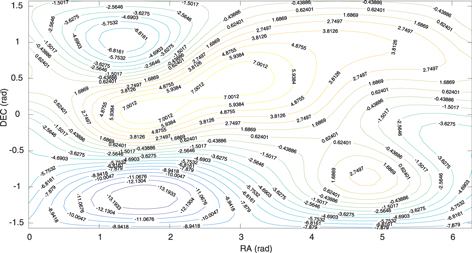
Figure 6. Contour lines corresponding to the potential of the [25, 200] pc slice.
Download figure:
Standard image High-resolution imageTable 20. Singular Points of the Potential and the Vector Fields, Classified by Magnitudes, of the Non-rotational Component. The Singular Points In the Boxes Can be Seen Figure 7
| [25, 200) | Coordinates Type | m4 | m5 | m6 | m7 |
|---|---|---|---|---|---|
| I | (4.7,−0.7) Max | No − KM Source (4.5, −1.05) No − KM Shrink (6.1, −1.15) | Source (4.6, −0.85) |
|
|
| II | (3.5, 0.5) Max | No − KM Source (3.9, 0.2) No − KM Source (4.65, 0.92) | KM Source (3.7, 0.45) | KM Source (4.4, 1) | |
| III | (1.7, 0) Max | KM Source (2.3, 0.2) | (1.75, 0) Source | ||
| (1.3, 1.05) Min | No − KM Shrink (0.85, 1.15) |

|
KM Shrink (0.4, 1.1) | No − KM Source (2.3, 0.5) | |
| IV | (1.7,−1.1) Min | KM Shrink (2.47, −1.02) | No − KM Shrink (1.8, −1.15) | KM Shrink (1.9, −0.95) No − KM Shrink (2, −1) |
Download table as: ASCIITypeset image
Table 21. Singular Points of the Potential and the Vector Fields, Classified by Magnitudes, of the Non-rotational Component. FS Means Faint Source, AF Means Attracting Focus
| [100, 300) | Coordinates Type | m4 | m5 | m6 | m7 |
|---|---|---|---|---|---|
| I | Shrink (5.7, −0.2) | No − KM Source (4.7, −1.1) | (5.9, −0.2) Shrink | ||
| Shrink (5.4, 0.2) | |||||
| II | (3.1, 0.5) Max | KM Shrink (2.8, 0.5) | KM Shrink (5.2, 0.1) | (2.7, 0.3) Source | |
| KM Source (3.75, 0.82) | |||||
| III | (1.5, 0) Max | Shrink (0.9, 1.1) | KM Shrink (1.15, 0.95) | No − KM Source (2.2, 0) | |

|
|||||
| (1.2, 1.1) | |||||
| Min | |||||
| IV | (1.5, −1.25) Min | No − KM Source (1.5, −0.3) | KM Shrink (2, −1.10) |

|
Download table as: ASCIITypeset image
Table 22. Singular Points of the Potential and the Vector Fields, Classified by Magnitudes, of the Non-rotational Component. FS Means Faint Source, AF Attracting Focus, SF Means Source Focus
| [200, 400) | Coordinates Type | m4 | m5 | m6 | m7 |
|---|---|---|---|---|---|
| I | KM Source (5.9, −0.45) | KM Shrink (5.1, 0) | Shrink (6.1, −0.1) | ||
| Shrink (5.7, 0) | No − KM Shrink (5.9, −0.3) | ||||
| No − KM Shrink (5.6, −0.1) | |||||
| II | KM Source (4.8, 0) | No − KM Shrink (5.5, 1.05) | Source (1.9, −0.05) | ||
| No − KM Source (1.9, −0.05) | |||||
| III | (1.2, 1.1) Min |

|
No − KM Shrink (1.4, 1.2) | KM Shrink (1.1, 1.15) | |
| Shrink (1.2, 0.85) | |||||
| F1(1.5, 0) Max | Shrink (1.4, 1.5) |

|
|||
| F2(3, 0.25) Max | KM Source (1.3, 0) | ||||
| Source (1.7, −0.15) | |||||
| IV | (1.5, −1.25) Min | No − KM Shrink (1.7, −1.2) | No − KM Shrink (1.5, −1.25) | ||
| Shrink (1.8, −1) |
Download table as: ASCIITypeset image
Table 23. Singular Points of the Potential and the Vector Fields, Classified by Magnitudes, of the Non-rotational Component. FS Means Faint Source, AF Attracting Focus, SF Means Source Focus
| [300, 500) | Coordinates Type | m4 | m5 | m6 | m7 |
|---|---|---|---|---|---|
| I | (5.9, 0) Min | Shrink (5.8, −0.05) | Shrink (5.8, −0.1) | Shrink (5.8, −0.1) | |
| II | (3.4, 0) Max rel | ||||
| III | (0.5, 1) Min | KM Shrink (2.95, 0.35) | No − KM Shrink (5.1, 1.2) | Shrink (0.1, 1.23) | |
| (1.5, 0) Max | KM Source (1.6, 0.1) | Source (1.9, −0.1) | |||

|
No − KM Source (1.8, −0.1) | ||||
| IV | (1, −1.25) Min |

|
No − KM Shrink (1.4, −1.2) | ||
| No − KM Source (2.5, −0.3) |
Download table as: ASCIITypeset image
Table 24. Singular Points of the Potential and the Vector Fields, Classified by Magnitudes, of the Non-rotational Component. FS Means Faint Source, AF Attracting Focus, SF Means Source Focus
| [400, 600) | Coordinates Type | m4 | m5 | m6 | m7 |
|---|---|---|---|---|---|
| I | |||||
| II | (3.7, 0.3) Max |

|
KM Source (3.8, 0.2) | ||
| III | (0.25, 1) Min | ||||
| (1.7, 0) Max | Source | ||||
| (1.9, −0.05) | |||||
| IV | (1, −1.25) Min |

|
No − KM Shrink (1.5, −0.9) |
Download table as: ASCIITypeset image
Tables 20 to 24 show some additional information with the singular points of the potential for each r and the critical points of the vector fields. We denote as area  , area
  , area
  , and area
We are going to show some examples in which it is appreciated that a maximum of this potential corresponds to a source of the vector field, and a minimum of the potential corresponds to a shrink of the vector field. We recall that the singular points and their situation regarding the critical points of the potential can be seen in Tables 20 to 24. Given that there are many graphs, we have considered it adequate to only show some of the most relevant ones in Figures 7 to 11. Because Tycho-2 was used for the reduction of the 2MASS positions, we studied the surfaces of the BT and VT magnitudes in the neighborhood of the critical points. In a very general way, the VT surface mimics the extrema of the vector field, including the saddle points (these have not been included in the figures because we have selected only a few of them). It should be noted that the surface VT is unique, while vector fields depend on the magnitude, spectral type, and distance, showing patterns—in terms of singular points— that are different in each case.

Figure 7. Slice 25–200. Up, Area III,  , Shrink (1.6, 1); Down, area I,
  , Sources (4.9, −0.8) (and (4.2, −0.75), its corresponding VT surface is not shown). On the left is the potential vector field. On the right is the corresponding VT surfaces.
Download figure:
Standard image High-resolution image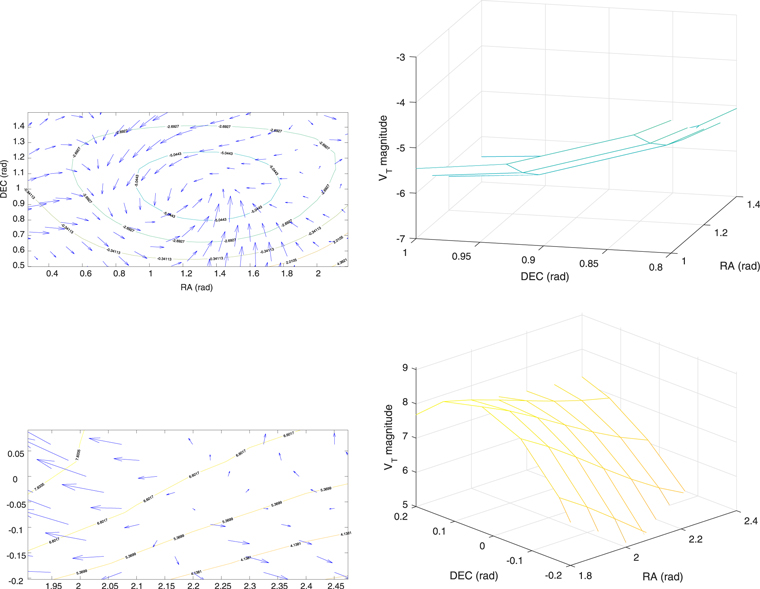
Figure 8. Slice 100–300. Up, area III,  , Shrink (1.3, 0.95); Down, area IV,
  , Source (2.2, 0). On the left is the potential vector field. On the right is the corresponding VT surface.
Download figure:
Standard image High-resolution image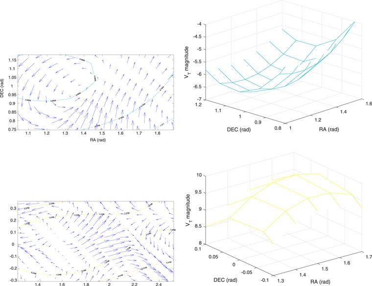
Figure 9. Slice 200–400; Up, area III,  , Shrink (1.4, 0.95); Down, area III,
  , Source (1.5, 0.05). On the left is the potential vector field. On the right is the corresponding VT surface.
Download figure:
Standard image High-resolution image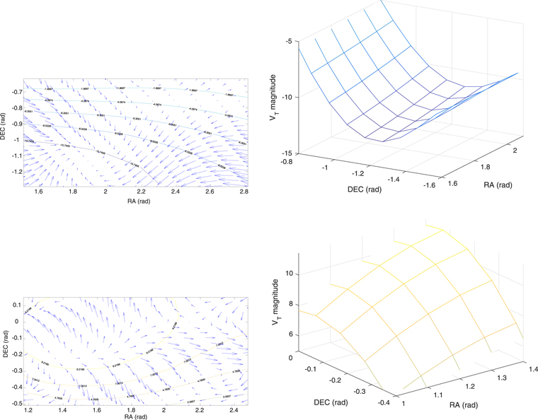
Figure 10. Slice 300–500. Up, area IV,  , Shrink (1.85, −1.1). Down
  , area IV, Source (1.2, −0.2). On the left is the potential vector field. On the right is the corresponding VT surface.
Download figure:
Standard image High-resolution image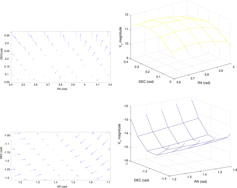
Figure 11. Slice 400–600 Up, area III,  , Source (3, 0.4); Down, area IV,
  , Shrink (1.4, −1.2). On the left is the potential vector field. On the right is the corresponding VT surface.
Download figure:
Standard image High-resolution image
5.3. Application to Obtain Some Proper Motions in the Neighborhoods of the Critical Points
In this subsection, we will consider some of the critical points obtained in the local study, selecting stars around the center within a radius of 0.2 rad. This will provide a number of stars common to Hipparcos and 2MASS in the neighborhood of the selected critical point for each case. We will choose some of them and apply the global correction, depending on the spectral type of the star, its magnitude, and its distance according to TGAS. After these corrections, we follow an elementary process of position improvement; see Marco et al. (2013) and Michalik et al. (2014). As the area of influence is small and we do not aim to obtain a joint solution (this issue will be considered in a further stage), it is not necessary to work with the positions in SMOK coordinates (Michalik et al. 2014). The quotient between the difference of positions (DR1 in t = 2015 and improved version of 2MASS in t = 2000) and the elapsed time for each star provides our approximation for the proper motions (see Table 25) These values are compared with the DR1 values and the PMA values that were obtained from DR1 and amelioration, using another procedure, from the 2MASS catalog. It must be taken into account that star-to-star comparisons are merely indicative. They cannot be representative, in a strict sense, because the adjustments for the elimination of bias are made by minimizing residuals in L2-norm and not in  -norm.
6. Conclusions
In this paper, we have presented a three-dimensional study of the vector field of positional residuals between 2MASS and Hipparcos-2, considering distances from TGAS provided in Astraatmadja & Bailer-Jones (2016b). Such residuals have been used to obtain adjustments by nonparametric regression both for the entire sphere and for slices centered at the distances r = 100, 200, 300, 400, and 500 pc. These regressions have been carried out so that we have obtained the vector fields at equally spaced points. This allows least-squares adjustments from a continuous approach, using integrals, with the exception that these integrals are finally approximated by a numerical integration method. This procedure allows a robust evaluation of the desired parameters. In particular, the spheroidal and toroidal coefficients of the spherical vector harmonic developments that have been applied to vector fields. These have been computed for several cases: (a) all stars, not classified and classified by slices; (b) taking into account if the stars are KM or Non-KM; (c) According to four groups of Hp magnitudes that gather practically all of the stars; (d) Idem with mixtures between KM and different magnitudes, and Non-KM and different magnitudes. We have verified how the coefficients of the vector fields depend on the spectral type and the magnitude, as well as on r. It should be noted that the adjustments have been made by "overlapping" and smoothly, so that the variations of the values of the parameters are also smooth, showing an (intuitive) idea of mathematical continuity. We stress that although the variations, between values of consecutive r, are small, they generally maintain a growing or decreasing tendency, with some exception.
To study the reliability of the results, case (a) (see above) has been applied to 1000 samples created with perturbations times a N (0, 1) for both R.A. and for decl., while for the distance has been considered a perturbation of the 10% of its value times a N(0, 1). The results obtained for the real data are within the confidence interval for each coefficient, obtained by creating the perturbed data in the 1000 samples.
We have considered that the developments of first order for the toroidal component, are sufficient to determine the rotation between both catalogs. On the other hand, we have considered the non-rotational part of the field in more detail. To this aim, the Helmholtz theorem has been used to decompose the vector field in its rotational part (the toroidal components of first order) and non-rotational. Focusing on the non-rotational part and considering that it is the gradient of a potential function, we deduce that the divergence of the residual field coincides with the Laplacian of the potential and that happens for each of the considered cases. If we assume that the potential can be developed in spherical (surface) harmonics, their properties lead immediately to the obtention of the Laplacian of such potential as the sum of coefficients (to be calculated) and the spherical functions themselves. The calculation of the divergence of the residual field is carried out by means of a polynomial local regression of first order, to obtain the first-order derivatives of each component and later the divergence of the vector field. The equality between both members allows, through numerical integration, to obtain the coefficients of the potential. We verify that there are extrema for each potential that correspond to close critical points of the associated vector field. This happens, obviously, in areas of the sphere where the rotational component is small and, therefore, not very influential. From the results included in the tables of Section 5.2, it can be deduced that the patterns of the critical points and the potentials are dependents of r.
Finally, we have taken into account that the 2MASS reductions were made using the Tycho-2 as reference catalog. That is why we have studied the surfaces (here for the whole celestial sphere) corresponding to the magnitudes BT and VT. We have checked that for each critical point of each vector field (in which aspects such as the slice in which we works, the spectral type and the magnitude do have importance) there is a critical point of the VT surface (the case of BT, although in some cases could also be used is, in general, less conclusive). In addition, there is a strong correspondence is between shrinks, sources and saddle points in the vector field and minimum, maximum, and saddle points on the VT surface (see Figures 7–11). Given this and being aware that there are still questions to be answered, we have concluded our 2MASS-Hipparcos-2 residual analysis, is an apparently wide field of work that relates locally the geometry of vector fields to certain physical properties. Notice the importance, which can be seen in the tables and figures of Section 5.2, that the critical points of the surfaces of the magnitude VT are obtained considering the complete celestial sphere, while their relative extrema correspond to critical points of residual vector fields corresponding to a specific subgroup of stars and a certain distance. This confirms the importance of the three-dimensional study introduced and studied in this article.
It is interesting to note that three issues remain. First is the search for a classification by statistical clusters, taking into account at least distances, spectral types, and magnitudes. Second, the improved recent massive catalogs with which to compare different aspects of the Gaia Data Release that are to appear. Third, the Helmholtz decomposition of the velocity field of a catalog, studying the potentials in the different cases in which this vector field is found and seeing the possible implications of the obtained results. It is clear that these issues are to be addressed in later work.
After a simple process of local improvement of the 2MASS stars located in the neighborhood of some of the singular points that appeared in Section 5.2, we have applied the adjustments obtained in Section 5.1 to deduce the induced proper motions and compare them with those provided by DR1 and PMA (see Table 25). It must be neared in mind that the local corrections have not been arranged in the way of a search for a joint solution and that the adjustments we use to minimize the L2-norm, so that the comparison one by one, that is, in the  -norm, should be done with caution and the results are merely indicative.
Table 25.
Comparison between the Proper Motions from DR1, PMA, and Our Obtained Results for Some Stars in the Neighborhood of Some Singular Points of their Vector Field. Hip Stands for the Number of the Star in the Hipparcos Catalog, DR1 for the DR1 Identifier. Subindex (1) means DR1 and (2) Means PMA. The Proper Motions are given in mas, Being the Last Two Columns  μδ Our Obtained Results
| Hip | DR1 | α(1) | δ(1) |

|

|

|

|

|
μδ |
|---|---|---|---|---|---|---|---|---|---|
| 28951 | 1008018207212849024 | 91.6628127275 | 63.4538738263 | −35.558 | 8.594 | −34.73 | 21.84 | −36.35 | 21.33 |
| 30031 |

|
94.7912065760 | 56.5264619828 | −37.640 | −31.332 | ⋯ | ⋯ | −39.10 | −31.05 |
| 24771 | 188796557490084480 | 79.6695937289 | −32.3228506874 | 4.963 | −13.891 | 3.08 | −20.75 | 4.47 | −23.68 |
| 27047 | 4756115082715073920 | 86.0379453784 | −65.1018594755 | −2.259 | 21.541 | −4.01 | 26.0 | −2.24 | 27.01 |
| 23865 | 279443525899748352 | 76.9426318743 | 55.7590984639 | 26.115 | −14.343 | 22.01 | −16.58 | 29.28 | −21.70 |
| 89345 | 6721441368029854976 | 273.4528707722 | −43.2043919512 | −9.007 | −13.989 | −8.55 | −17.27 | −9.91 | −18.69 |
| 44931 | 3841861165533628672 | 137.2857737710 | −1.5880525106 | −27.981 | −35.349 | −28.80 | −45.08 | −23.34 | −43.16 |
| 23863 | 279443525899748352 | 76.9426318743 | 55.7590984639 | 26.115 | −14.3434 | 22.01 | −16.58 | 28.47 | −22.17 |
Download table as: ASCIITypeset image
This paper was partially supported by the UJI-B2016-18, 16I356 project.
Appendix A: Surface Spherical Harmonics
In this Appendix we present the surface spherical harmonics up to fifth order:
Appendix B: Spheroidal and Toroidal Spherical Harmonics Used
Here we include a list of the Spheroidal and Toroidal spherical harmonics used in this paper. The general formulation may be seen in Morse & Feshback (1953). For clarity, we have not included the norms in these formulas: