

Abstract
Spectra of the atmospheric airglow, termed sky spectra, are collected to estimate the total amount of contamination present in science spectra, and are intended to be used in a sky subtraction process. The Sloan Digital Sky Survey (SDSS) and Baryon Oscillation Spectroscopic Survey (BOSS) are large astronomical data sets that have nearly continuously recorded sky spectra at latitude 32.78° N longitude 105.82° W over a duration of 14 years. With a bandpass from 3800 Å to 9200 Å, the BOSS and SDSS airglow spectra contain emission from atomic and molecular oxygen, atomic sodium, and the hydroxyl molecule. The BOSS and SDSS sky spectra are an invaluable long-term record of the variations in airglow emission. Using the BOSS and SDSS sky spectra an analysis of airglow temporal variations was performed. Airglow variations were examined on the three timescales of nightly, annual, and long-term. In this manner the amplitude of airglow temporal variations has been estimated. Coincident satellite observations of the atmospheric profiles in temperature, constituent concentrations, and airglow emissions from the Sounding of the Atmosphere using Broadband Emission Radiometry (SABER) instrument were also examined. The atmospheric profiles were used to gain a deeper understanding of the variations in airglow emission processes as they are observed by ground based astronomical instruments.
Export citation and abstract BibTeX RIS
1. Introduction
Sky spectra are collected to be used in a sky subtraction algorithm to remove unwanted signal from astronomical spectra. The implementation of sky subtraction techniques and their effectiveness have been examined in detail by Wyse & Gilmore (1992), Glazebrook & Bland-Hawthorn (2001), Wild & Hewett (2005), Davies (2007), Ellis & Bland-Hawthorn (2008), and Bolton et al. (2012). The signal observed in sky spectra is the sum of a number of sources such as atmospheric absorption and emission, solar emission, galactic, and extragalactic sources. Authors such as Leinert et al. (1998) or Noll et al. (2012) give a more detailed treatment of all the components comprising background absorption and emission sources. This paper is primarily focused on the atmospheric emission components of the sky spectra.
1.1. Atomic Oxygen
Atomic oxygen is a significant source of energy at the mesopause with a recombination energy of 5.12 eV. Atomic oxygen is produced through the photodissociation of O2 by UV solar radiation in the upper mesosphere and lower thermosphere (MLT) region. Atomic oxygen concentrations are modulated by variations in the transport processes from the upper atmosphere. Shepherd et al. (2004) found that the concentration of O near the mesopause is most significantly modulated by atmospheric dynamics, and both Lindzen (1981) and Xu et al. (2003) demonstrated that O is primarily transported downward through advection and diffusion. Smith et al. (2010) showed that above 83 km the tidal winds account for the full extent of the variation. Atomic oxygen can be long lived in the upper atmosphere at altitudes above the mesopause, and the diurnal population variations are minimal. Allen et al. (1984) compared theory to rocket borne measurements to show that the ground-state atomic oxygen species in the MLT can survive for 6 hours at 85 km, and longer than a month at elevations greater than 100 km. Oxygen profiles measured by Mlynczak et al. (2013a) show that concentrations rapidly decrease to nearly zero at approximately 80 km. Swenson & Gardner (1998) demonstrated that gravity waves were able to create large changes in oxygen concentration in this region because of the steep gradient in concentration.
OI 5,577 Å green line emission is produced in the upper mesosphere and lower thermosphere between 90 and 110 km. Barth & Hildebrandt (1961) were the first to suggest a two-step energy transfer process for the excitation of OI 5577 Å emission:


The reaction in Equation (1) produces excited  precursor through the recombination of atomic oxygen. The excited
  molecule in Equation (2) transfers energy to a ground-state
  oxygen atom raising it to the
  state. Witt et al. (1979) and McDade et al. (1986) confirmed the two-step energy transfer mechanism behind the production of the
  atom, consequently the production of the atom responsible for the green line emission is proportional to the cube of the atomic oxygen concentration.
Bates (1992) and Lopez-Gonzalez et al. (1992) both determined that  was the precursor for
  atom, but later Steadman & Thrush (1994) showed that the
  was the precursor. The excited
  atom spontaneously emits a photon of 5,577 Å in wavelength to relax to the
  state. The spontaneous emission coefficient given by Khomich et al. (2008) is A5,577 = 1.215 s−1 or by Krassovsky et al. (1962) is A5,577 = 1.28 s−1. The spontaneous emission coefficient shows that the
  excited state is short lived, and that transport effects are expected to be negligible.
1.2. Sodium
Chapman (1939) was the first to identify the multi-step excitation process behind the NaD emission. The precursor to the  atom in Equation (4) is the excited NaO* molecule:

Midya & Midya (1993) showed that NaO* is most significantly produced by the reaction in Equation (5):

The NaO* precursor is produced at a rate which is proportional to the local sodium and O3 concentrations:

Thus, the production of the excited sodium atom is proportional to the concentrations of Na, O, and O3:

Sodium and other metals are deposited in the upper atmosphere by meteorites, and meteor ablation occurs at heights near the mesopause. Marsh et al. (2013) found a flux of meteoric material of nearly 100 tons per day. The excited sodium atom,  , is a fine structure doublet state which spontaneously emits through the two transitions in Equations (8) and (9):


The excited sodium atom is very short lived with Krassovsky et al. (1962) reporting spontaneous emission coefficients of A5890 = 6.2 · 107 s−1 and A5895 = 6.2 · 107 s−1, and Khomich et al. (2008) similarly giving A5890 = 6.26 · 107 s−1 and A5895 = 6.26 · 107 s−1.
1.3. Molecular Oxygen
The molecular oxygen emission observed around 8,645 Å is due to the electronically excited O2 molecule. McDade et al. (1986) examined two mechanisms which could produce the electronically excited  molecule. These were a direct process in which the recombination of atomic oxygen forms the excited
  molecule, and a two-step Barth type energy transfer process, but rocket observations by Witt et al. (1979) have shown that direct recombination could not account for the observed population.
The multi-step process examined by McDade et al. (1986) begins with the recombination of atomic O in Equation (10) which provides the initial energy to excite the  precursor molecule:


While McDade et al. (1986) was able to determine the rate of production and removal of the precursor by O and O2, they were not able to identify the excited  precursor itself. Lopez-Gonzalez et al. (1992) theorized that the
  precursor could be the
  state. In Equation (11) a ground-state O2 molecule is excited through a collisional energy transfer with the excited
  precursor. Both Klotz et al. (1984) and Bates (1992) found the lifetimes the
  molecule to be on the order of tens of seconds. Krassovsky et al. (1962) and Bates (1992) list spontaneous emission coefficients of
  and
and  respectively. The
  molecule predominantly radiates through spontaneous emission as in Equation (12).
Sheese et al. (2011) showed that the production rate of the  molecule can be approximated by

where M is primarily O, N2 or O2, and is well approximated by atmospheric densities. The production of the O2 atmospheric emission is proportional to the square of the oxygen concentration. The source of the energy for the excited O2 molecule is the recombination of atomic oxygen.
1.4. OH Molecule
Meinel (1950) was the first to identify the vibrationally excited OH molecule as the source of the infrared emission in the spectrum of the night sky. The reaction in Equation (14),

was originally identified by Bates & Nicolet (1950), and produces vibrationally excited OH molecules in the ninth, eighth, seventh, and sixth vibrational states. Llewellyn et al. (1978) calculated that the nascent distribution of the vibrationally excited OH molecule was populated at approximately 55%, 34%, 7%, and 4% levels, respectively. While Ohoyama et al. (1985) found the nascent distribution to be populated at 32%, 29%, 19%, and 6% levels, respectively.
The ozone hydration reaction in Equation (14) creates vibrationally excited OH through the destruction of O3. The rate of formation of the excited OH molecule near the mesopause is consequently proportional to the O3 concentration, and McDade & Llewellyn (1988) used the reactions in Equation (15) and Equation (16) for the creation of O3:


Smith et al. (2010) assumed that the O3 molecule has a lifetime on the order of a few minutes at altitudes higher than 80 km.
The vibrationally excited OH molecules relax through the spontaneous emission of a photon. Both McDade (1991) and Adler-Golden (1997) demonstrated that collisions with O, O2, and N2 play a significant role in the process of OH vibrational relaxation. OH emission in the optical and near-infrared is from the ground electronic state, which is composed of two sub-states. This multiplet structure, referred to as spin-splitting, is an effect due to the interaction between the electron spin vector and the projection of the orbital angular momentum vector onto the internuclear axis. The F1 rotational states have a total of 3/2 electron spin and orbital angular momentum projected onto the internuclear axis, while the F2 have a projected total of 1/2 angular momentum along the internuclear axis. The ground electronic state of the OH molecule is termed inverted because the energy levels of the F1 states, with higher total angular momentum, are lower in energy than the levels of the F2 states. The emission lines of the F1 transitions are on average three times greater in intensity than the emission lines of the F2 transitions. Transitions between the F1 and F2 states, and vice versa, are rare, consequently they are usually too faint to be observed. The OH emission intensity peaks around 1.5 μm with the Δv = 2 transitions of the first overtone demonstrating the importance of the multi-quantum transitions upon the steady state distribution of the lower vibrational levels.
Each vibrational level of the excited OH molecule is accompanied by a distribution of rotational states. As the vibration and rotation of the OH molecule are coupled vibrational relaxations are often accompanied by a change in the total rotational angular momentum, and are termed ro-vibrational transitions. The selection rules for the rotational transitions are Δj = 0, ±1 giving rise to R, Q, and P branches. The R-branch transitions correspond to Δj = − 1, where Δj = j'' − j'. The Q-branch transitions correspond to Δj = 0, and the P-branch transitions correspond to Δj = +1. For illustration Figure 1 shows a median OH(7-3) spectrum, where the (7-3) notation signifies that the molecule was initially in the v' = 7 vibrational level before relaxing into the v'' = 3 level. The R, Q, and P branches are labeled for reference in Figure 1. The emission lines of the P-branch are more intense than the emission lines from the R and Q-branches an indication that the ro-vibrational transitions preferentially increase the rotational angular momentum of the OH molecule.

Figure 1. Median  spectrum for the SDSS sample of this study (see Sections 1.4 and 2.1 for further details). The Λ doublets are not resolved.
Download figure:
Standard image High-resolution imageThe values in the parenthesis in Figure 1 are N the rotational quantum number, and N' = 1 is the lowest initial total angular momentum state. In the instance of the P1(N' = 1) transition, the final total angular momentum is j'' = 2.5, and final total angular momentum for the P2(N' = 1) transition is j'' = 1.5. The coupling of rotational motion to electronic motion further splits the P1 and P2 transitions. Λ doubling splits each rotational level into e and f components. It takes a very high spectral resolution to be able to resolve any of the Λ doublets.
For an OH molecule in a fixed vibrational level, the populations of low rotational states are assumed to be in thermal equilibrium with the background atmosphere and are well-described by the isothermal Boltzmann distribution given by Cosby & Slanger (2007),
where N0 is the population of the lowest rotational state F1(N = 1),  is the electronic degeneracy for a single Λ doublet line, the 2 · j' + 1 term represents the degeneracy of the rotational states, k is the Boltzmann constant, h is Planck's constant, c is the speed of light, F(j') is the rotational term value of the initial state in units of cm−1, and Trot is the rotational temperature in Kelvins typically around 200 K. The OH molecule is assumed to have achieved a thermal equilibrium between the rotational temperature and the surrounding atmosphere, but a number of researchers such as Cosby & Slanger (2007), Pendleton et al. (1993) and Noll et al. (2015) found that for the higher rotational states there can be significant departures from an isothermal distribution.
Cosby & Slanger (2007) gives the column density of the  state by

where  is the measured intensity of the OH(v' j' ) transition in Rayleighs,
  is the Einstein A coefficient for the particular transition with units of s−1,
  is the initial state, and (v'', j'') is the final state. Rotational temperatures are found by using the slope of a linear fit of
  versus F(j').
Cosby & Slanger (2007) and Noll et al. (2015) only considered the lines from the four lowest total angular momentum states, N = 1, 2, 3, 4, of the P1 and P2 transitions for use in rotational temperature calculations. Cosby & Slanger (2007) excluded lines which were near absorption features, and an inspection of the line atlases by Osterbrock et al. (1996), Osterbrock et al. (1997) or Rousselot et al. (2000) reveal that a few of the OH emission lines are blended with other emission lines. Noll et al. (2015) calculated line specific transmission values to correct line intensities allowing them to reject only the lines which exhibited high optical depths. Emission lines which are effected by absorption or which are contaminated can be a significant source of error in the measurement of the OH rotational temperatures. The affected emission lines will either provide an under or over estimate of the column density of that transition.
The populations of the OH vibrational levels are characterized by the vibrational temperature Tvib. This is not a physical temperature, but rather represents the efficiency of vibrational relaxation. The vibrational temperature is calculated in a similar fashion to the rotational temperature by fitting a line to  versus the total energy of a vibrational transition from the lowest total angular momentum state G(v', 1.5).
OH is produced by the ozone hydration reaction in Equation (14), and Le Texier et al. (1987) showed by deriving Equation (19) that the OH concentration is approximately linearly proportional to the atomic oxygen concentration at low O concentrations,

where  is the rate of ozone production, kQ is the rate of collisional quenching, and
  are the spontaneous emission coefficients. [O] is the atomic oxygen concentration, and [O2] is the molecular oxygen concentration. [M] is the concentration of collisional partners principally composed of either O2 or N2 for which the total atmospheric density is a good approximation. The numerator in Equation (19) represents the rate of production of ozone in Equations (15) and (16), and the denominator represents the loss mechanisms for OH spontaneous emission and collisional quenching.
The largest source of OH emission intensity variations is due to O3 concentration variations at the bottom side of the O3 layer. At elevations near the mesopause Allen et al. (1984) found that the O3 molecule has a lifetime on the order of a few hundred seconds. Nikoukar et al. (2007) found that gravity waves and tides both produce perturbations to the bottom side of the O3 layer due to variations in the O density. The variations in OH emission intensity are are due to changes in chemistry, density and temperature, and Swenson & Gardner (1998) represented the OH emissions response to atmospheric gravity waves (AGW) by Equation (20):
Swenson & Gardner (1998) demonstrated that the greatest variations in OH emission intensity were due to the variations in O concentration. They also found that the perturbations in OH emission intensity from AGW are primarily to the underside of the OH emission layer.
1.5. Aim
This paper has multiple goals. The first is to measure and record the long-term spectroscopic airglow observations contained in Sloan Digital Sky Survey (SDSS) and the Baryon Oscillation Spectroscopic Survey (BOSS) data sets. More detailed information about the SDSS program can be found in Stoughton et al. (2002), and similarly see Dawson et al. (2013) for more information about the BOSS program. These data sets have nearly continuously observed nighttime atmospheric airglow emission since 2000 February from Apache Point Observatory (APO), sunspot, New Mexico, USA, latitude 32.78° N longitude 105.82° W at an elevation of 2,788 m. The duration and large number of observations of these data sets provide the opportunity to examine the temporal behavior of atmospheric airglow over multiple timescales, and to estimate the amplitude of the temporal variations. The second is to better understand the variations in atmospheric airglow which ground based survey instruments observe. Lastly it is important for astronomers to understand the temporal variation of atmospheric airglow to facilitate better sky subtraction algorithms and survey observing plans. This paper is divided into six sections. The introduction concludes here in Section 1. Section 2 details the data sets and data reduction methods used in this work. The following three sections divide the airglow emissions observed in the BOSS and SDSS data sets. First to be analyzed will be the emissions from the atomic lines in Section 3, followed by molecular oxygen emission in Section 4, and lastly OH emission in Section 5. Section 6 is dedicated to the analysis of satellite-based atmospheric profiles observed near APO, and Section 7 is a discussion of the interrelationships between the measurements.
2. Data
Multiple data sets were used in this analysis. Ground based observations were acquired from both the SDSS and BOSS data sets. Nighttime space-based observations from the Sounding of the Atmosphere using Broadband Emission Radiometry (SABER) coincident with the ground based observing site were gathered. The observations used in this study span 14 years. The complimentary observations allow for a deeper investigation into the temporal variations of atmospheric airglow as observed by a ground based instrument.
2.1. SDSS Data
The SDSS spectrograph uses a dedicated 2.5 m f/5 modified Ritchey-Chretien telescope with a 3° field of view. The original spectrograph was operated nearly continuously from 2000 February to 2009 June, but the SDSS telescope typically shuts down for maintenance in July during the monsoon season. The original SDSS spectrograph had a bandpass from 3,800 Å to 9,200 Å with a resolving power, r = λ/Δλ, of approximately 2000. The median SDSS sky spectrum is shown in Figure 2. The SDSS bandpass includes six OH ro-vibrational transitions which are observable: Δv = 7 − 3, 6 − 2, 5 − 1, 4 − 0, 9 − 4, and 8 − 3. The SDSS spectrograph is fiber fed with 640 fibers, and each fiber samples an area of 3 arcseconds in diameter on the sky. A more detailed description of the SDSS telescope and spectrograph can be found in the technical summary by York et al. (2000).

Figure 2. Median SDSS airglow spectrum.
Download figure:
Standard image High-resolution imageA single SDSS telescope observation used fibers to collect 640 spectra simultaneously from which a minimum of 32 spectra were dedicated to astronomically blank patches of sky. The fibers placed on the blank patches of sky are termed sky fibers, and they necessarily sampled points across the entire field of view. The SDSS data set is comprised of 2,880 telescope observations with approximately 100 thousand sky spectra. The average SDSS spectrum is the sum of three 15 minute integration periods. With integration times being much greater than the Brunt-Väisälä period the spectra are not of much use in the study of short scale temporal and spatial variations due to the atmospheric waves. Rees et al. (1990) found that horizontal wind velocities in the mesopause could exceed 100 m/s, and on average were 10 m/s. This implies that in the average 45 minute SDSS integration period, at the average horizontal velocity of 10 m/s, a sky spectrum samples a volume of atmosphere 27 km in length while the entire field of view of the SDSS telescope near the zenith is approximately 4.5 km in diameter at the altitude of the mesopause. Consequently all of the SDSS sky spectra in a single observation are effectively sampling overlapping volumes of atmosphere.
The SDSS spectra are referenced to a heliocentric coordinate system, and before analysis all spectra are shifted into a geocentric frame of reference. Some artificial broadening of the airglow emission lines is expected because each 15 minute exposure has a heliocentric correction applied to the midpoint of the exposure. The airglow lines do not shift in the geocentric frame, but the process of shifting the spectra from the geocentric to heliocentric reference frame introduces small shifts between the centers of airglow emission lines in the final co-added spectrum. In the SDSS data the wavelengths of emission lines are given in vacuum wavelengths. Astronomical spectra are acquired through a range of zenith angles, and the line intensities I(z) were normalized to a zenith observation I(0) using the van Rhijn (1921) conversion:

where h is the height of the emitting layer, assumed to be approximately 87 km, and R is the radius of the Earth. The SDSS spectra are in units of erg/sec/Å/cm2 which for the use in further intensity calculations are converted to units of Rayleighs per Å. Rayleighs have the dimensions of 106 photons/sec/cm2/steradian.
2.2. BOSS Data
The BOSS spectrograph was an upgrade to the original SDSS spectrograph at APO. The BOSS spectrograph has an increased bandpass from 3650 Å to 10,400 Å, with a resolving power of approximately 2000. The number of fibers was increased to 1000, and the diameter of the fibers was decreased to 2 arcseconds in diameter on the sky. The average BOSS spectrum is the sum of four 15 minute integration periods, and the median sky spectrum is shown in Figure 3. The BOSS data used in this work comprised 2599 individual telescope observations totaling nearly a quarter of a million sky fibers. The BOSS observations used in this work were taken from 2009 October through 2017 April. Nearly continuous data were collected through this time, but as with SDSS there are a limited number of observations during July. A more detailed description of the BOSS instrument can be found in Smee et al. (2013).

Figure 3. Median BOSS airglow spectrum.
Download figure:
Standard image High-resolution imageThe BOSS sky spectra, because of the smaller fiber diameter, are at a lower signal-to-noise ratio (S/N) than the original SDSS instrument. The BOSS spectra are similarly referenced to a heliocentric coordinate system, and all spectra are shifted onto a geocentric coordinate system before analysis. Additionally the BOSS spectra are corrected to zenith observations, and have their native units of erg/sec/Å/cm2 converted to Rayleighs per Å.
2.3. SABER
The Thermosphere Ionosphere Mesosphere Energetics and Dynamics (TIMED) satellite was launched 2001 December, and has been continuously monitoring Earth's atmosphere since. The SABER instrument, on board the TIMED satellite, performs limb scan measurements of Earth's atmosphere creating temperature, pressure, density, and volume-emission rate profiles. For a more detailed description of the SABER instrument see Russell et al. (1999). In this work, SABER data version 1.07 was used.
SABER measures atmospheric limb emission in 10 broadband radiometer channels ranging from 1.27 to 17 μm, and atmospheric temperature profiles with a 2 km height resolution are derived from 15 μm CO2 emission measurements. The process which SABER implements for temperature determination is detailed in Mertens et al. (2001). The uncertainties in the SABER CO2 temperature profiles vary from 1% at 80 km to over 20% at 110 km, and Garcia-Comas et al. (2008) determined that the largest single error in the temperature measurements was due to the uncertainty in the quenching rate of CO2 by atomic oxygen. Additional information on SABER's kinetic temperature measurements using CO2 emission can be found in Mertens et al. (2001) or Mertens et al. (2009).
All nighttime SABER observations which began within a 100 km radius of APO were obtained. The atmospheric profiles from SABER are not measured in a strict vertical sense, but instead range over nearly 3° of latitude. The largest variations in atmospheric profiles occur in a latitudinal sense, and the SABER measurements used in this work are intended to measure average atmospheric characteristics at a comparable geographic latitude to APO.
SABER observes OH emission in two bands one centered at 1.6 μm and the second at 2.0 μm, and in this work the filtered data were used. These bands both observe emission from the first overtone, Δv = 2, of the vibrationally excited OH molecule where the emission intensities peak. The emission measured in the 1.6 μm channel is from the OH(5 − 3) and OH(4 − 2) ro-vibrational transitions, and is intended to sample the lower vibrational states. While the emission measured in the 2.0 μm channel is composed of the OH(9 − 7) and OH(8 − 6) transitions sampling the upper vibrational states which are directly populated by ozone hydration. In contrast, the lower vibrational levels are primarily sensitive to the efficiency at which the OH molecule is quenched.
SABER does not directly measure concentrations it measures emission. By measuring the emission intensity and using known or estimated reaction rates a system of chemical reactions can be solved to derive constituent concentrations. The oxygen and hydrogen concentrations are derived from the OH 2.0 μm emission. To measure O and H concentrations Marsh et al. (2006), Smith et al. (2010), and Mlynczak et al. (2013b) rely upon the assumption that nighttime ozone production is in chemical balance with ozone hydration as in Equation (22):

An analysis of SABER H concentrations by Mlynczak et al. (2014) revealed an uncertainty of approximately 35%, primarily due to the rate coefficients kOH and  . Mlynczak et al. (2013b) examined the impact of the reaction rates and quenching parameters upon atomic oxygen concentration retrieval, and found an elevation dependent error which varied from 20% at 80 km to 10% at 110 km.
Ozone emits radiation from 9 to 12 μm due to a bending moment of the linear O3 molecule. The SABER nighttime O3 concentrations are derived from the measurement of the O3 emission near 9.6 μm, and a detailing of this method can be found in Smith et al. (2013). OH and NaD emission are both a consequence of reactions which catalyze the destruction of the O3 molecule. The independent measure of the O3 concentrations provides a mechanism by which to investigate the variations in these emission processes.
2.4. Solar Cycle
The imprint of the solar cycle upon atmospheric emission processes is clear. During periods with increased sunspot numbers there is an excess in UV radiation in the spectrum of the Sun, and it is this energetic UV radiation which is responsible for the photodissociation of molecular oxygen in the thermosphere and the heating of ozone in the stratosphere. The top panel in Figure 4 shows the daily median sunspot numbers from the National Oceanic and Atmospheric Administration found at https://www.ngdc.noaa.gov/stp/solar/ssndata.html. Solar cycle 23 reached a maximum in 2000 March, and ended in 2008 January. While solar cycle 24 began in 2008 January, there were not significant sunspot numbers observed until 2010. The sunspot numbers were characterized by a double peaked maximum in solar cycle 24 with the first peak occurring in late 2011 and the second peak in 2014. The SDSS observations span from 2000 February through 2009 June, capturing the entire decline of solar cycle 23. The BOSS observations began in 2009 September, and continued through 2014 April encompassing the majority of the rise in solar cycle 24.

Figure 4. Upper panel contains the smoothed daily median sunspot numbers; lower panel is the daily median flux at 10.7 cm. The raw timeseries data were smoothed as described in Section 2.5.
Download figure:
Standard image High-resolution imageAnother measure of solar activity is the disk integrated flux at 10.7 cm measured in solar flux units (sfu). The bottom panel in Figure 4 shows the flux at 10.7 cm measured by the Dominion Radio Astrophysical Observatory, and more information on these observations can be found in Tapping (2013). As Hathaway (2010) states the flux at 10.7 cm is a less subjective measure of solar activity than sunspot numbers as it is measured using a radio receiver. The flux at 10.7 cm also has the advantage that it can be measured on cloudy days when the disk of the Sun is not visible.
2.5. Data Analysis
All data analysis performed for this work was done in python using Enthought Python Distribution's (EPD) CanoPy V1.6.1. The primary packages used with CanoPy were NumPy 1.11.3, PyFITS 3.3, SciPY 1.0.0, MatPlotLib 2.0.0, and SciKit-Learn 0.19.1. TeXstudio 2.11.0 was used to type set this manuscript.
To measure individual line intensities the airglow spectra were first oversampled by a factor of four onto a common wavelength sampling. To measure the continuum the spectra were smoothed with a median filter 351 native resolution elements in width. The BOSS and SDSS spectra are sampled with a constant logarithmic dispersion of 69 km/s yielding a resolution of approximately 90 km/s. The width of the filter was selected such that it is wide enough to not be skewed by broad emission features such as the O2 emission or the band heads of OH emission. The measured continuum was subtracted from the airglow spectrum to allow for the measurement of individual lines. All selected airglow lines were measured by fitting a single Gaussian, and integrating the total area under the fitted curve to measure the intensity.
The data used herein were examined for temporal variations on three timescales: diurnal, annual, and the entire duration of the observations. Smoothing of the timeseries data was used as an aid to reveal trends. To analyze the diurnal variations in emission intensities the median normalized BOSS and SDSS data were individually binned into 10 minutes intervals corresponding to the time of night at which integration began, and the median of each bin was calculated. The median was used to remove outliers. A running median filter 5 bins wide, or 50 minutes in width, was used to smooth the data. For the seasonal analysis of emission intensities the daily averages were calculated and smoothed with a median filter 11 days in width. The long-term data are calculated by computing a daily median, and smoothed with a running median filter 31 days in width. The amplitudes of temporal variation are estimated from the smoothed timeseries data, and the values reported are the maximum minus the minimum. These amplitudes are normalized by the median value of the respective BOSS or SDSS timeseries to give a percentage of variation.
2.6. Measurement Errors
The BOSS and SDSS data sets have aperture corrections applied to the raw data to account for the amount of flux the fiber accepts versus the total brightness of the object. These corrections are dependent upon the solid angle subtended on the sky by the fibers. The BOSS fibers subtend 2 arcseconds, and the SDSS fibers subtend 3 arcseconds. Astronomical observations measure the amount of apparent blurring of a point source caused by variations in the optical refractive index by turbulent mixing in the atmosphere, this quantity is referred to as seeing. For the BOSS observations used in this work the median seeing was 1.5 arcseconds with a standard deviation of 0.27 arcseconds, while the median SDSS seeing was 1.6 arcseconds with a standard deviation of 0.42 arcseconds. Assuming the point-spread function (PSF) is well approximated by a double Gaussian of the form used by Bickerton & Lupton (2013) or Title & Berger (1996), the BOSS fiber will accept approximately 60% of the PSF under median seeing conditions, while the SDSS fibers under median seeing accepted 69% of the PSF. The aperture corrections are applied to correct for the flux of a point source which lies outside the diameter of the fiber, but the airglow always overfills the fiber consequently the aperture corrections artificially increase the airglow intensity. In both instances one sigma of variation in seeing represents approximately a 10% change in acceptance. In the case of the median 1.5 arc-second seeing the intensity which the BOSS instrument measures will be approximately 1.2 times that which the SDSS instrument measured. To overcome this deficiency in absolute calibration all flux values have been normalized.
In this work we have made no attempt to undo the aperture corrections as they only affect the absolute calibration, and do not impact our ability to estimate the amplitude of the variations. The variability of seeing does introduce error into the measurements which affect the estimation of the amplitude, but a one sigma change in seeing represents a 10% change in acceptance. The error due to variability in seeing is less than the variations of airglow being quantified in this work.
The Kolmogorov model for turbulence predicts that the seeing scales with wavelength as λ−0.2. Over the bandpass of BOSS and SDSS this represents approximately a 10% change in acceptance. This effect only impacts the absolute measurement, and does not limit the ability to measure the amplitude of variation. No attempt has been made to correct for atmospheric absorption or transmission. These effects may impact some lines used in this work, but they clearly can not have an impact on all of the lines examined.
Fiber-to-fiber variations in a single observation are comprised of instrumental throughput differences, gradients in airglow intensity across the field of view, data reduction errors, and shot noise. In the measurement of the OH emission intensities the standard deviation per observation, the standard deviation of all the fibers from a single pointing, was less than 0.5% for all of the transitions. The standard deviation per observation of the OI 5577 Å emission intensity was less than 0.2% for both the BOSS and SDSS data sets. The larger error in the OH intensity measurement is primarily due to data processing, as eight lines are measured in the OH spectrum versus the single 5,577 Å oxygen line.
The error in the measurement of OI 5,577 Å line is smaller because the line is isolated in the airglow spectrum. The isolation allows for a more accurate continuum removal, and limits contamination for other emission lines. The largest errors in the line measurements in this work are due to errors in the measurement and subtraction of the continuum, and contamination of lines by an adjacent emission line. The standard deviation per observation for all lines considered in this work is less than 0.5%.
While the standard deviation of an observation does not give any measure of absolute error, it is a measure of instrumental and data reduction errors. Distributions of the standard deviation per observation for the OH(6 − 2) and the OI 5577 Å emission intensities are in Figures 41 and 42, respectively, and can be found in the Appendix. The distribution of standard deviation per observation of OH(6 − 2) rotational temperatures has also been included for reference in Figure 43. In Figures 41, 42, and 43 the observation standard deviations have been normalized by their respective observation median to give the variation in terms of a percentage.
3. Atomic Lines
The bandpass of the SDSS and BOSS spectra contain several emission lines from electronically excited atoms. The most prominent atomic emission line is the oxygen OI 5,577 Å green line. Sodium deposited in the upper atmosphere from meteor ablation is responsible for the green NaD doublet observed at 5890 Å and 5895 Å. The OI 6300 Å and 6363 Å red line emission is due to the electronically excited oxygen atom. This work is primarily focused on emission processes occurring near the mesopause, and the oxygen red line emission is not examined because it occurs at higher altitudes in the ionosphere.
3.1. OI 5,577 Å Emission Temporal Variation
The normalized nightly OI 5577 Å intensity variations are plotted in Figure 5. The OI 5577 Å emission increases until local midnight, and then slowly declines until sunrise. Takahashi et al. (1977) in observations taken at 23° S found a similar diurnal behavior. Vyas & Saraswat (2012) measured OI 5,577 Å emission at 35° N, 3 hours before and at local midnight, for a 15 year period, and found the emission intensity to be greater at local midnight. Analyzing 16 years of data observed a 35° N Das et al. (2011) found a diurnal variation on the order of 20% with the maximum occurring near local midnight. In a model by Ward (1999), the migrating diurnal tides drive the vertical transport of atomic oxygen causing the observed variations in OI emission.

Figure 5. Normalized nightly OI 5577 Å emission intensity variations plotted vs. the time of night. The raw timeseries data were smoothed as described in Section 2.5.
Download figure:
Standard image High-resolution imageThe normalized annual OI 5,577 Å intensity variations versus time of year for the BOSS and SDSS data sets are plotted in Figure 6. The OI 5,577 Å emission is maximal in May and October, and the amplitude of the variations in Figure 6 are greater than 50%. In observations taken at 23° S Takahashi et al. (1984) reported semi-annual variations in the OI 5,577 Å emission with maxima occurring in May and November. Clemesha et al. (2005) in observations taken at 23° S saw a semi-annual variation with maxima in April and November. Liu et al. (2008) in observations at 18° N also reported semi-annual variations, but with the greater maximum occurring in the spring rather than the fall. Observing wind patters at 55° N Shepherd et al. (2004) found that the seasonal variations in OI 5,577 Å were correlated to the change in direction of zonal flows around the time of the equinox giving the OI emission intensity variations a semi-annual behavior.

Figure 6. Normalized annual OI 5577 Å intensity variation vs. time of year. The raw timeseries data were smoothed as described in Section 2.5.
Download figure:
Standard image High-resolution imageIn Figure 7 are the normalized long-term OI 5577 Å emission intensity variations of the BOSS and SDSS data sets plotted over the entire duration of observations. Comparing Figure 4 with Figure 7, the impact of the solar cycle on the green line emission is evident. Takahashi et al. (1984) also observed variations in the green line emission correlated to the solar cycle. Using satellite observations Liu & Shepherd (2008) found a linear relationship between the flux at 10.7 cm and green line emission, and they showed that the OI 5577 Å emission intensity has a strong latitudinal dependence characterized by increasing intensity with increasing latitude. The Spearman ρ coefficient was applied to test the significance of the correlation between OI 5577 Å emission intensity and sunspot numbers, and the SDSS observations were significantly correlated with ρ = 0.98, and the BOSS observations were correlated with ρ = 0.81.
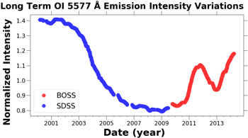
Figure 7. Normalized long term OI 5577 Å emission intensity variations from the BOSS and SDSS data sets plotted vs. time. The raw timeseries data were smoothed as described in Section 2.5.
Download figure:
Standard image High-resolution imageTable 1 lists the measured OI 5,577 Å intensity variations to allow for a quick comparison of the three timescales. The annual variation of the OI green line emission is on the order of 100% of the median, and nightly the OI emission on average varies by 75%, while the solar cycle causes variations in the OI emission on the order of 50%. The nightly and annual temporal fluctuations in the OI 5,577 Å emission observed from the ground are primarily a consequence of the variations in the transport of atomic oxygen.
Table 1. O, O2, and NaD Intensity Variations
| Emission | ΔInightly | ΔIannual | ΔIlong |
|---|---|---|---|
| (%) | (%) | (%) | |
| OI 5,577 Å | 67 | 95 | 39 |
| 72 | 106 | 66 | |
| NaD 5890 Å | 37 | 112 | 30 |
| 34 | 109 | 41 | |
| NaD 5895 Å | 28 | 99 | 20 |
| 16 | 72 | 39 | |

|
51 | 90 | 43 |
| 47 | 84 | 46 | |
Note. Table of variations in emission intensity for the observations of OI 5577 Å, NaD 5890 Å, and 5895 Å, and  emissions. The emission sources are listed on the left. The amplitudes of the temporal variations on nightly, annual, and long-term timescales are listed across the top. The amplitudes of temporal variation are derived from the corresponding plots, and the amplitudes are simply the maximum minus minimum. The values listed are the percentage of the median which the variation represents. The top values listed are the BOSS measurements, and the bottom values are the SDSS measurements.
Download table as: ASCIITypeset image
3.2. NaD 5890 Å and 5895 Å Emission Temporal Variation
Figure 8 is a plot of the normalized NaD 5890 Å and 5895 Å emission intensity variations as a function of the time of night. After sunset the NaD emission intensity rapidly decreases to a minimum, and then slowly increases in intensity until suddenly dropping before dawn. The amplitude of diurnal variation in NaD emission intensity is on the order of 30%.
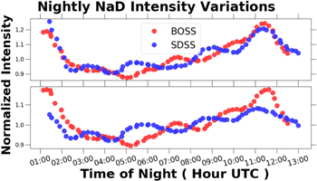
Figure 8. Nightly NaD 5890 Å and 5895 Å emission intensity variations vs. time of night. The raw timeseries data were smoothed as described in Section 2.5.
Download figure:
Standard image High-resolution imageFigure 9 is a plot of the normalized annual NaD 5890 Å and 5895 Å emissions intensity variations. Annually, the NaD emission exhibits semi-annual periodicity, with maxima occurring in April and October, and the NaD emission intensities varied by approximately 100%.
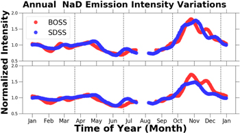
Figure 9. Normalized annual NaD 5890 Å and 5895 Å emission intensity variations vs. time of year. The raw timeseries data were smoothed as described in Section 2.5.
Download figure:
Standard image High-resolution imageThe solar cycle clearly impacts the intensity of NaD emission through the increased production of O and O3. Figure 10 is the plot of normalized NaD emission intensity for the entire duration of the BOSS and SDSS observations. The SDSS observations show a clear correlation to the solar cycle. The SDSS NaD 5890 Å emission intensity variations are correlated to the solar cycle with ρ5890 = 0.9, and the SDSS NaD 5895 Å emission intensity variations are correlated to the solar cycle with ρ5895 = 0.92. The BOSS NaD emission intensity variations are correlated to the solar cycle with ρ5890 = 0.58 and ρ5895 = 0.65.
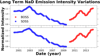
Figure 10. Normalized NaD 5890 Å and 5895 Å emission intensity vs. time for the entire duration of the BOSS and SDSS observations. The raw timeseries data were smoothed as described in Section 2.5.
Download figure:
Standard image High-resolution imageIn Table 1 the sodium emission variations are listed. The NaD emission experiences the most significant variations on annual timescales with variations on the order of 100%. The nightly and long-term variations are both comparable in amplitude with variations in emission intensity on the order of 30%.
3.2.1. NaD Line Ratio
The sodium line ratio is defined as

where I(D2) is the intensity of the 5890 Å emission, and I(D1) is the intensity of the 5895 Å emission. If the  and
and  excited states were produced at a rate corresponding to their statistical spin–orbit weights then the sodium line ratio RD would equal 2. These two data sets represent over 5000 observations of the sodium line ratio spanning over a 14 year duration. The BOSS mean value of RD was found to be 1.55, and for SDSS observations it was 1.5. Slanger et al. (2005) using observations from both the northern and southern hemispheres observed RD to range from 1.2 to 1.8. While Plane et al. (2012) using data collected from multiple sources found RD varied from 1.5 to 2 with an average of 1.67. In Figure 11 are the nightly sodium line ratios RD variations.

Figure 11. Nightly NaD 5890 Å and 5895 Å emission line ratio, RD, variations vs. the time of night. The raw timeseries data were smoothed as described in Section 2.5.
Download figure:
Standard image High-resolution imageFigure 12 is the annual sodium line ratio variations for the BOSS and SDSS data sets. RD achieves a maximum in November, and is minimal in July. Slanger et al. (2005) in observations acquired at 20° N found that the ratio RD was greatest near the equinoxes, and was minimal near the solstices.

Figure 12. Annual NaD 5890 Å and 5895 Å emission line ratio, RD, variations vs. time of year. The raw timeseries data were smoothed as described in Section 2.5.
Download figure:
Standard image High-resolution image4. Molecular Oxygen Emission
The band of emission centered at 8,645 Å is due to the electronically excited O2 molecule, and the median BOSS O2 spectrum is shown in the top panel of Figure 13.
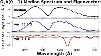
Figure 13. Top panel is the median BOSS  emission; middle panel is the first eigenvector; bottom panel contains the second eigenvector.
Download figure:
Standard image High-resolution image4.1. PCA Eigenvectors
The emission from  transition is not fully resolved in the SDSS spectra, and it is not possible to fit individual rotational lines to measure a rotational temperature. Berg & Shefov (1961) used synthetic profiles in an attempt to estimate the intensity and temperature of the O2 molecule. The
  emission can simply be integrated to quantify the emission intensity, but to gain a deeper understanding of the variations principal component analysis (PCA) was used to generate
  emission eigenvectors.
PCA is used to create a new orthogonal basis to describe the variation in a data set which is comprised of a large number of interrelated variables. The first few principal components will represent the majority of the variation present in the data set reducing the dimensionality. A full description and development of PCA can be found in Jolliffe (2002).
The top panel in Figure 13 is the BOSS median  emission, and the middle panel is the first eigenvector. The first eigenvector represents almost 90% of the variation in the
  emission, and is simply a change in intensity with no variation in shape. The second eigenvector in the bottom panel represents Ca+ absorption, and Noll et al. (2016) found this to be related to the spectra of scattered moonlight, zodiacal light, and scattered starlight. Ca+ absorption accounts for the final 10% of the variation in the
  emission intensity. PCA in this application was able to create eigenvectors which represented both components of variation in the unresolved spectrum of the
  emission.
PCA does not yield any new insight into the rotational temperature of electronically excited O2 molecule. For further analysis of the  emission, a simple integration will be used to measure the intensity of the transition.
4.2. Temporal Variation
Figure 14 is a plot of the nightly BOSS and SDSS  emission intensity variations. A comparison to the nightly variations in OI 5,577 Å emission in Figure 5 shows that the nightly
  emission intensity variations are similar in behavior.
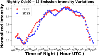
Figure 14. Nightly  emission intensity variations of the BOSS and SDSS data sets. The raw timeseries data were smoothed as described in Section 2.5.
Download figure:
Standard image High-resolution imageThe annual  emission intensity variations in Figure 15 exhibit two maxima which occur during May and October. Lopez-Gonzalez et al. (2004) similarly observed peak
  emission intensities occurring around May and October in observations at 37° N. Gelinas et al. (2008) in observations made at 35° S noted a strong semi-annual oscillation with a weak minimum during the southern summer.
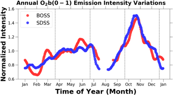
Figure 15. Annual  emission intensity variations for the SDSS and BOSS data sets. The raw timeseries data were smoothed as described in Section 2.5.
Download figure:
Standard image High-resolution imageFigure 16 is a plot of the long term  emission intensity variations in which it can be seen that the solar cycle has an impact upon the emission intensity. The SDSS observations of the
  atmospheric emission are correlated to the solar cycle with a Spearman coefficient of ρ = 0.98, and similarly the BOSS
  emission is correlated to the solar cycle with a correlation coefficient of ρ = 0.84.

Figure 16. Long-term  emission intensity from 2001 to 2014. The raw timeseries data were smoothed as described in Section 2.5.
Download figure:
Standard image High-resolution imageTable 1 and an analysis of the plots in Section 4 both show that the annual variations in the  emission intensity are the most significant with amplitudes on the order of 90%. The nightly and long-term intensity variations are both on the order of 40%.
5. OH Molecule
The emission from the vibrationally excited OH molecule is the most prominent feature in the sky spectra. The band emission of the OH molecule not only allows for the measurement of intensity, but also rotational and vibrational temperatures.
5.1. OH Emission Intensity
The intensities used here are simply the sum of the four lowest angular momentum states, N ≤ 4, of the P1, and P2 transitions neglecting the contributions from other emission lines. The omission of the emission lines from the higher P rotational states is insignificant, but a handful of the lower rotational states from the Q and R branches have intensities comparable to those of the P1 emission lines. Consequently, the integrated intensities measured here underestimate the intensity of the entire band, but the object of this work is to estimate the amplitude of the intensity variations not to measure absolute flux values.
5.1.1. Temporal Variation
The normalized nightly OH emission intensities variations are shown in Figure 17. The OH emission intensity decreases until local midnight followed by a moderate rise until dawn. Noll et al. (2015) in spectra collected at 25° S also observed a steep OH emission intensity decrease at the beginning of the night. In space-based observations of mid-latitudes Gao et al. (2011) found that the OH emission intensity was the greatest after sunset and before sunrise. In Figure 17 a dependence upon vibrational level is also evident. In the evening the emission originating from v' = 4 exhibits the greatest intensity decrease, and the size of this trend is decreasing with increasing vibrational level.

Figure 17. Normalized nightly OH emission intensity variations for the BOSS and SDSS data sets. The raw timeseries data were smoothed as described in Section 2.5.
Download figure:
Standard image High-resolution imageIn Figure 18 each emission intensity has been normalized by its respective annual median emission intensity. The BOSS and SDSS measurements of the normalized annual OH emission intensity variations in Figure 18 exhibit local maxima in May and November. Clemesha et al. (2005) in observations acquired at 23° S and Noll et al. (2015) in observations taken at 25° S both noted semi-annual variations in the OH emission intensity. Marsh et al. (2006) concluded that the observed semi-annual variation in emission intensity was a result of tidal amplitude changes.

Figure 18. Normalized annual OH emission intensity variations for the BOSS and SDSS data sets. The raw timeseries data were smoothed as described in Section 2.5.
Download figure:
Standard image High-resolution imageFigure 19 is a plot of the normalized OH emission intensity variations over the entire duration of the BOSS and SDSS observations. The OH emission intensities observed by SDSS are strongly correlated to the solar cycle with ρ ≈ 0.9, and the BOSS observations were correlated with ρ ≈ 0.8.

Figure 19. Normalized long-term OH emission intensity variations for the BOSS and SDSS data sets. The raw timeseries data were smoothed as described in Section 2.5.
Download figure:
Standard image High-resolution imageTable 2 shows that the annual variations in OH emission intensity are more significant than the nightly variations. OH emission intensities on annual timescales can vary by greater than 50%, and overnight emission intensities vary on the order of 30%. Le Texier et al. (1987) through modeling predicted annual variations in OH emission intensity on the order of 10 to 50%. Over the duration of the SDSS observations the solar cycle intensity decreased by approximately 150 sfu, and the solar cycle intensity increased by approximately 100 sfu during the BOSS observations. The long-term OH emission intensity variations in the BOSS observations were approximately 15%, and for the SDSS observations they were approximately 25%. Noll et al. (2017) found that a 100 sfu change in the solar cycle imparted approximately a 15% variation upon the OH emission intensity.
Table 2. OH Emission Intensity Variations
| Δv | ΔInightly | ΔIannual | ΔIlong |
|---|---|---|---|
| (%) | (%) | (%) | |
| 9-4 | 27 | 52 | 15 |
| 29 | 30 | 25 | |
| 8-3 | 30 | 55 | 16 |
| 35 | 36 | 26 | |
| 7-3 | 26 | 45 | 17 |
| 33 | 30 | 25 | |
| 6-2 | 31 | 46 | 15 |
| 42 | 36 | 25 | |
| 5-1 | 45 | 58 | 15 |
| 45 | 37 | 25 | |
| 4-0 | 49 | 53 | 15 |
| 51 | 38 | 29 | |
Note. Measured OH emission intensity variations from the BOSS and SDSS data sets. The vibrational levels are given at the left. The amplitudes of the temporal variations on nightly, annual, and long-term timescales are listed across the top. The amplitudes of temporal variation are derived from the corresponding plots, and the amplitudes are simply the maximum minus minimum. The amplitudes of variation are the percentage of the median which the variation represents. The top values listed are the BOSS measurements, and the bottom values are the SDSS measurements.
Download table as: ASCIITypeset image
5.2. OH Rotational Temperature
The OH rotational temperatures are a measure of the temperatures near the mesopause. Using the BOSS and SDSS data sets the OH rotational temperatures for transitions originating from the ninth through fourth vibrational levels were measured.
5.2.1. Emission Line Selection
Large high-quality data sets such as the BOSS and SDSS data sets offer a unique opportunity to examine the effect emission line selection has upon OH rotational temperature measurements. For the eight emission lines considered in this work there are a possible 256 combinations in which they can be selected. But since the temperature measurement relies upon the fitting of a line to multiple points the combinations with less than three lines were rejected leaving 219 possible line combinations. OH rotational temperatures were calculated for all of the 219 line combinations, and for each combination of lines a distribution of rotational temperatures was generated. For each combination of lines a median OH rotational temperature was recorded, and emission lines, which variably or systematically improperly quantify column density, will have the effect of decreasing or increasing the median OH rotational temperature of the distribution.
The bottom panel of Figure 20 shows the distribution of median SDSS  rotational temperatures for all 219 emission line combinations. The expected median OH rotational temperature should be approximately 200 K, but the bottom panel in Figure 20 shows that many combinations of lines produced a median rotational temperature closer to 220 K.
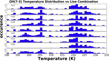
Figure 20. Distributions of median SDSS  rotational temperatures. Each panel represents the distribution of median rotational temperatures derived from line combinations that contain the denoted transition.
Download figure:
Standard image High-resolution imageEach of the other panels in Figure 20 is labeled with a specific rotational transition, and these distributions of median  rotational temperatures are drawn from line combinations which include that specific transition. Clearly, Figure 20 shows that in the calculation of the
  rotational temperature the inclusion of the P2(4) line effectively increases the observed temperature. The P2(4) line has the highest rotational energy of the eight lines investigated in the temperature measurement. Researchers such as Pendleton et al. (1993), Cosby & Slanger (2007) and Noll et al. (2015) have shown that the high rotational energy states of the OH molecule are not in thermal equilibrium.
This analysis suggests that the inclusion of the P2(4) emission line in the measurement of  rotational temperature artificially increases observed temperatures. A rotational temperature could be calculated with as few as two lines from a transition, but using more lines from a transition provide a more robust measure. Other researchers such as Cosby & Slanger (2007) or Noll et al. (2015) based line selection on physical parameters such as atmospheric transmission.
Lines from the  transition such as the P1(4) or P2(1) lines were rejected for temperature calculation because they proved problematic to fit. These transitions often had fitted line widths which were unphysical. The lines used in this work were selected by the statistical analysis of a large number of measurements to reject lines which have a significant amount of fitting uncertainty or consistently skewed rotational temperature measurements.
The same optimization technique in which the  rotational temperatures were calculated for all 219 emission line combinations was performed on the other ro-vibrational transitions in the BOSS and SDSS data sets. The
  ,
,  ,
,  spectra in the BOSS and SDSS observations have good S/N, and the least amount of confusion. Transitions from adjacent overtones overlap, and the emission lines of the
  transition are intertwined with the emission lines from the
  transition. This process yielded the optimal lines with which to calculate OH rotational temperatures, and Table 3 lists the lines which were rejected. The median BOSS and SDSS rotational temperatures listed in Table 4 were measured using the emission line sets in Table 3.
Table 3. Table of Rejected OH Emission Lines
| 7-3 | 6-2 | 5-1 | 4-0 | 9-4 | 8-3 | |
|---|---|---|---|---|---|---|

|
||||||

|
||||||

|
X | |||||

|
X | X | X | X | ||

|
X | X | X | |||

|
X | X | ||||

|
X | |||||

|
X | X | X | X | X |
Note. OH vibrational transitions are listed across the top, and rotational transitions are listed on the left. Emission lines marked with an "X" have been rejected for use in the calculation of OH rotational temperatures.
Download table as: ASCIITypeset image
Table 4. Measured OH Rotational and Vibrational Temperatures
| Temperature | Median | ΔTnightly | ΔTannual | ΔTlong |
|---|---|---|---|---|
| (K) | (K)(%) | (K)(%) | (K)(%) | |

|
201.9 | 14.2 (7) | 21.2 (11) | 6.5 (3) |
| 201.0 | 14.4 (7) | 24.1 (12) | 6.9 (3) | |

|
200.6 | 14.2 (7) | 21.1 (11) | 2.6 (1) |
| 199.7 | 17.7 (9) | 31.2 (16) | 6.6 (3) | |

|
199.1 | 13.2 (7) | 20.1 (10) | 3.0 (2) |
| 197.5 | 14.2 (7) | 24.7 (13) | 6.2 (3) | |

|
195.7 | 14.9 (8) | 22.7 (12) | 2.5 (1) |
| 194.7 | 15.7 (8) | 26.4 (14) | 8.3 (4) | |

|
192.5 | 15.3 (8) | 22.6 (12) | 1.9 (1) |
| 191.7 | 14.7 (8) | 25.3 (13) | 5.6 (3) | |

|
195.5 | 13.0 (7) | 24.3 (12) | 8.0 (4) |
| 194.0 | 20.6 (10) | 28.5 (15) | 9.8 (5) | |

|
11,750 | 1650 (14) | 550 (5) | 350 (3) |
| 11,491 | 2000 (17) | 850 (7) | 250 (2) | |
Note. The rotational and vibrational temperatures are given at the left. The vibrational temperatures are calculated with the 8th vibrational level masked as detailed in Section 5.3. The median temperature and amplitudes of the temporal variations on nightly, annual, and long-term timescales are listed across the top. The amplitudes of temporal variation are derived from the corresponding plots, and the amplitudes are simply the maximum minus minimum. Measured values are in units of Kelvin, and the values given in parenthesis with the amplitudes of variation are the percentage of the median which the variation represents. The top values listed are the BOSS measurements, and the bottom values are the SDSS measurements.
Download table as: ASCIITypeset image
The increased red wavelength coverage of the BOSS spectrograph would at first seem to be welcome. Figure 3 is the mean BOSS sky spectrum, and it has the same OH ro-vibrational transitions as the original SDSS sky spectrum with the addition of the Δv = 9 − 5, 3 − 0 and 8 − 4 transitions. Unfortunately the emission lines from these added transitions are difficult to resolve because of confusion. The 9-5 transition is from the Δv = 4 third overtone, and the 3-0 transition is from the Δv = 3 second overtone. The emission lines from these ro-vibrational transitions overlap leading to contamination.
5.2.2. Einstein A Coefficients
The Einstein A coefficients are considered to be a significant source of uncertainty in the measurement of OH rotational temperatures, and numerous researchers such as Mies (1974), Coxon & Foster (1982), Turnbull & Lowe (1989), Goldman et al. (1998), Cosby & Slanger (2007), Khomich et al. (2008), and Liu et al. (2015) have given a thorough treatment of this topic. In this work the Einstein A coefficients from van der Loo & Groenenboom (2007) are used exclusively, and the rotational term values are taken from the work by Bernath & Colin (2009).
5.2.3. Measured OH Rotational Temperatures
The measured rotational temperatures are given in Table 4 and they show a trend of decreasing rotational temperature with decreasing vibrational level until the fourth vibrational level. The ninth, eighth, and seventh vibrational levels all have median rotational temperatures of approximately 200 K, while the sixth, fifth, and fourth vibrational levels have median rotational temperatures on the order of 195 K. In three years of observations performed at 37° N Lopez-Gonzalez et al. (2004) found the mean  rotational temperature to be 202 ± 6 K. The upper vibrational levels are on average 5 K warmer than the lower vibrational levels. The warmer temperatures of the upper vibrational levels seem to indicate that these levels are farther from local thermodynamic equilibrium (LTE) than the lower vibrational levels. Cosby & Slanger (2007) found a 6 K difference in measured rotational temperatures between the v = 8 versus the v = 6 vibrational levels, and in Table 4 this difference is approximately 5 K. Wrasse et al. (2004) also reported seeing similar differences in rotational temperatures from spectra collected in Antarctica.
5.2.4. Nightly Variation
The nightly OH rotational temperatures all decreased until 03:00 UTC as shown in Figure 21. After 03:00 UTC the rotational temperatures increased until 11:00 UTC when finally showing a sharp decline until sunrise. The amplitude of the diurnal temperature variation is on the order of 15 K for all of the transitions in Figure 21.

Figure 21. Nightly OH rotational temperature variations as a function of time of night. The raw timeseries data were smoothed as described in Section 2.5.
Download figure:
Standard image High-resolution imageFigure 22 is an array of plots showing the overnight differences in measured rotational temperatures using the SDSS data. The difference between rotational temperatures of the upper levels is nearly constant throughout the night, and the difference in rotational temperatures between the lower levels is also nearly constant, but the difference between the upper levels and the lower levels increases until local midnight, and decreases thereafter. Noll et al. (2015) observed that the temperature variations between adjacent vibrational levels were larger for the lower vibrational states.
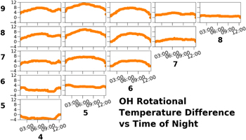
Figure 22. Nightly rotational temperature differences, in units of Kelvins, between vibrational levels from the SDSS data set. The rows and columns are labeled with the upper vibrational level from which the rotational temperature was measured. The raw timeseries data were smoothed as described in Section 2.5.
Download figure:
Standard image High-resolution image5.2.5. Seasonal Variation
The annual rotational temperature variations in Figure 23 achieve a maximum in November and a minimum in June. The annual variations of the OH rotational temperatures are on average 20 K. Takahashi et al. (1995) using observations made at 4° S found annual  rotational temperature variations on the order of 20 K. Lopez-Gonzalez et al. (2004) in observations at 37° N found the OH rotational temperatures varied by approximately 14 K on annual timescales.

Figure 23. Annual OH rotational temperature variations for the BOSS and SDSS data sets. The raw timeseries data were smoothed as described in Section 2.5.
Download figure:
Standard image High-resolution image5.2.6. Long-term Trends
Figure 24 shows the long-term variations in OH rotational temperatures. The most obvious variations in Figure 24 are on seasonal timescales, but the impact of the solar cycle upon OH rotational temperatures is clearly evident. The amplitude of the variations due to the solar cycle are approximately 6 K for all of the vibrational states measured in the SDSS observations. The SDSS observations of OH rotational temperature are correlated to the solar cycle with ρ = 0.98, while the BOSS observations were less significantly correlated with ρ = 0.49. In observations acquired at 51° N, Offermann et al. (2003) also found the OH rotational temperatures to be correlated to solar activity. Offermann et al. (2003) observed a 4.5 K change during the increase of solar cycle 23, which ranged from 70 sfu at its minimum and increased to 220 sfu at maximum. The SDSS data was acquired under a comparable variation in solar activity during the decline of solar cycle 23 and exhibited approximately a 6 k change in rotational temperature. Noll et al. (2017) in observations at 25° S found that all of the OH rotational temperatures varied by approximately 4 K per 100 sfu.

Figure 24. Long-term OH rotational temperature variations. The raw timeseries data were smoothed as described in Section 2.5.
Download figure:
Standard image High-resolution image5.2.7. Temperature Variation
Table 4 summarizes the mean rotational temperatures, and the variations of these temperatures measured on the three timescales of nightly, annual, and long term. The annual variations in OH rotational temperatures are the largest in amplitude at approximately 12%, while the average nightly variation in temperature is about 7%. The solar cycle imparts about a 2% variation upon OH rotational temperatures.
5.3. OH Vibrational Temperature
The median vibrational populations for both the BOSS and SDSS data sets were calculated for the v' = fourth, fifth, sixth, seventh, eighth, and ninth vibrational levels, and the median vibrational temperatures were calculated in the manner described in Section 1.4; these results are shown in Figure 25. The v' = 8 level is overpopulated in Figure 25, and consequently skews the vibrational temperature measurement. Vibrational temperatures were calculated with and without the eighth vibrational level. Inclusion of the eighth vibrational level increased the vibrational temperature by approximately 500 K. The median vibrational temperature for the BOSS data set was 12,096 K, and for the SDSS data set it was found to be 11,531 K.

Figure 25. OH vibrational temperature fit of the median BOSS and SDSS vibrational populations. The labels below the fit line denote the vibrational level.
Download figure:
Standard image High-resolution imageCosby & Slanger (2007) measured an excess in the population of the  vibrational level, and Noll et al. (2015) saw a 40% overpopulation of the v' = 8 level from an isothermal Boltzmann distribution. Khomich et al. (2008) reported cooler vibrational temperatures for v' ≤ 6 vibrational states. The fit lines in Figure 25 are significantly improved when the v' = 8 vibrational level is masked demonstrating that a single temperature may be appropriate after excluding the v' = 8 vibrational level. For the reported vibrational temperatures in this work the v' = 8 vibrational state has been masked in the calculation of the temperature.
5.3.1. Temporal Variation
The nightly vibrational temperature variations are plotted in Figure 26. The vibrational temperature increases by approximately 2,000 K during the first two thirds of the night, and declines by about 1,000 K the last third of the evening. Overnight the BOSS OH vibrational temperatures vary from 11,000 to 12,650 K, and the SDSS vibrational temperatures ranged from 10,750 K to 12,750 K. Noll et al. (2015) in spectra acquired at 25° S also observed that the OH vibrational temperature increased during the night.

Figure 26. OH vibrational temperature variations vs. time of night. The raw timeseries data were smoothed as described in Section 2.5.
Download figure:
Standard image High-resolution imageTo gain further insight into the relationship between the high and low vibrational states the ratios of the vibrational level populations were computed. In Figure 27 is the array of nightly vibrational population ratios plotted as a function of the time of night. The ratio in Figure 27 is defined as high-v to low-v. The population ratios for adjacent levels are nearly flat throughout the night. While the ratio of the upper to lower vibrational levels increases for the majority of the night until sharply declining shortly before dawn. This suggests that quenching of the vibrationally excited OH molecule becomes less efficient as the night progresses.

Figure 27. SDSS OH vibrational population ratios vs. time of night. The ratios are defined as high-v to low-v. All boxes are plotted with equivalent heights centered on the data to allow for comparison. The rows and columns are labeled with the upper vibrational level from which the population was measured. The raw timeseries data were smoothed as described in Section 2.5.
Download figure:
Standard image High-resolution imageThe nightly variations in OH vibrational temperature are three times greater than the annual variations shown in Figure 28. The vibrational temperatures in Figure 28 are minimal at the winter solstice, and achieve a steady maximum for the entirety of the summer. Periods of increased OH vibrational temperature are characterized by decreased OH emission.

Figure 28. OH vibrational temperature variations vs. time of year. The raw timeseries data were smoothed as described in Section 2.5.
Download figure:
Standard image High-resolution imageThe annual vibrational population ratios are shown in Figure 29. While the ratios of adjacent levels are not constant, as in the case of the overnight ratios, they vary significantly less in comparison to the ratios of high to low vibrational levels. The vibrational population ratios vary semi-annually with maxima in May and November, coinciding with the time of year during which the OH emission intensity is maximal.
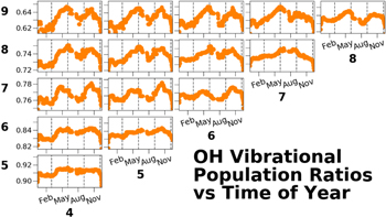
Figure 29. SDSS OH vibrational population ratios vs. time of year. The ratio was defined in the same manner as in Figure 27, and the panels were formatted similarly. The rows and columns are labeled with the upper vibrational level from which the population was measured. The raw timeseries data were smoothed as described in Section 2.5.
Download figure:
Standard image High-resolution image
Figure 30. Long-term BOSS and SDSS OH vibrational temperature measurements spanning 14 years. The raw timeseries data were smoothed as described in Section 2.5.
Download figure:
Standard image High-resolution imageThe long-term OH vibrational temperature variations shown in Figure 30 are significantly influenced by the solar cycle. The SDSS vibrational temperatures were correlated to the solar cycle with ρ = 0.81, and the BOSS observations were correlated with ρ = 0.56. Over the decline of solar cycle 23, the average SDSS OH vibrational temperatures ranged from 11,450 K to 11,700 K. While the BOSS mean temperatures varied from 11,525 K to 11,875 K during the increase of solar cycle 24.
Table 4 lists the measured vibrational temperatures. The largest variations occur on daily timescales with fluctuations on the order of 15%. The amplitude of seasonal variations in the vibrational temperature are approximately 6%, and the solar cycle induced about a 2% variation.
The overpopulation of the eighth vibrational level exhibits variations on both nightly and annual timescales. In Figure 31 the nightly overpopulation variations are shown. The overpopulation is the greatest at the beginning of the night and increases for a short period until smoothly declining until local midnight and remaining steady for several hours. The overpopulations begin to sharply increase again shortly before sunrise.
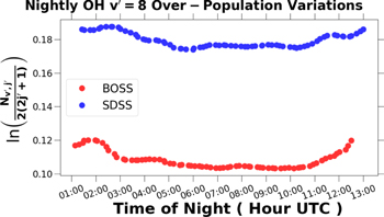
Figure 31. Nightly v' = 8 overpopulation variations vs. time of night. The raw timeseries data were smoothed as described in Section 2.5.
Download figure:
Standard image High-resolution imageThe v' = 8 overpopulation also exhibits significant annual variation shown in Figure 32. The overpopulation increases around the summer solstice, and stays elevated for a significant portion of the summer.
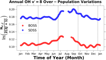
Figure 32. Annual v' = 8 overpopulation variations vs. time of year. The raw timeseries data were smoothed as described in Section 2.5.
Download figure:
Standard image High-resolution image6. SABER Atmospheric Profiles
SABER data V1.07 nighttime observations acquired near APO were used to generate median atmospheric profiles of temperature, O concentration, H concentration, O3 concentration, OH 1.6 μm emission, and OH 2.0 μm emission.
6.1. Nightly Atmospheric Profile Variations
All of the airglow emission sources examined so far originate at or near the mesopause. Common convention defines the mesopause as the temperature minimum at the boundary between the upper mesosphere and the lower thermosphere (MLT). Plane (2003) explains the MLT is of special interest since it directly receives high-energy solar inputs from above, and nearly as much energy due to atmospheric tides and gravity waves from below. Chemical, density, and temperature changes at the mesopause underly the observed variations in airglow intensity. To further examine the observed variations the night was divided into five bins each two hours in width with the middle bin being centered on local midnight from 06:00-08:00 UTC. From the SABER observations median atmospheric profiles were computed for each bin yielding a nightly timeseries.
The left panel in Figure 33 contains the nightly temperature profiles from observations taken with SABER near APO. The temperature profile on average starts early in the night with one minimum near 90 km. As the night progresses a second minimum emerges giving two distinct minima located near 84 and 100 km. Xu et al. (2007) examined the SABER global average thermal structure of the mesopause, and also observed two temperature minima. A lower minimum centered near 82 to 85 km, and a second minimum centered higher near 95 to 102 km. The overnight behavior of the temperature profile exemplifies the dynamic atmospheric variation near the mesopause.
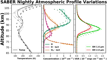
Figure 33. SABER nightly atmospheric profiles observed near APO. The left panel contains the nightly temperature profiles. The second panel contains the concentration profiles for O, O3, and H. The O3 and H concentrations have been multiplied by a factor of 103 to allow for comparison with O concentrations on a single plot. The third panel contains the VER profiles for OH 1.6 μm and OH 2.0 μm emission processes. For each quantity measured the solid line represents the median profile centered on local midnight from 06:00-08:00 UTC. The median atmospheric profiles before local midnight are plotted using dotted lines representing time bins 02:00–04:00 UTC and 04:00–06:00 UTC. The median atmospheric profiles after local midnight are plotted with dashed-dotted lines, and they represent the time intervals of 08:00-10:00 UTC and 10:00-12:00 UTC. The time of observation is also color coded with the color progressing from dark to light as the night progresses.
Download figure:
Standard image High-resolution imageThe second panel in Figure 33 contains the median concentration profiles for O, O3, and H. Early in the evening, the O3 layer shows increased concentrations below 84 km, due to elevated levels of atomic oxygen at these altitudes. Figure 34 is a close-up of the nightly O and O3 concentrations. The inset shows that the O concentrations at 81 km are approximately three times greater in the early evening than at local midnight. The O3 concentrations at 81 km are correspondingly three times larger in the early evening in comparison to local midnight.

Figure 34. Close-up of nightly O and O3 concentration profiles. The formatting of the data is the same as in Figure 33.
Download figure:
Standard image High-resolution imageAfter local midnight the O layer lowers a few kilometers enhancing the O3 concentration above 84 km. The production rate of O3 is inversely dependent upon temperature, and Marsh et al. (2006) estimated that a 20 K reduction in temperature would correspondingly increase the production of O3 by 30%. Since the temperature and O3 number density are simultaneously increasing this implies the source is dynamical in nature. Marsh et al. (2006) observed that variations in O3 concentration, below the altitude of peak concentration, were predominately due to variations of O concentration. While the variations in O3 concentration, above the altitude of peak concentration, were dominated by variations in atmospheric temperature and density.
The third panel of Figure 33 contains the nightly emission profiles for the OH 1.6 μm and OH 2.0 μm emission processes. A comparison of the OH 2.0 μm emission layer in Figure 33 to the O3 concentration in Figure 33 shows that the nightly OH production closely follows the O3 profile. The upper vibrational levels related to the OH 2.0 μm emission layer are directly populated by the ozone hydration reaction in Equation (14), while the OH 1.6 μm emission layer being composed of emissions from lower vibrational states is a reflection of the mechanisms responsible for quenching.
Overnight the integrated OH 2.0 μm VER is nearly constant in intensity, but Figure 33 reveals that the thickness of the layer is decreasing slightly. The upper altitudes of the OH 1.6 μm and OH 2.0 μm emission layers remain at a nearly constant altitude. While contrastingly the location of the bottom halves of the emission layers vary significantly in altitude throughout the night. The early evening factor of 3 increase in O3 at 81 km in Figure 34 directly translates into a factor of three increase in OH emission intensity in Figure 35. Through modeling Swenson & Gardner (1998) determined that the variation of atomic oxygen concentration by AGWs causes significant variations to the bottom of the OH emission layer, but not the top. Similarly, Lyons et al. (2003) also observed that the atmospheric waves primarily caused perturbations to the underside of the OH layer.

Figure 35. Close-up of nightly OH 1.6 and 2.0 μm emission layer profiles. The formatting of the data is the same as in Figure 33.
Download figure:
Standard image High-resolution imagePerforming an analysis similar to Nikoukar et al. (2007) the mean and standard deviation profiles from the observations acquired near APO were computed for the O3 concentration and OH emission, and are shown in Figure 36. The most significant variations to the layers occur below the altitude of peak emission. At the peak of the OH 1.6 μm emission layer the variations are approximately 33%, and the variations at an altitude of 83 km are on the order of 100%. Similarly the OH 2.0 μm emission layer exhibits variations on the order of 33% at the altitude of peak emission, and variations of 100% at an altitude of 83 km. The amplitudes of the variations in O3 concentration and OH emission intensity below altitudes of 83 km are greater than the corresponding mean values leading to large fluctuations.

Figure 36. Mean and standard deviation atmospheric profiles of O3 concentration and OH emission profiles. The mean profiles are marked by solid lines, and standard deviation profiles are marked by dashed lines.
Download figure:
Standard image High-resolution image6.2. Monthly Atmospheric Profile Variations
Using the SABER data collected near APO Monthly atmospheric profiles of temperature, concentrations, and emissions were computed. The same process as in the previous section was applied, but now the nightly atmospheric profile variations were generated for each month of the year. The comparison of these monthly variations at the same local time will enable a further study into the seasonal variations of the chemistry and temperature structure near the mesopause. In Figures 37, 38, 39, and 40 are the monthly atmospheric profiles for January, April, July, and November, respectively. These four months were selected because the OH emission is maximal around April and November, and in July the OH emission is significantly suppressed. January is mid-winter, and was selected to contrast the summertime observations of July. These four months provide observations during the periods of extremes in the airglow emission and atmospheric dynamics. The 60 day orbital precession of the TIMED satellite has caused gaps in the time coverage of the monthly profiles in Figures 37 through 40.
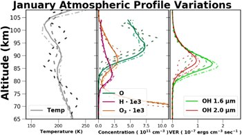
Figure 37. Temperature, concentrations, and emission profiles from SABER for January. The formatting of the data is the same as in Figure 33.
Download figure:
Standard image High-resolution image
Figure 38. Temperature, concentrations, and emission profiles from SABER for April. The formatting of the data is the same as in Figure 33.
Download figure:
Standard image High-resolution image
Figure 39. Temperature, concentrations, and emission profiles from SABER for July. The formatting of the data is the same as in Figure 33.
Download figure:
Standard image High-resolution image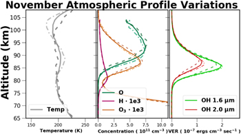
Figure 40. Temperature, concentrations, and emission profiles from SABER for November. The formatting of the data is the same as in Figure 33.
Download figure:
Standard image High-resolution imageFigure 37 contains the January atmospheric profiles. In January, the temperature minima are near their extremes with the upper temperature minimum near its annual coldest around 170 K and the lower minimum is near its annual warmest at 200 K. As the night progresses the bottom side of the O layer lowers in altitude effectively increasing O3 concentrations in this region, and accordingly increasing the OH emission intensity. January, due to the variations in atomic oxygen concentration near the mesopause, exhibits the greatest diurnal variations in OH emission intensity.
The only monthly profile of the four selected to exhibit the early evening enhancement of O3 was April, and is shown in Figure 38. In Section 6.1 it was shown in Figure 34 that the increase in O3 below 85 km was due to an increase in O concentrations at these elevations. The oxygen profile shape evolves significantly over the April night exhibiting increased atmospheric dynamics. The increased dynamics of the April night are able to transport atomic oxygen downward at a rate sufficient enough to maintain higher O3 concentrations below 85 km. Burrage et al. (1995) found that the seasonal variations in emission intensity were caused by seasonal changes in the diurnal migrating tide, and they observed that the amplitude of the diurnal migrating tide is the greatest near the equinox. Both January and April experience significant nightly variation in the thermal structure and composition of the mesopause. In contrast July and November show negligible nightly variation, and the shape of the O layer is nearly constant throughout the night.
July is primarily characterized by suppressed OH emission. This period exhibits increased atomic oxygen concentrations, but situated at higher altitudes in comparison to the rest of the year. Gardner & Liu (2007) observed the greatest vertical winds during June and July in observations made at 35° N. While Thomas (1990) in observations at 40° N observed 4 times the H concentration during the summer in comparison to the spring. In observations taken near APO, July exhibits the greatest annual hydrogen concentrations at altitudes near the mesopause, while contrasting the O3 concentrations are at an annual minimum.
The OH emissions reach their peak intensities during November for which the atmospheric profiles are shown in Figure 40. Both the O and O3 layers peak at their respective minimal annual altitudes during this month, and the O3 concentrations achieve an annual maximum. Increased OH emissions are the direct result of the increased O3 concentrations. The lower temperature minimum peaks at a elevation lower than average around 80 km in November, and achieves its warmest annual temperature of approximately 200 K. The November temperature profile in comparison with January does not exhibit strong diurnal variations.
OH is produced through ozone hydration in Equation (14), and we can see that the rate at which OH is created is dependent upon the H and O3 concentrations near the mesopause. During November, Figure 40, the O3 mixing ratio is at the annual maximum which coincides with the maximum in OH emission. While in July, Figure 39, the O3 mixing ratio is at a minimum, and the OH emission is also at a minimum. An examination of the H mixing ratios shows that they are maximal in July and minimal in November. This demonstrates that the O3 hydration reaction is more sensitive to O3 mixing ratios than H mixing ratios. In fact a further examination of the July mixing ratios shows that an increase in hydrogen is followed by a sharp decrease in O3, but not an increase in OH emission.
7. Discussion
Many of the airglow processes observed in the BOSS, SDSS, and SABER data sets exhibit similar variations. The following discussion is intended to further examine the similarities in these variations on nightly, annual and long-term timescales.
The nightly NaD line ratio variations in Figure 11 are correlated to the nightly OH rotational temperature variations in Figure 21 with ρ ≥ 0.7 for both the BOSS and SDSS observations. Similarly, the annual NaD line ratio variations in Figure 12 are correlated to the annual OH rotational temperature variations in Figure 23 again with ρ ≥ 0.7 for both the BOSS and SDSS observations. A comparison of the nightly NaD emission intensity variations in Figure 8, and the nightly NaD line ratio variations in Figure 11 to the nightly OH rotational temperatures variations in Figure 21 shows the temporal variations of all these processes roughly track together.
A comparison of the nightly OI 5,577 Å emission intensity variations in Figure 5, and the nightly  emission intensity variations in Figure 14 to the nightly OH vibrational temperature variations in Figure 26 shows that the overnight temporal variations of these processes roughly vary together. The nightly OH emission intensity variations in Figure 17 are anti-correlated to the OH vibrational temperature as Noll et al. (2015) had also previously observed.
Comparing the local midnight temperatures at the elevation of maximum OH 1.6 μm emission in July, Figure 39, to the local midnight temperatures in November, Figure 40, there is approximately a 20 K seasonal change in temperature around 87 km which compares well with the variations measured in the annual OH rotational temperature variations shown in Figure 23. The temperature profile in Figure 33 warms 15 K near 87 km over the course of the night, and the OH rotational temperature in Figure 21 also increases by approximately 15 K overnight. The amplitude of the temperature variations observed by SABER, SDSS, and BOSS are all in good agreement.
Comparing the long-term temporal variations over the entire duration of the BOSS and SDSS data sets of all the quantities examined in this work to the flux at 10.7 cm in Figure 4 shows that these processes are all correlated to the solar cycle at some level. This correlation highlights the dependence upon atomic O for all of the airglow processes.
The space-based SABER observations of integrated OH 1.6 μm VERs are the greatest after sunset decreasing steadily until local midnight and then finally slowly increasing until dawn. This is the same nightly behavior observed in the ground based BOSS and SDSS observations of the OH emission intensity variations in Figure 17. The increased intensity of the OH 1.6 μm emission at the beginning of the evening is due to the increased O3 concentrations below 84 km, which are effectively increasing the thickness of the OH emission layer. A three fold increase in O3 at 81 km translated directly into a factor of three increase in OH emission intensity at the same elevation. After local midnight the increase in OH emission intensity occurs at the altitude of peak emission intensity. In Figure 17 it can be seen that before local midnight that the emissions from the lower vibrational levels of the OH molecule experience greater intensity decreases.
8. Conclusion
The BOSS and SDSS data sets combined contain 14 years of nearly continuous nightly spectroscopic observations of atmospheric airglow at a latitude of 33.78° N. The BOSS and SDSS airglow spectra contain contributions from OI 5,577 Å,  , NaD, and OH emission processes. Using this wealth of airglow observations the temporal intensity variations on nightly, annual, and long-term timescales were examined, and the amplitudes of variations for each emission process were estimated. Atmospheric profiles from SABER were compared to the BOSS and SDSS measurements to gain a deeper insight into the observed airglow intensity variations as seen from the ground.
Annually the variations in intensity of the OI 5,577 Å, NaD 5890 and 5895 Å, and  emissions were all observed to be on the order of 100% (calculated as the maximum minus minimum relative to the median). The observed nightly intensity variations of OI 5,577 Å and
  emission were approximately 60%, and the variations in NaD emission intensity were approximately 30%. The observed annual variations in OH emission intensity were approximately 50% for all of the vibrational transitions measured in this work, and on a nightly basis they were observed to vary in intensity by approximately 30%.
The extended duration of the BOSS and SDSS observations show a clear link between atmospheric airglow and the solar cycle. The solar cycle induced intensity variations which ranged from approximately 15% to 65% in amplitude for the emission processes examined in this work.
The variations of OH rotational and vibrational temperatures were also examined on nightly, annual, and long-term timescales. Annually the observed OH rotational temperatures varied by approximately 12%, and nightly they varied by approximately 8%. Contrastingly the observed OH vibrational temperature varied by approximately 15% overnight, and approximately 6% annually. Solar cycle induced variations in OH rotational and vibrational temperatures were at the level of a few percent.
The SABER nightly emission profiles demonstrated that the increased levels of OH emission observed from the ground in the early evening hours are primarily due to an enhancement to the bottom side of the OH emission layer. In the early evening, the OH emitting layer is thicker yielding a longer observed path length through the emission layer for observations made by a ground based astronomical instrument. SABER atmospheric profiles of OH emission shown in Figure 35 demonstrated that the emission intensity at an altitude of 81 km was enhanced by a factor of 3 in the early evening in comparison to local midnight.
Understanding the temporal variations in airglow intensity on the timescales examined in this work will enable astronomers to better apply sky subtraction algorithms or plan observing schedules. The BOSS and SDSS observations provide an insight into the longer timescales over which the airglow vary, and their amplitudes of variation. For astronomers it would also be interesting to know the amplitudes of temporal variation at timescales on the order of a typical integration time of a few hundred seconds. Sampling the airglow on shorter time periods would also allow for an analysis of the spatial scales at which the airglow varies.
The author must first acknowledge the reviewer for the patience and enormous amount of assistance. The reviewer's incredible breadth of knowledge in the subject and related literature was invaluable. Without such gracious help, this manuscript would not have been possible.
We would also thank the TIMED/SABER science teams for providing the atmospheric profile data used in this study.
Funding for the SDSS and SDSS-II has been provided by the Alfred P. Sloan Foundation, the Participating Institutions, the National Science Foundation, the U.S. Department of Energy, the National Aeronautics and Space Administration, the Japanese Monbukagakusho, the Max Planck Society, and the Higher Education Funding Council for England. The SDSS website is http://www.sdss.org/.
The SDSS is managed by the Astrophysical Research Consortium for the Participating Institutions. The Participating Institutions are the American Museum of Natural History, Astrophysical Institute Potsdam, University of Basel, University of Cambridge, Case Western Reserve University, University of Chicago, Drexel University, Fermilab, the Institute for Advanced Study, the Japan Participation Group, Johns Hopkins University, the Joint Institute for Nuclear Astrophysics, the Kavli Institute for Particle Astrophysics and Cosmology, the Korean Scientist Group, the Chinese Academy of Sciences (LAMOST), Los Alamos National Laboratory, the Max-Planck-Institute for Astronomy (MPIA), the Max-Planck-Institute for Astrophysics (MPA), New Mexico State University, Ohio State University, University of Pittsburgh, University of Portsmouth, Princeton University, the United States Naval Observatory, and the University of Washington.
Appendix: Supplemental Plots
While the standard deviation of an observation does not give any measure of absolute error, it is a measure of instrumental and data reduction errors. Distributions of the standard deviation per observation for the OH(6 − 2) and the OI 5577 Å emission intensities are shown in Figures 41 and 42, respectively. The distribution of standard deviation per observation of OH(6 − 2) rotational temperatures has also been included for reference in Figure 43. In Figures 41, 42, and 43, the observation standard deviations have been normalized by their respective observation median to give the variation in terms of a percentage.

Figure 41. Standard deviation per observation of the  emission intensity for the BOSS and SDSS data sets.
Download figure:
Standard image High-resolution image
Figure 42. Standard deviation per observation of the OI 5577 Å emission intensity for the BOSS and SDSS data sets.
Download figure:
Standard image High-resolution image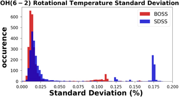
Figure 43. Standard deviation per observation of the  rotational temperature for the BOSS and SDSS data sets.
Download figure:
Standard image High-resolution image