

Abstract
The measurement of Hubble constant (H0) is clearly a very important task in astrophysics and cosmology. Based on the principle of minimization of the information loss, we propose a robust most frequent value (MFV) procedure to determine H0, regardless of the Gaussian or non-Gaussian distributions. The updated data set of H0 contains the 591 measurements including the extensive compilations of Huchra and other researchers. The calculated result of the MFV is H0 = 67.498 km s−1 Mpc−1, which is very close to the average value of recent Planck H0 value (67.81 ± 0.92 km s−1 Mpc−1 and 66.93 ± 0.62 km s−1 Mpc−1) and Dark Energy Survey Year 1 Results. Furthermore, we apply the bootstrap method to estimate the uncertainty of the MFV of H0 under different conditions, and find that the 95% confidence interval for the MFV of H0 measurements is [66.319, 68.690] associated with statistical bootstrap errors, while a systematically larger estimate is  (systematic uncertainty). Especially, the non-Normality of error distribution is again verified via the empirical distribution function test including Shapiro–Wilk test and Anderson–Darling test. These results illustrate that the MFV algorithm has many advantages in the analysis of such statistical problems, no matter what the distributions of the original measurements are.
Export citation and abstract BibTeX RIS
1. Introduction
Nobody disputes the fact that the expanding cosmos is one key finding for human beings. Also, the Hubble constant (H0) is one of the most important constants of physics and astrophysics, and the Hubble's law is the cornerstone of the modern cosmological model. Moreover, the inverse of H0 determines the key value—age of the cosmos (Freedman & Madore 2010). Through accurately determining H0, we can evaluate the expansion rate of the cosmos. For example, Freedman et al. (2001) determined H0 value (H0 = 72 ±8 km s−1 Mpc−1) via Hubble Space Telescope (HST) using high-accuracy distance-measurement approaches, such as Cepheids and Supernova Ia (Riess et al. 1998; Perlmutter et al. 1999; Han & Podsiadlowski 2004; Wang & Han 2012), while Gott et al. (2001) found H0 = 67 ± 3.5 km s−1 Mpc−1 from median statistics on Huchra's compilation.
In order to obtain the more precise value, the methods of measurement of H0 are divided into two major classes (Freedman 2017). One is for measuring the distance, luminosity or size of special astrophysical objects, and the other mainly involves the application of cosmic microwave background (CMB) or large samples of galaxies, associated with the other constants of cosmology. It follows that there are two types of H0 values: ∼72–74 km s−1 Mpc−1 from the object-based observations and ∼67–68 km s−1 Mpc−1 from the CMB-based observations (Jackson 2015). Many key projects in the recent decades have focused on H0, including the HST H0 Key Project (e.g., ∼72 km s−1 Mpc−1 via Cepheid, Freedman et al. 2001), Wilkinson Microwave Anisotropy Probe (WMAP, e.g., ∼70 km s−1 Mpc−1, Hinshaw et al. 2013), large scale surveys of SNe Ia—containing the Supernovae and H0 for the Equation of State of Dark Energy (SH0ES; e.g., 73.24 ± 1.74 km s−1 Mpc−1, Riess et al. 2011, 2016), the Carnegie Supernova Project (CSP; Freedman et al. 2009; Folatelli et al. 2010), baryon acoustic oscillations (BAO; H0 = 67.3 ± 1.1 km s−1 Mpc−1, Eisenstein et al. 2005; Anderson et al. 2014; Aubourg et al. 2015; Cuesta et al. 2016), as well as CMB from Planck, e.g., ∼67 km s−1 Mpc−1, (Planck Collaboration et al. 2011, 2014, 2016a, 2016b).
More recently, other local measurements of H0 with lower central values and bigger error bars (Rigault et al. 2015; Zhang et al. 2017; Dhawan et al. 2018; Fernández Arenas et al. 2018) are more consistent with the median statistics, CMB anisotropy, BAO, and H(z) estimates of H0, which clearly differ from those estimated from Riess et al. (2011, 2016, 2018) at ≳2σ, probably heralding a new non-standard model of cosmology (Freedman 2017). Moreover, the best and most up-to-date summary values for H0 from cosmological (e.g., CMB, BAO, SNIa, H(z), growth factor) data are given in Park & Ratra (2018): H0 = 68.19 ± 0.50 (tilted flat-ΛCDM), 68.01 ± 0.62 (untilted non-flat ΛCDM), 68.06 ± 0.77 (tilted flat-XCDM), and 67.45 ± 0.75 (untilted non-flat XCDM) km s−1 Mpc−1. It should be noted that a lower value of H0 is more consistent with the standard model of particle physics based on three light neutrino species (Calabrese et al. 2012) considering the CMB anisotropy and galaxy clustering data. In addition, Lin & Ishak (2017) performed (dis)concordance tests and supported a systematics-based explanation of considering the higher local measurement as an outlier. Also, favoring the lower value is compatible with recent statistical inference of H0 determined using the Bayesian analyses and Gaussian Processes method (Chen et al. 2017; Gómez-Valent & Amendola 2018; Yu et al. 2018).
The weighted average and median are important ideas to understand the characteristics of different astro-statistical quantities in astrophysical fields. In 2003, Chen et al. (2003) investigated 461 measurements of H0 tabulated by Huchra (See https://www.cfa.harvard.edu/~dfabricant/huchra/) and argued that the error distribution of Hubble constant measurements is non-Gaussian. Furthermore, Chen & Ratra (2011) used median statistics to 553 H0 values compiled by Huchra and provided H0 = 68 ± 5.5 km s−1 Mpc−1 with 95% statistical and systematic errors. Recently, Bethapudi & Desai (2017) applied median statistics to a larger complications of H0 observations including the Huchra records and found  km s−1 Mpc−1. Remarkably, during the past years, many more H0 observations have been obtained along with the better precision. However, there is still a similar non-ignorable gap between the local and global H0 measurements. It is vital to evaluate the true value of H0 considering the consistency of all H0 measurements, which has motivated us to apply the MFV procedure (Zhang 2017) to revisit this problem.
On the other hand, processing observed data to provide astrophysical information is a mutual promotion process which interweaves statistical methods (Feigelson & Babu 2012). One of the most common statistical methods in handling astronomical data is least square method (LSM). Furthermore, linear regression and LSM have derived various algorithms to assess the relationship between astrophysical parameters (Kelly 2007; Hogg et al. 2010; Feigelson & Babu 2012), especially generalized linear methods for the non-Gaussian multivariate analysis (De Souza et al. 2015). However, we have to carefully use LSM on the non-Gaussian distributions of the original measurements (Steiner 1991, 1997).
Another important method is the Bayesian analysis, which is an elegant and powerful approach for estimating the parameters and analyzing the confidence interval in a complicated astrophysical model (Sereno 2016; Chen et al. 2017). Along with investigating the statistical behaviors of enormous variable objects in the cosmos, Bayesian inference approach has obtained considerable improvement in fitting astrophysical model and parameter estimation. For example, Lahav et al. proposed Bayesian hyper-parameters method to estimate the hubble constant from CMB observations (Lahav et al. 2000). However, the calculated conclusions are dependable only if the prior distributions are reasonable for astronomy and astrophysics. Here, for the sake of emphasizing the observed characteristics of sample distributions, we adopt the bootstrap method (Efron & Tibshirani 1994; Davison & Hinkley 1997) to determine the confidence intervals of H0.
As there is a significant tension between measurements from CMB and those from the distance ladder (Bennett et al. 2014), many researchers proposed some cautious assumptions to resolve this problem, e.g., non-standard cosmology (Hamann & Hasenkamp 2013; Battye & Moss 2014; Dvorkin et al. 2014; Wyman et al. 2014). Nevertheless, we cannot rule out the possibility of the statistical fluke and uncharacterized systematics, which needs us to revisit the total data set from the holistic point of view.
In this paper, we apply the MFV method (Steiner 1988, 1991, 1997; Steiner & Hajagos 2001; Kemp 2006; Szucs et al. 2006; Szegedi 2013; Szegedi & Dobroka 2014)—to evaluate H0 value. The MFV technique has been applied in some astrophysical problems presently, e.g., the lithium abundances problem (Zhang 2017). In the next Section we briefly revisit the MFV algorithm. In Section 3, we calculate the MFV and the confidence intervals using the bootstrap method. Moreover, we also discuss the non-Normality of error distribution via the empirical distribution function tests. Conclusions are offered in the final Section.
2. Analysis of Methodology
In astro-statistical fields, the estimation of astrophysical constant from the observed measurements is one of the most vital applications. There are many statistical procedures have been established, e.g., median statistics (Gott et al. 2001; Chen & Ratra 2011; Crandall et al. 2015; Camarillo et al. 2018), maximum likelihood estimation and LSM. However, in general, there is no reason for observers to always suppose that the observed distribution of a physical quantity is necessarily Gaussian. In many situations, normal distribution is not the only choice, even if the sample space is very large. For instance, the most common scenario where the sampling distribution obeys Exponential distribution is irrelative of the size of sample space, when the sample originates from Exponential distribution.
Based on central limit theorem, the distribution of average values of observed sample data should be Gaussian in general. Nevertheless, the error distributions of astronomical data probably are not Gaussian. For example, the observed data may not be a random sample of independent, identically distributed variables (need to test the critical linear combinations of variables), or the observed distribution of data may be heavy-tailed. Apparently, there is no guarantee that the Gaussian feature is invariant for the astronomical data (Chen et al. 2003; Crandall et al. 2015; Singh et al. 2016; Zhang 2017). Similarly, for simple linear regression, one of model assumptions explicitly indicate that the probability distribution of the random component is normal (Mendenhall & JSincich 2011). These difficulties motivate us to consider novel algorithm to reassess H0.
In fact, it is impossible to match perfectly the ideal condition of pure mathematics. Therefore, some necessary assumptions have to be considered to be true, although one knows this is on the ground of expediency, not principle. From the astronomical data, astrophysicists hope to evaluate the influence of different prior distributions. In order to describe the observed data better, a more robust statistical algorithm—MFV has been established by Steiner (1991, 1997), according to the principle of minimization of the information loss. Nearly irrespective of the priori distributions of Gauss or non-Gauss, the MFV keeps high robust efficiency and gets rid of the deficiency, such as high sensitivity for extreme value of big data.
For the sake of clarifying the influence of prior distribution and error distribution, it is necessary to apply the MFV method to evaluate the characteristics of H0 data sets. Different from the maximum likelihood principle or LSM, Steiner proposed maximum reciprocals principle,

where Xi denotes the residuals and deviations, and S is the measurement error. On the basis of the minimization of the information divergence (relative entropy) illustrating the measure of information loss (Huber 1981; Steiner 1991, 1997), Steiner suggested the MFV procedure and the scaling factor ε, i.e., dihesion, with the purpose of assessing the parameter of scale to a certain extent to decrease the information loss. Moreover, the MFV and the dihesion can be calculated through iterations. In the (j+1)th step of the MFV algorithm, the relative equation of iterations for the most frequent value M are as below:

where xi denotes a series of the measurements and the dihesion εj can be obtained by

Here, in beginning step the initial value M0 for the iteration is fixed as the arithmetic mean of the measurements, and the initial value of ε is given as

We can fix the threshold criterion which restrains the precision in iterations. During a series of iterations, the most frequent value M and dihesion ε cannot be obtained until the dihesion is lower than threshold value (e.g., 10−5). Noteworthy, the dihesion ε is not as sensitive as standard deviation in LSM to the outliers.
3. Application to New H0 List
The updated data set of H0 measurements consists of 591 values of H0 (also see Bethapudi & Desai 2017). In much the same way (Chen et al. 2003, Chen & Ratra 2011; Bethapudi & Desai 2017) that the observed errors are not included and the heteroscedastic problem is not considered for the sake of simplicity. Figure 1 demonstrates the histogram and probability density (red line) of all H0 observations. Following the taxonomic approach of Huchra, we have classified all measurements based on primary type. The name and strength of each subgroup are shown in Table 1. The shortcut name is also following Huchra. The calculated results of the MFV are the dihesion ε = 10.372 and H0 = 67.498 km s−1 Mpc−1, which is very approximate to the average value of Planck H0 value of last two years (67.81 ± 0.92 km s−1 Mpc−1 and 66.93 ± 0.62 km s−1 Mpc−1 Planck Collaboration et al. 2015, 2016a, 2016b). Additionally, the corresponding values of subgroup are summarized in Tables 2 and 3 for the MFV and median, respectively.

Figure 1. Histogram and probability density (red line) of H0 observations. For a color version shown in the electronic edition.
Download figure:
Standard image High-resolution imageTable 1. H0: Primary Type Grouping
| Huchra_Type | Types of Estimates | Number | |
|---|---|---|---|
| 2 | = | SnII | 8 |
| A | = | Global Summary | 123 |
| B | = | BTF | 23 |
| C | = | CMB Fit | 21 |
| D | = | Dn-Sig/Fund | 10 |
| F | = | Fluctuations | 18 |
| G | = | GCLF | 14 |
| H | = | IRTF | 19 |
| L | = | Lens | 88 |
| N | = | Novae | 4 |
| O | = | Other | 85 |
| P | = | PNLF | 6 |
| R | = | ITF, RTF | 9 |
| S | = | SnI | 98 |
| T | = | TF | 18 |
| Z | = | Sunyaev-Zeldovich | 46 |
| r | = | Red Giants | 1 |
Note. Huchra_Type is the shortcut for the class name. "Number" is the size of subgroup.
Download table as: ASCIITypeset image
Because the median and average value are not sufficient to reveal the data set of H0 measurements, we make the violin plots to visualize the distributions of the different Huchra Types and their probability density, shown in Figure 2. Every violin plot is a mixture of a box plot and a density plot, whose width denotes the frequency of H0 measurements. The box plot in each violin plot corresponding to different Huchra Type is well-known showing the interquartile range. In particular, the black line in each box plot represents the median, while the green circle denotes the average value.
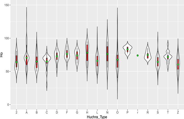
Figure 2. Violin plot of H0 observations.
Download figure:
Standard image High-resolution imageAs is well known, every observed sample is a subgroup and reflects the information of the population. In order to uncover the significant details about distributions of H0 measurements, we especially plot the kernel density plot for the different Huchra Type, shown in Figure 3. Furthermore, the observed distributions of H0 measurements are indicated by circles in Figure 3. Figures 2 and 3 shown as the hybrid plots are particularly useful for comparing summary and descriptive statistics, such as quartiles, median, range and so on.

Figure 3. Density subgroup of H0 observations except Huchra Type is r.
Download figure:
Standard image High-resolution imageIt is reasonably well accepted among astrophysicists that any statistical inference originated from observations is strongly influenced by a certain extent of uncertainty, which restrains us from determining the true value of a given astrophysical object. If astrophysicists can understand well how the prior distributions of the measurements operate, in a sense there remains only a matter of calculation. Given the more robust algorithm to cope with non-Gaussian or Gaussian distribution, the MFV procedure presents a distinctly efficient advantage in the evaluation of H0 (Steiner 1991, 1997).
3.1. Compare with Results of Median Statistics
Chen et al. (2003), Chen & Ratra (2011) applied the median statistics to evaluate H0 and found the non-Gaussian error distribution of H0 measurements. It is very interesting to compare the results by both the median method and the MFV procedure. For Huchra's data set of H0 with 553 measurements, the median is H0 = 68 ± 5.5 km s−1 Mpc−1 (Chen & Ratra 2011), while the MFV is 66.84 km s−1 Mpc−1. At first glance, there can be no doubt that a small difference between the median and MFV seems to exist. However, considering the stability and robustness of results along with increasing data size, we can mitigate greatly this difference. The comparison of results from the median and the MFV over varying time intervals is shown in Table 4.
From the Table 4, if we only consider recent time intervals from 1996 to 2010, there is a negligible difference between the median and MFV. Moreover, it can be seen that the results of the MFV are more stable and robust than that of the median, which fluctuate in a slight vibration range. Clearly, the median is more likely to be influenced by the relative outliers (the values of 1927–1995 years) than the MFV. In addition, the median method yields an integer value of H0 in Table 4, which is inappropriate for a true physical value. Thus, the median can only be considered as the approximate value of H0, while the MFV statistics technique better conforms to the physical and logical rule.
3.2. Confidence Intervals and Bootstrap Method
In observed astrophysical fields, Gaussian statistics has been an important point followed by astronomers with great interests for quite a long time. However, Chen et al. (2003), Singh et al. (2016) and Bailey (2017) have demonstrated that the prior assumptions can not arbitrarily depend on the normality. Clearly, other more robust approaches are needed. It also implies that nonparametric statistics may be the effective method to statistical inference, which does not require the Gaussian assumption.
Different from the classical parametric method, bootstrap method (Efron 1979; Efron & Tibshirani 1994)—one key landmark of nonparametric methods to inference—has made terrific progress. Considering the observational errors for confidence intervals, there is a distribution of the truely exact astrophysical value from the Bayesian point of view. To overcome this uncertainty problem, we would focus on the bootstrap method, which has been widely used by statistician and favorably received by scientists and engineers (Davison & Hinkley 1997).
There are several methods of bootstrap to evaluate the confidence intervals of H0. Because the sample spaces of Huchra et al. do not contain the observational errors of every measurement, we calculate the basic percentile confidence interval in order to estimate the accuracy of measurements (Efron & Tibshirani 1994). Here, it should be pointed out that bootstrap-t confidence interval is not appropriate because of the need to assume the approximately Gaussian bootstrap distribution. Although Romano (1988) investigated the estimation problem of bootstrapping the mode, it is very difficult to theoretically prove the consistency for bootstrapping the MFV due to strikingly difference between the mode and the MFV. On the other hand, from the perspective of the observed heteroscedastic errors, the confidence interval from bootstrap and homoscedasticity is only an approximation, no matter how complicated in mathematic skills. Thus, we adopt the basic bootstrap method to estimate the confidence interval of MFV.
Based on the originally observed data denoting the population, some statistics are used to the measurements. When the statistic is the MFV or the median of sample, the bootstrap approach is contrived as follows. Assuming that the observed data set of H0 is ( ) drawn from the distribution of true value of H0, there are some corresponding statistic
  , such as the median or MFV. First, we create a bootstrap sample
  from the original measurements with replacement. Next, the interesting statistic, i.e., the median or MFV, is applied to the bootstrap sample. Finally, repeating this process B times (typically 1000–3000) leads to the distribution of the median or MFV. As a result, these distributions can be applied to estimate the confidence interval (typically 95%) of the median or MFV for different Huchra Type, shown in Tables 2, 3 and Figures 4, 5, respectively. The 95% confidence interval for all measurements is [66.319, 68.690] involving statistical bootstrap errors, while the corresponding results of the median statistics is [67.8, 70]. In addition, these results also demonstrate the non-Gaussian characteristics of measurements.
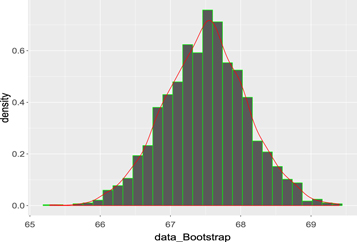
Figure 4. Mfv bootstrap graph of H0 observations.
Download figure:
Standard image High-resolution image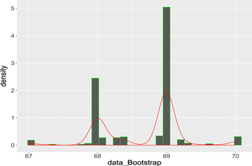
Figure 5. Median bootstrap graph of H0 observations.
Download figure:
Standard image High-resolution imageTable 2. Confidence Intervals of Bootstrap of MFV
| Huchra_Type | MFV | CI.2.5% | CI.97.5% | Range |
|---|---|---|---|---|
| 2 | 58.10 | 54.56 | 76.00 | 21.44 |
| A | 69.92 | 68.42 | 70.81 | 2.39 |
| B | 62.46 | 55.00 | 71.00 | 16.00 |
| C | 70.00 | 65.52 | 70.78 | 5.27 |
| D | 74.85 | 67.00 | 78.51 | 11.51 |
| F | 75.58 | 71.00 | 81.18 | 10.18 |
| G | 75.33 | 68.11 | 80.26 | 12.15 |
| H | 80.65 | 69.15 | 90.80 | 21.65 |
| L | 65.66 | 62.78 | 68.29 | 5.51 |
| N | 76.90 | 56.00 | 95.00 | 39.00 |
| O | 64.22 | 59.32 | 68.40 | 9.08 |
| P | 86.30 | 77.00 | 87.00 | 10.00 |
| R | 73.76 | 69.00 | 80.10 | 11.10 |
| S | 64.05 | 61.78 | 66.30 | 4.52 |
| T | 72.14 | 68.45 | 74.94 | 6.49 |
| Z | 61.50 | 57.25 | 65.50 | 8.25 |
Download table as: ASCIITypeset image
Table 3. Confidence Intervals of Bootstrap of Median
| Huchra_Type | Median | CI.2.5% | CI.97.5% | Range |
|---|---|---|---|---|
| 2 | 59.50 | 55.00 | 76.00 | 21.00 |
| A | 70.00 | 68.90 | 71.00 | 2.10 |
| B | 60.00 | 57.00 | 72.00 | 15.00 |
| C | 69.32 | 67.00 | 70.00 | 3.00 |
| D | 75.00 | 67.00 | 78.00 | 11.00 |
| F | 75.00 | 71.00 | 81.50 | 10.50 |
| G | 76.50 | 68.49 | 79.50 | 11.01 |
| H | 82.00 | 67.00 | 90.00 | 23.00 |
| L | 65.00 | 62.00 | 69.00 | 7.00 |
| N | 77.00 | 56.00 | 95.00 | 39.00 |
| O | 68.00 | 60.00 | 71.00 | 11.00 |
| P | 85.00 | 77.50 | 87.00 | 9.50 |
| R | 74.00 | 69.00 | 82.00 | 13.00 |
| S | 64.50 | 61.00 | 66.50 | 5.50 |
| T | 72.50 | 69.00 | 74.00 | 5.00 |
| Z | 60.50 | 58.00 | 66.00 | 8.00 |
Download table as: ASCIITypeset image
Table 4. The Comparison of Median and MFV Over Varying Time Intervals
| Time Interval | Numbers | Median | MFV |
|---|---|---|---|
| 1996–2010 years | 367 | 67 | 66.86 |
| 1990–2010 years | 426 | 68 | 66.90 |
| 1985–2010 years | 482 | 68 | 66.80 |
| 1980–2010 years | 502 | 68 | 66.93 |
| 1970–2010 years | 534 | 68 | 66.63 |
| 1960–2010 years | 541 | 68 | 66.77 |
| 1927–2010 years | 553 | 68 | 66.84 |
Download table as: ASCIITypeset image
It is a critical problem in physics and astronomy that how to assess the uncertainties in the bias of measurements involving the different subgroups. These systematic bias in different subgroups probably shift the various offsets from the true value (Gott et al. 2001; Chen & Ratra 2011; de Grijs & Bono 2017). Indeed, the accurate analysis of the research on systematic uncertainties to the (non-)independent classification data sets is still very difficult, due to the non-statistical case-by-case characteristics of systematic errors. As described in Chen & Ratra (2011), in order to estimate the systematic bias of subgroup size, the simulation can be completed on basis of different regrouping on numerous occasions. Note that the probabilities in the same subgroup with similar systematic errors are not (more likely) necessarily equal to the probabilities of that among the different subgroups. Therefore, it is reasonable to adopt the bootstrap method to sample the MFV among different subgroups. From the statistical methodology, we do not take account of the Red Giants type containing only one element. The calculated 95% confidence interval of systematic uncertainties is [64.22, 75.47], and  (systematic), while the purely statistical uncertainties can be viewed as the lower limits on the true errors (Gott et al. 2001). Note that this estimated central value has not shifted much from Chen & Ratra (2011) but is still lower than what Bethapudi & Desai (2017) found with the smaller data set.
3.3. Non-normality of Error Distribution
It is worthwhile to note that the distribution of non-Gauss (e.g., heavy tail) may be a common feature of observations in some subjects (Bailey 2017). Even after having considered the interdependent relation between any two measurements, the heavy tail of distribution of measurements still cannot be eliminated completely. Although it is almost impossible to quantitatively, accurately evaluate the covariance between the observed pairs, correlations among observations are very important for the analysis of the observed data in astrophysics and other subjects. This problem is inextricably bound up with the characteristics of the prior distribution of the physical quantities. As is shown by published scientific observations, such distributions may present heavy or small tails on account of the anomalous values or outliers. Suppose the researchers do experiments very carefully and are warranted to be mistake-free, they should record all measurements, which would induce further study on the distribution of true value. Although there is the overestimation or underestimation for uncertainties in big data, it is possible to approach the ideal value in terms of specified statistical method, e.g., the MFV (Steiner 1991, 1997).
Since the statistics was established, the most common means of statistics are built on the basic assumption of Gaussian distribution. However, the astrophysical fact is that non-Normality might be more prevailing in measurements than once thought (Chen et al. 2003; Crandall et al. 2015; Das & Imon 2016). For instance, Singh et al. (2016) used Kolmogorov–Smirnov (K–S) test and pointed out that measurements of Hubble constant show non-Gaussian error distribution in HST Key project Data. There are several tests for normality, such as graphical method, analytical test procedures, supernormality and rescaled moments test (Das & Imon 2016).
Similar to the work of Chen et al. (2003), we construct the residual distribution of the updated compilation of H0. Figures 6 and 7 indicate the absolute magnitude and signed residual distribution of H0 measurements from the central MFV (H0 =67.498 km s−1 Mpc−1), respectively. Meanwhile, Figures 8 and 9 show the absolute magnitude and signed residual distribution from the central median (H0 = 69 km s−1 Mpc−1), respectively.

Figure 6. Histogram of non-Normality of absolute MFV residuals.
Download figure:
Standard image High-resolution image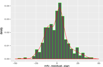
Figure 7. Histogram of non-Normality of signed MFV residuals.
Download figure:
Standard image High-resolution image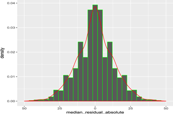
Figure 8. Histogram of non-Normality of absolute median residuals.
Download figure:
Standard image High-resolution image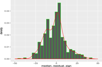
Figure 9. Histogram of non-Normality of signed median residuals.
Download figure:
Standard image High-resolution image
Here, we apply the empirical distribution function test to H0 measurements. A common method is K–S test (Kolmogorov 1933; Smirnov 1948), whose test statistic is

where Fn(X) depends on the observed sample and denotes the empirical distribution function. F(X) is the theoretical cumulative distribution function of the Gaussian distribution (Singh et al. 2016). Note that our goal in this subsection is only to test normality of one-dimension data set instead of estimating the parameters, and applying the K–S test needs to be cautious due to inapplicability in some situations (Feigelson & Babu 2012).
Because the true values (mean μ and variance σ) of H0 measurements are difficult to judge, we have to replace the population parameters (μ, σ) of H0 measurement with the sample estimates. When the sample contains some extreme values, these outliers might influence greatly some sample estimates, such as the average value, and so on. Besides, the observed data set of H0 is a discrete sample. Therefore, for simplicity, we apply the Shapiro–Wilk test (Shapiro & Wilk 1965; Royston 1982, 1995) and Anderson–Darling test (Anderson & Darling 1952; Stephens 1974) rather than K–S test to analysize the normality of measurements. The basic W statistic of Shapiro–Wilk test is calculated as follows:

where the  is the ith ordered sample value and the ai denotes the ith normalized coefficient (Shapiro & Wilk 1965; Royston 1995). The calculated W of absolute residuals from MFV is 0.292 and the p value ≈0, while the W from median is 0.293 and the p value ≈0, too. Obviously, these calculated results demonstrate error distribution of the non-Normality.
It is well-known that the statistic of Anderson–Darling test (Anderson & Darling 1952; Stephens 1974; Das & Imon 2016) is
where ![${\hat{z}}_{i}={\rm{\Phi }}[({y}_{(i)}-\hat{\mu })/\hat{\sigma }]$](https://content.cld.iop.org/journals/1538-3873/130/990/084502/revision1/paspaac767ieqn8.gif) and Φ denotes the standard Gaussian distribution. The calculated A of absolute residuals from the MFV is 236.65 and the p value ≈0, while the A from the median is 234.74 and the p value ≈0, too. Clearly, these results show the rejection of the Gaussian assumption.
and Φ denotes the standard Gaussian distribution. The calculated A of absolute residuals from the MFV is 236.65 and the p value ≈0, while the A from the median is 234.74 and the p value ≈0, too. Clearly, these results show the rejection of the Gaussian assumption.
4. Conclusion
It is essential to determine accurately H0 value in astrophysical fields, especially cosmology. For this reason we apply the MFV procedure to investigate H0 value by the updated complication of 591 H0 measurements, rather than the median statistics. The results of the MFV and bootstrap method are M = 67.498 and [66.319, 68.690] corresponding to 95% confidence interval of statistical bootstrap errors, while that of the systematic uncertainties is [64.22, 75.47]. As can be seen, these results are compatible with the Planck H0 value of last two years according to the ΛCDM model (67.81 ± 0.92 km s−1 Mpc−1 and 66.93 ± 0.62 km s−1 Mpc−1, Planck Collaboration et al. 2015, 2016b) and Dark Energy Survey Year 1 Results (DES Collaboration et al. 2017), which are significantly different from the results of Riess et al. (2016).
The results of the MFV are close to the results of the median statistics, and make up previous shortcoming of integral values of the median method derived from integral data set. This indicates that the MFV procedure is more reasonable and robust. In particular, we introduce the bootstrap method to determine the confidence intervals, which would be a general method for similar astrophysical problems. Obviously, there are an increasing number of examples to demonstrate the advantages of the MFV and bootstrap methods. Moreover, tests for normality of the original observations might be becoming increasingly vital. In short, from the observational and theoretical points of view, acquisition of observed sample data as many as possible is the most important task. Therefore, future research will probably require more measurements of H0 and a better understanding of cosmology.
Author would like to thank the anonymous referee for useful comments and suggestions. J. Zhang acknowledges S. Bethapudi, S. Desai, B. Zhang, Z.-W. Han, H.-Y. Jiang, W. Wei, and Sophia Z. for their kind help about this work described in the paper, and acknowledges the support from the National Natural Science Foundation of China (grant Nos. 11547041, 11403007, 11701135, 11673007), the Natural Science Foundation of Hebei Province (A2012403006, A2017403025) and the Open Project Program of Hebei Key Laboratory of Data Science and Application (No. HBSJQ0701).