

Abstract
PANIC7is the new PAnoramic Near-Infrared Camera for Calar Alto and is a project jointly developed by the MPIA in Heidelberg, Germany, and the IAA in Granada, Spain, for the German-Spanish Astronomical Center at Calar Alto Observatory (CAHA; Almería, Spain). This new instrument works with the 2.2 m and 3.5 m CAHA telescopes covering a field of view of 30 × 30 arcmin and 15 × 15 arcmin, respectively, with a sampling of 4096 × 4096 pixels. It is designed for the spectral bands from Z to KS, and can also be equipped with narrowband filters. The instrument was delivered to the observatory in 2014 October and was commissioned at both telescopes between 2014 November and 2015 June. Science verification at the 2.2 m telescope was carried out during the second semester of 2015 and the instrument is now at full operation. We describe the design, assembly, integration, and verification process, the final laboratory tests and the PANIC instrument performance. We also present first-light data obtained during the commissioning and preliminary results of the scientific verification. The final optical model and the theoretical performance of the camera were updated according to the as-built data. The laboratory tests were made with a star simulator. Finally, the commissioning phase was done at both telescopes to validate the camera real performance on sky. The final laboratory test confirmed the expected camera performances, complying with the scientific requirements. The commissioning phase on sky has been accomplished.
Export citation and abstract BibTeX RIS
1. Introduction
In 2004, the Spanish National Research Council (Consejo Superior de Investigaciones Cientficas; CSIC) and the Max-Planck Society (Max-Planck Gesellschaft; MPG) signed an equal partnership agreement regarding the property and management of the German-Spanish Astronomical Center at Calar Alto (CAHA; Almería, Spain). The 2.2 m and 3.5 m telescopes were a particular focus. Within this agreement, the CSIC and MPG committed to the construction of two new instruments to keep the CAHA instrumentation up to date. The PANIC project started in 2006 July, when the Scientific Advisory Committee of CAHA recommended the construction of a wide-field, general-purpose near-infrared imager for the 2.2 m telescope as the first new instrument.
The project was set up as a collaboration between the CSIC-IAA (Institute of Astrophysics of Andalusia) and MPG-MPIA (Max-Planck-Institut für Astronomie), with the IAA being responsible for the optics and software packages, and the MPIA for the cryogenics, mechanics, detectors and electronics work packages. After the preliminary design phase (Baumeister et al. 2008; Cárdenas et al. 2008), the PANIC concept evolved into a compact (<1100 mm long) and lightweight (<400 kg) near-infrared camera that can be attached to the Ritchey-Chrétien (RC) focus of the 2.2 m and 3.5 m CAHA telescopes. PANIC can take advantage of the maximum field of view (FOV) available at the 2.2 m telescope RC focus without vignetting. The envisaged science comprises many fields, from extragalactic astronomy to the study of the solar system, and the camera is very well suited for survey-type observations.
The final instrument design was described in previous papers (Fried et al. 2010; Cárdenas et al. 2010), including the software system (Ibáñez Mengual et al. 2010) and the characterization and performance of its 4 k × 4 k HAWAII-2RG mosaic (Naranjo et al. 2010). The optics and mechanics final design reports are available through the instrument web pages at CAHA (http://panic.iaa.es/downloads).
The instrument is now finished and was delivered in fall 2014 to its customer, CAHA. PANIC was commissioned at both telescopes in spring 2015. The final construction design was updated with adjustments required by the manufacturing and integration of the instrument. This design is known as the "as-built PANIC". In this paper, we describe the as-built PANIC, with an emphasis on optics, opto-mechanics, detectors, and instrument alignment. A very brief description of the camera appears in Table 1 and the available filters in Table 3.
Table 1. General Capabilities of the 2.2 m and 3.5 m Telescopes RC Foci and a Summary of the PANIC General Performance
| CAHA Telescopes | 2.2 m RC Focus | 3.5 m RC Focus |
|---|---|---|
| Optics | Ritchey-Chrétien | |
| Aperture, ∅ M1 | 2.2 m | 3.5 m |
| Focal length | 17 611 mm | 35 000 mm |
| Focal ratio | f/8 | f/10 |
| ∅ Cassegrain focus | 33 arcmin = 170 mm | 29.5 arcmin = 300 mm |
| Half FOV with no vignetting | 0.275° | 0.245° |
| Scale at Cass. focus | 11.71 arcsec/mm | 5.89 arcsec/mm |
| Max. weight | 400 Kg | >400 Kg |
| Max. length | 1100 mm | >1100 mm |
| System focusing mechanism | Telescope M2 | |
| PANIC Performance | ||
| Direct imaging | Over the whole FOV | |
| Wavelength range | 0.8–2.5 μm | |
| Filters | ZYJHKS and Narrowband ∼1% | |
| FOV | 31.9 arcmin × 31.9 arcmin | 16.4 arcmin × 16.4 arcmin |
| Plate scale | 0.45 arcsec/px | 0.23 arcsec/px |
| Focal ratio | 3.743 | 4.674 |
| Image quality, FWHMa | 0.34 arcsec | 0.17 arcsec |
| Operating temperature | Optics 95 K, Filters 100 K, Detectors 82 K | |
| Cold field stop | Yes | |
| Cold pupil stop | Optimized for 2.2 m | Optimized for 3.5 m |
| Pupil image quality | <2% loss in flux all bands | |
| Distortion | <1.4% (corner) | |
| Transmission | 60% | |
| IR Detector | mosaic of 4 096 × 4 096 pixels, HAWAII-2RG with 2.5 μm cut-off | |
| Gap between detectors, 167 pixels | 75 arcsec | 40 arcsec |
Note.
aFull Width at Half Maximum.Download table as: ASCIITypeset image
2. As-built PANIC
PANIC operates at temperatures around 100 K (detectors at 82 K) and is cooled by liquid nitrogen (LN2). The optical design was modeled and optimized for operation temperatures of 95 K (filters at 100 K) and vacuum environment. The mechanical design, manufacturing, and assembly was done at room temperature (300 K). In the following, we refer to the cold (100 K) and warm (300 K) models.
The final theoretical design of the camera does not completely match the real instrument for two reasons. First, the optical elements are specified with a certain tolerance and, after they are manufactured, they are measured with high accuracy and then re-introduced into the optical model with real, final values. Second, to reach optimum performance, re-machining of parts and final adjustments were required during instrument alignment and integration. These actions produced the "as-built opto-mechanics". After these steps, the real dimensions and shapes of the optical and opto-mechanical elements were entered into the optical design to produce a more realistic model. This common procedure results in the so-called as-built model.
In this section, we present a summary of the camera requirements and performance, and we describe the as-built instrument.
2.1. Overview of the as-built PANIC
Table 1 presents an overview of the as-built PANIC performance. Images of PANIC installed at the 2.2 m and 3.5 m telescopes during commissioning appear in Figure 1.
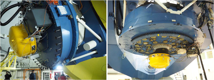
Figure 1. PANIC installed at the 2.2 m telescope, including the electronics rack attached below the telescope main mirror cell (left) and at the 3.5 m telescope (right).
Download figure:
Standard image High-resolution imageThe camera technical requirements demanded a compact and lightweight instrument that could be attached to the RC focal station of both telescopes. The limits in weight and size are set by the 2.2 m telescope. In addition, the requirements stated that the flexure of the instrument shall not degrade optical quality, as the standard guiding unit on the telescope cannot be used because it would vignette the PANIC FOV.
PANIC is optimized for the Z, Y, J, H, and KS bands, and it was initially equipped with these five broadband filters plus two narrowband filters (H2, 2.118 μm and Br-γ, 2.191 μm). The filter wheels can accommodate a further eight filters. The optical design incorporates cold field and pupil stops to reduce the thermal background. Special care was taken in the selection of the infrared materials for the optics to maximize the instrument image quality and throughput over its complete wavelength range. The main challenges of this design are:
- –Producing a well-defined and mechanically available internal pupil, which allows for the reduction of thermal background with a cryogenic pupil stop;
- –The correction of off-axis aberrations due to the large FOV;
- –The correction of chromatic aberration due to the wide spectral coverage; and
- –The capability of using narrow band filters (Δ λ/λ) in the system.
The last requirement is driven by the need to minimize the degradation in the filter passband without a collimated beam, as no collimated beam was required in the camera.
2.2. Optics
The camera optical design is a folded single optical train with nine lenses and three folding mirrors that images the sky onto the focal plane at a focal ratio of f/3.74 and a plate scale of 0.45 arcsec per 18 μm pixel (at the 2.2 m telescope RC focus). This pixel scale allows us to cover almost the maximum FOV of the telescope without vignetting. The mosaic of four HAWAII-2RG detectors (see Sections 2.8 and 3) gives a FOV of 30 × 30 arcmin (with 0.45 arcsec/pixel) at the 2.2 m, and 15 × 15 arcmin (with 0.225 arcsec/pixel sampling and f/4.67) at the 3.5 m telescope. Figure 2 shows the unfolded optical path, which is 1890 mm long from the entrance window to the detector. It also shows the actual folded solution.
To use PANIC at the 3.5 m telescope, a custom-made cold pupil stop is the only additional element required. The PANIC optical design provides a mechanically accessible pupil image8 between L5 and L6 (see Figure 2), where a cold pupil stop wheel is located. This wheel contains two cold pupil stop masks, each of them optimized in size and position for one telescope. In addition, an adapter, which ensures the same focal position when instruments designed for the 2.2 m are mounted on the 3.5 m, was already available at CAHA.
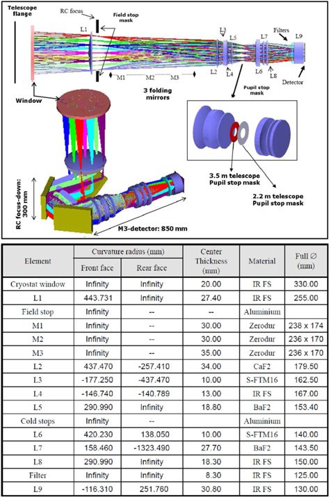
Figure 2. PANIC optical layout, including the unfolded layout (top) and the optical components prescription data at warm (bottom).
Download figure:
Standard image High-resolution imageThe camera optical train consists of one field lens, L1, close to the telescope focus and two separate groups of lenses. The first group (L2 to L5) sits before the cold pupil stop wheel, and the second (L6 to L9) is after that wheel. There are two lens barrels, LM2 and LM3, which comprise lenses L2 to L5 and L6 to L8, respectively. The filters are introduced in the space between L8 and L9 where the effects of the camera focal ratio and the change in the incidence angle with field over the filter are smaller.
At the filters, there is a Pupil Imager Lens (PIL) that can be introduced into the optical path. This images both the pupil stop mask and M1 simultaneously on the detector. This is an engineering tool used to properly align the pupil stop mask for each telescope. There is another engineering tool: the exit window. This window is built into the PANIC cryostat just behind the detector location. Whenever the detector is not installed, the light from the entrance window goes through all the PANIC optics and exits through the exit window. This was used for the alignment of the complete opto-mechanical axis in the laboratory at cold temperatures. After this alignment, this window was removed and the flange was sealed.
The optics packaging solution introduces three folding flat mirrors in the optical path between L1 and L2 (see Figure 2). A cold field stop is placed at the RC focal plane, just after L1, providing shielding from off-axis light sources that are outside the desired FOV. This cold field stop mask is common to both telescopes.
The optics material choice was based in the chromatic correction and the low absorption in the wavelength range of interest. In addition, we used glasses with existing experimental data of their refractive index and coefficient of thermal expansion (CTE) at cryogenic conditions. A glass catalog at 95 K was produced ad hoc to model the system at working conditions.
Because the camera is mounted at warm temperatures and operates cold, internal mechanical mounts are required not only to ensure the survival of the optical elements due to differential thermal expansion of the lens and mount materials, but also to allow the lenses to return to their original positions after warmup or cooldown. The lens-mount concept implemented in PANIC has proved to work correctly in other instruments such as Omega2000, which has big lenses with similar dimensions to PANIC (Baumeister et al. 2003), and as ALFA (Costa et al. 2004; Bizenberger et al. 2005). Baumeister et al. (2003) describes the mounting scheme in detail. In essence, the lenses have 40° polished chamfers on both outer edges (see in Figure 3 the PANIC lens 8). They are mounted in aluminum mounts having the same kind of chamfer. The lenses sit on the conical surfaces of the mount and there is a retainer ring that keeps the lenses in this position. Temperature variations result in changes on the diameter of the parts. These changes lead to an axial displacement of both the lenses and retainer rings because the parts can slide on the chamfer surfaces in relation to each other, but it keeps the optical axis unchanged. On the one hand, this configuration compensates the mismatch of thermal expansion between the lens and the mount material, allowing the lenses to move in their mounts while the instrument cools down and warms up. On the other hand, the lens maintains the axial alignment between warm and cool.
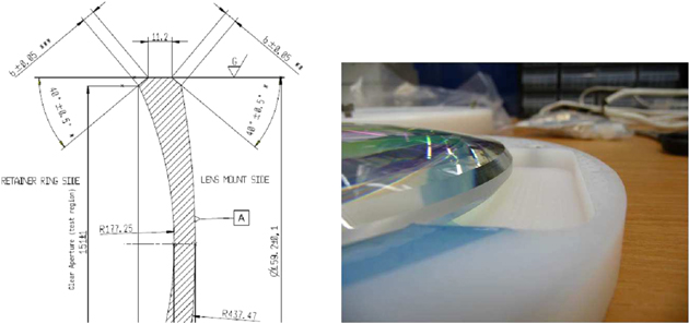
Figure 3. PANIC lenses: example of the chamfers specification in lens 3 drawing (left), and chamfers manufactured in lens 8 (right).
Download figure:
Standard image High-resolution imageThis mechanical mount forces several mechanical requirements on the lens geometry and the chamfer quality. The chamfers are made at a 40° angle have a minimum length of 4 mm and are manufactured with high precision (see Figure 3). They are polished like an optical surface, reducing the friction between the glass material and the aluminum. This aspect had a big impact on the optical design because it drove a minimum thickness on the edges of all lenses for the chamfers to be machined. The prototype of these chamfers was tested in a real mount and was cryogenically cycled with success (see Figure 4).
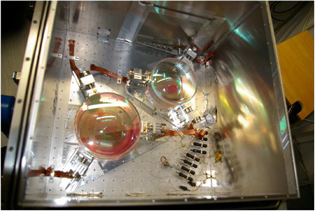
Figure 4. Lens 3 and lens 6 inside the test cryostat after a cryogenic cycle.
Download figure:
Standard image High-resolution imageThe as-built parameters were measured at room temperature for all optical elements and they were then calculated for cold conditions. The translation from warm optical parameters to cold has two aspects. The first is the materials' shrinkage, which is derived using the CTE. This calculation affects not only the optical materials but also the materials used for the opto-mechanics (the spaces between the lenses, in particular, are aluminum Al-5083-T6). The second aspect is the variation in refractive index, which depends on both wavelength and temperature. Therefore, we modeled the lenses at 95 K and the filters and PIL at 100 K. The optical cold model was updated with these cold as-built parameters. For the lenses, these parameters are the radii, thicknesses, wedges, and chamfer sizes; for the L3 and L6 lenses the refractive indices of the S-FTM16 glass blanks are also introduced. The wedges and chamfer sizes of the PIL are included as well. For the entrance window, we include the flatness, thickness, and refractive index. For the filters, the parameters are the thicknesses and the passband at working conditions (see Table 3).
The optical error budget was built with a compensation strategy that allows for the relaxation of some critical values in position and tilt of the optical elements as well as meeting the performance required by introducing compensators in LM2 and LM3. Two types of compensators are implemented: the distance between lenses (Z-compensators) and the decentering of individual lenses. They are later explained in Sections 2.4 and 4.2, Lens barrels. Concerning the Z-compensators, there are two in PANIC: one is the distance between L2–L3 by moving L3 inside the LM2, and a second one in LM3 with the L7–L8 distance, by moving L8. The retrofit of the optical model with the as-built optics and the as-built opto-mechanics was made. Then the distance between those lenses was re-optimized with the aim of relaxing as much as possible the tolerances for the next stages and to determine them for the final system's mounting. With regards to the decentering compensators, there are also two of them: in LM2 by L2 and in LM3 by L6. Once the barrels LM2 and LM3 are assembled, those lenses can be adjusted in the two directions perpendicular to the optical axis in order to achieve the best optical alignment of each barrel.
The following actions were taken in PANIC to minimize the stray and scattered light into the instrument:
- (a)The field and pupil stops are implemented as mentioned previously in this section.
- (b)All of the lenses have been over dimensioned over their clear aperture to avoid stray light coming from the lens edges, including the effects due to the lens chamfers.
- (c)Every opto-mechanical module (see Section 2.4 "Opto-mechanics") is light-tightened.
- (d)Implementation of baffles inside the optical path based on an stray light and ghosts analysis.
- (e)The folding mirrors are gold coated on a glass substrate (instead of metal) to reduce imaging errors and scattered light.
- (f)No optical element with diamond turned surfaces (i. e. aspheric surfaces) has been used to minimize the surface micro-roughness contribution to the total scattering.
- (g)All of the aluminum parts directly visible to the optical beam are blackened with black anodizing.
The aluminum machined parts were sand blasted prior to anodizing. This technique produces a surface with the lowest total reflectivity for black anodized aluminum (Marshall et al. 2014).
2.3. Filter Wheel Unit and Filters
PANIC has a filter wheel unit comprising four wheels with six positions each. Wheel #1 is toward the telescope and wheel #4 is toward the detector. The final configuration is listed in Table 2; Figure 5 shows wheel #1 as an example.
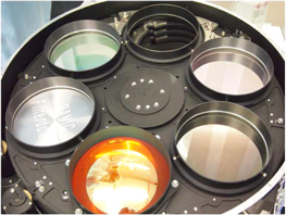
Figure 5. Telescope side of the filter wheel #1 in its final configuration. It is filled with filters J (top left), Y (top right), H (bottom right), the PIL (bottom), and a "Blank" (bottom left). The open position is on the top.
Download figure:
Standard image High-resolution imageTable 2. Final Configuration of the PANIC Filter Wheels. The Science Filters are in Bold. The Dummies Can be Removed and Replaced with New Filters, if Necessary
| Position | |||||||
|---|---|---|---|---|---|---|---|
| 1 | 2 | 3 | 4 | 5 | 6 | ||
| Wheel | 1 | Y | H | PIL | Blank | J | Open |
| 2 | Z | KS | Blank | H2 | Dummy | Open | |
| 3 | Dummy | Dummy | Blank | Dummy | Dummy | Open | |
| 4 | Dummy | Dummy | Blank | Dummy | Br-γ | Open | |
Download table as: ASCIITypeset image
The filters have clear aperture diameters of 11.4 cm and are located in a converging beam. Therefore, it is not possible to combine two filters on different wheels, due to the change in the optical path length. The manufacturing specifications of the filters are driven by two factors:
- 1.The filters are in a converging beam (here we encounter two effects: the camera focal ratio and the change in the incidence angle with field over the filters) and
- 2.The working temperature is 100 K.
With regards to 1.), the expected filter performance of interference filters will suffer a broadening of the apparent bandpass, a depression of transmittance values and a shift to shorter wavelengths. With regards to 2.), a shift to shorter wavelengths.
The PANIC filter set has been specified and manufactured taking into account the corrections of those effects, specially for the narrowband filters.
Five broadband and two narrowband filters are installed. The PANIC Z, Y, J, and H bandpasses match those of the filters of WFCAM (Hewett et al. 2006), the KS bandpass is shifted 0.04 μm to the blue wavelengths. Their as-built parameters in working conditions (100 K and converging beam) are listed in Table 3: center wavelength, FWHM, cut-on and cut-off wavelengths at 50% of the maximum transmission, all in microns, as well as their in-band average transmission for the broadband filters and peak transmission for the narrow ones. The out-of-band blocking density is at a minimum optical density of four in the range 0.3–3.5 μm, except for the Z filter which is blocked until 3 μm. The red leaks of all bandpass filters are located at wavelengths beyond 3 μm, where the detectors are not sensitive any more. Figure 6 shows the transmission curves in working conditions for all the filters installed, as well as the theoretical atmospheric transmission of the CAHA sky9 . The transmission curves are available in electronic form on the instrument web pages (http://panic.iaa.es/instrument).
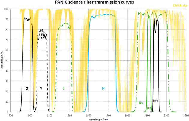
Figure 6. PANIC filter transmission curves in working conditions (100 K and converging beam) including the theoretical atmospheric transmission at CAHA altitude.
Download figure:
Standard image High-resolution imageTable 3. PANIC Filters as-built Parameters in μm at the Working Conditions (100 K and Converging Beam)
| Filter | λa | Δλb | Cut-on 50% | Cut-off 50% | T |
|---|---|---|---|---|---|
| Z | 0.874 | 0.106 | 0.821 | 0.927 | 85% |
| Y | 1.023 | 0.105 | 0.971 | 1.075 | 75% |
| J | 1.247 | 0.157 | 1.169 | 1.326 | 84% |
| H | 1.638 | 0.285 | 1.495 | 1.780 | 93% |
| KS | 2.150 | 0.328 | 1.986 | 2.314 | 95% |
| H2 | 2.118 | 0.034 | 2.101 | 2.135 | 93% |
| Br-γ | 2.191 | 0.055 | 2.163 | 2.218 | 83% |
Notes.
aλ, center wavelength. bΔ λ, FWHM.Download table as: ASCIITypeset image
The filter wheel unit also includes the PIL, one aluminum blank element in each wheel for dark exposures, and eight mass dummies. The PIL, located in wheel #1, has been optimized for usage in the K band wavelengths, therefore the KS and the H2 filters are placed in wheel #2. Dark exposures should be taken with the blanks in all wheels simultaneously preventing photon leakage from outside into the inside of the instrument. Dummies can be removed to install new filters upon request.
2.4. Opto-Mechanics
The baseline design for the opto-mechanics has been directly derived from the folded optical design, including baffles. Figure 7 shows an overview of the optical bench with all elements installed and it also shows the camera in its laboratory caddy. The optics are grouped in several parts that are individually adjustable in position and tilt. The structural layout can be split into a tree structure (see Figure 8) starting at the telescope. The cryostat is attached to the telescope adapter (TA). Inside, the cold optical bench carries the individual optics mounts (OM) 1 and 2. Connected to OM1 are the mirror structure (MS) and the cold pupil stop wheel (CSW) housing. The MS is equipped with the three folding mirrors M1, M2, M3 and the lens mount 1 (LM1), which holds lens 1 (L1). The CSW housing carries the LM2 barrel with lenses 2–5 in front of the pupil stop wheel. The second optics mount, OM2, carries only the filter wheel (FW) housing. Attached to it are the LM3 barrel, with lenses 6–8 in front of the filter wheels, and LM4 with L9 behind the filters. At the end, the detector (focal plane array; FPA) is mounted to OM2. All of the elements are mounted to the bench to minimize flexure effects. The modules are light-tightened to minimize the stray light. PANIC has no focusing mechanism of its own, as focusing is done with the telescope secondary mirror. A highly critical design aspect is the small tolerances, of the order of 50 μm, imposed by some optical elements. The mounting method uses chamfers at both outer edges of the lenses (see Section 2.2). Each lens can be aligned individually at warm in its mount with fine thread screws which are removed after alignment. To achieve the required tolerances, the lens groups are attached directly to the CSW and FW housing, respectively. This results in a more elaborate design of the housings but reduces the number of mechanical interfaces. Generally, several smaller parts are integrated to a group using dowel pins and fitting diameters. This ensures a good positional accuracy. Those groups are then integrated into the next higher level using adjustment devices in position and tilt to compensate the remaining mechanical tolerances and to ensure maximum optical performance.

Figure 7. Left: PANIC optical bench with detectors and optics installed. Light enters from below and is directed to the main optical elements in the back of the bench. At the telescope, the instrument will be attached upside-down compared with this view. Right: PANIC cryostat with its laboratory caddy at CAHA after transportation and reassembly.
Download figure:
Standard image High-resolution image
Figure 8. Mechanical structures with nested groups, from bottom up: telescope; cryostat; cold optical bench; optics mounts (OMs); mirror structure (MS) and wheel housings; lens mounts (LMs); and individual lenses, mirrors, wheel elements, and focal plane array (FPA). The OM1 and the OM2 interfaces are adjustable with shims and movable pins for the alignment of the opto-mechanical axis. The field stop mask is installed in LM1.
Download figure:
Standard image High-resolution imageThe Z-compensators in each barrel were implemented in lenses L3 and L8 at this stage by means of a ring between L2–L3 and another ring between L7–L8, respectively, which are re-machined to the final calculated distances. The decentering compensators were implemented in L2 and L6 (see Section 2.2). Those lenses can be shifted in the two directions perpendicular to the optical axis by using fine thread screws. The adjustment unit consists of two rings with parallel flat surfaces (one for each adjustment direction, X and Y) which allow the attached lens to slide along this surface.
To achieve a sufficiently low weight, all larger parts were light-weighted according to deflection analysis simulated by finite elements analysis at several zenith distances. The goal was to reduce as much material as possible within the given tolerances. Inside the cryostat, only aluminum was used to avoid conflicts with different CTE rates. The cryostat itself is also made of aluminum. The adapter between telescope and instrument is made of carbon fiber to make it as light as possible. By design, the complete opto-mechanics system shrinks with respect to the cold plate center. Then the actual opto-mechanics axis was measured at cold and the parts were positioned accordingly as explained in the Section 4.2.
2.5. Mechanisms
PANIC is equipped with two mechanisms, which are the only moving parts in the camera: one cold pupil stop wheel and one filter wheel unit. The former contains two aperture stops or masks for the different pupils at the two telescopes. The latter consists of four separate filter wheels on a common axis in one housing (see Section 2.3). The CSW is turned by an individual stepper motor via a gearbox. The FW is driven directly at its disc perimeter. The positions are recorded by hardware switches in the housing, triggered by cams mounted on the wheels. A filter configuration change takes a minimum of 5 s (best case) and a maximum of 25 s (worst case) to be executed.
2.6. Cryogenics
A bath cryostat is used to cool the instrument. The diameter of the cryostat is about 1100 mm. To save weight, we did not use the widespread nested tanks design. Thermal drifts due to changes in the nitrogen level and movement of the instrument on the optical bench are of the order of 10 K, which is acceptable for the optics but not for the detector. Therefore, a second small vessel is dedicated to cool down the detectors mosaic to about 80 K (this small tank can be clearly seen in Figure 7; it is the aluminum tank behind the FW unit and close to the FPA). This temperature is held constant within ±0.1 K and it is actively controlled to keep such stability by its own temperature control. The detector tank refilling is required every two days.
The cryostat cooldown and warmup have become routine operations after multiple executions for the laboratory tests, and runs without problems. From room temperature and atmospheric pressure, it takes about 1 day to reach vacuum conditions and about 4–5 days to reach working temperatures. The instrument can then be operated without external pumps, while an internal sorption pump with charcoal filling keeps the pressure at about 4 × 10⁻⁷ mbar. The maximum holding time for LN2 is about 40 h in the main tank; therefore, refilling has to be done once daily.
2.7. Electronics
The control electronic equipment of PANIC consists of the wheel-drive electronics, the detector temperature control, temperature sensors, one pressure sensor, and warm up heaters. The wheel drives are steered by an MPIA motion controller unit, which includes motor controls and resolver electronics. The detector temperature control is handled by a LakeShore LS332S unit, which includes two temperature measurement and heater control loops. Eight more temperature sensors spread throughout the instrument are read by a LakeShore LS218S monitor unit. A Pfeiffer TPG261 full range gauge records the pressure in the cryostat.
Read-out electronics (ROE) are done with the MPIA's own electronics, which allows the read-out of 132 channels in parallel at a rate of 1 MHz, a further development of the Omega 2000 read-out electronics (Kovács et al. 2004). The electronics are able to perform fast read-out rates on the detector. It uses FPGA technology, which makes it flexible to use, compact, and cheap. The temperature and pressure values are read and stored in the exposure FITS files. The detector temperature control has to be set manually at the device and then keeps running during operations. All devices except the warmup power supply are mounted in a small rack (Figure 1), which is attached below the telescope main mirror cell, close to the cryostat to minimize the length of the connection between detectors and electronics. The total power consumption of the devices can be up to 150 W.
2.8. Detectors
The PANIC FPA is equipped with a mosaic of 2 × 2 Teledyne HAWAII-2RG near-infrared detectors with 2048 × 2048 pixels each and a cut-off wavelength of 2.5 μm (Blank et al. 2012). They are read via 32 channels each, controlled by the MPIA ROE. The four science grade (SG) detectors were manufactured in 2007, and unfortunately suffer from the degradation first seen in the detectors for the James Webb Space Telescope (Stahle et al. 2011). The effect manifests itself in a significant increase in the dark current, leading to a rise in the number of hot pixels. The PANIC detectors are affected with different severity, where SG1 (the lower-right detector) shows hardly any degradation, while SG4 (the lower-left detector) has become unusable for science. Therefore, we had to make sure we identified the bad pixels in the characterization and we excluded them from the data processing and the results.
2.9. Software
The instrument control for the wheels and cryostat temperature, as well as the software for the ROE, are handled by the dedicated software, Generic Infrared Camera Software package (GEIRS). GEIRS is developed by the MPIA and has been adapted for PANIC.
The high-level software developed by the IAA and comprises several tools: an observation tool (OT) for the design of the observations through observing blocks and to make the observations; a quick look (QL) for the in situ data inspection during the observing night; the PANIC Pipeline (PAPI) for the scientific data reduction; and LEMON, an astronomical pipeline for automated timeseries reduction and analysis.
The interplay of the software packages and instrument was successfully checked in the laboratory during integration and has been tested and debugged at the telescope during the commissioning and science verification runs.
3. Detector Characterization
3.1. Characterization Setup
The optimization of the detectors and read-out electronic parameters with the final FPA SG detectors was completed in mid 2013. The final characterization was done after the reassembly at CAHA and partly during the laboratory test at MPIA. The following types of data were recorded:
- –Flat-field exposures with integration times from shortest integration time (2.74 s) to ∼150% of the full well equivalent,
- –Dark exposures with the shortest integration time,
- –Dark exposure series sampled up the ramp for about 150 s, and
- –Exposures with a focal pinhole mask (see Section 4.2, Detector Focus and Tilt Alignment)
The minimum integration time is close to 2.7 seconds for two correlated reads of the full detector array where the 32 channels of each HAWAII-2RG are converted by 32 ADC's at 800 kHz.
To save time, the dark current was measured in series, where each frame of the up-the-ramp signal was saved in a data format called cube. All other data were analyzed as correlated double sampling (CDS) images with the reset frame subtracted from the signal frame. We only present the results of the line-interlaced-read mode (lir; described in Storz et al. 2012), as this is the default read-out mode for the observations. The cubes were recorded in the corresponding lisrr mode.
The external illumination was provided by a standard office desk lamp mounted on top of the TA, and connected to a stabilized power supply with the voltage adjusted to reach an optimum flux level for each exposure type. The flat fields were taken with the Y filter. The darks were taken with all four blank elements in the beam, assuring a complete dark environment inside the instrument for the calculation of the dark current. The pinhole mask (see Section 4.2) was installed during the detector alignment in the laboratory, and the data were recorded with the KS filter, which was the only science filter integrated into the instrument at that time. To increase the signal-to-noise ratio, in particular in exposures with low count levels, in most cases multiple images were recorded for one integration time or cube and averaged in the analysis.
3.2. Analysis and Results
The following properties were measured:
- –Non-linearity, gain, full well capacity, and dead pixels from the flat fields;
- –Read noise, hot pixels, and pixel crosstalk from the short dark exposures;
- –Dark current from the dark cubes;
- –Detector channel crosstalk from pinhole exposures; and
- –Persistence decay from other types of pinhole exposures.
The results are summarized in Table 4 and their measurements described and discussed below.
Table 4. PANIC Detector Characterization Results for the FPA SG Detectors. The Pixel Populations are Fractions of the Active (=Light Sensitive) Pixels. Persistence and Channel Crosstalk Could Not be Determined for SG4 Due to the High Number of Hot Pixels
| Quantity | SG1 | SG2 | SG3 | SG4 |
|---|---|---|---|---|
Gain/ /ADU /ADU |
4.84 | 4.99 | 5.02 | 5.45 |
Full well/
|
266 000 | 264 000 | 260 000 | 251 000 |
| Usable signal/ADU | 52 239 | 50 753 | 50 932 | 43 419 |
Usable signal/
|
253 000 | 253 000 | 255 000 | 237 000 |
| Linearity range (uncorrected error <5%) | <20 000 ADU | |||
| Linearity error (full range after correction) | <1% | |||
| Non-correctable active pixels | 0.24% | 1.74% | 4.54% | 23.99% |
Readnoise/
|
16.7 ± 3.7 | 16.1 ± 3.4 | 17.7 ± 4.2 | 17.9 ± 3.9 |
Dark-current mode/ /s /s |
0.164 | 0.234 | 0.269 | 1.330 |
Super-hot active pixels (>25 000  /s) /s) |
0.07% | 0.38% | 1.70% | 9.93% |
Hot active pixels (>2500  /s) /s) |
0.15% | 1.05% | 3.78% | 20.56% |
| Low QE active pixels | 0.02% | 0.29% | 0.17% | 0.14% |
| Persistence (5 min after saturation) | 0.012% | 0.059% | 0.002% | N/A |
| Pixel crosstalk (fast direction) | 1.92% | 1.47% | 1.49% | 3.95% |
| Channel crosstalk (saturated spot, bright ghost) | 0.06% | 0.09% | 0.17% | N/A |
Download table as: ASCIITypeset image
The HAWAII-2RG detectors exhibit an inherent non-linear response due to the change in the applied reverse bias when increasing the accumulated charge. Eventually, the measured signal levels go too far when the pixel well saturates, which is the case at about 55 000 ADU (analog-to-digital units) in PANIC. To characterize the deviation from the linear response, the flat-field data were recorded with integration times ranging from 3 s to 270 s, with saturation occurring between 150 and 200 s. The range up to 10,000 ADU was sampled with nine exposures in 3 s intervals, while the rest of the data was sampled with exposures in 10 s intervals. An analysis was performed for each pixel to obtain a correction formula and its corresponding maximal signal, or identify non-correctable ones that show a high dark current, strong non-linear behavior, or low efficiency.
First, the saturation level was determined as the signal in the longest exposure  . If this was below 10,000 ADU, the pixel was marked as non-correctable, which identified the low quantum efficiency (QE) population. Then, the true linear response was extrapolated from the data points with
  . If there were fewer than three points available, the pixel was also marked as non-correctable, which identified the hot pixels. A fourth-order polynomial was fitted iteratively to the relation of the true signal versus the measured signal to all points
  . In each iteration, the point with the longest integration time was excluded if the mean of the relative residuals at each data point was larger than 0.002 or if their standard deviation larger than 0.008. If no matching polynomial was found with at least 10 points, the pixel was marked as non-correctable, identifying unstable, or noisy pixels. If the fit was sufficiently accurate, but the necessary correction was higher than a factor of 1.5 for any of the included points, the pixel was also marked as non-correctable, which found the ones with highly non-linear behavior or bad linear extrapolation. If all conditions for the polynomial were met, the correction parameters were saved, and the maximum included measured value stored as the correction limit, corresponding to the maximum usable signal. All pixels marked as non-correctable were assigned a correction polynomial of unity (i.e., no correction), and a NaN (not a number) in the correction limit.
The resulting values are listed in Table 4. The maximum usable range is of the order of 50,000 ADU (comparable with the results obtained for the HAWK-I detectors in Kissler-Patig et al. 2008); only SG4 has a lower count level. Converted to electrons, this is partly compensated for by the larger gain, so the limits are of the order of 250,000  . Without correction, the signals deviate from a linear slope by 5% at about 20,000 ADU while after correction, the error in linearity is below 1% across the full usable range. In relative numbers, more than 99% of the usable pixels can be corrected at 90% of the saturation level or larger, the rest have lower correction limits, possibly reduced by noisy outputs or other non-linear effects. The fraction of non-correctable pixels in the active (=light sensitive) ones is small in SG1 with <0.3%, but rises to up to 24% for SG4. This is caused by the increase in dark current in the detectors resulting from the degradation, which leads to almost immediate saturation, or a highly non-linear dark current. The affected pixels are rejected in the linearity measurements and cannot be used for science either.
The pixel full well capacity was determined as the median signal in the longest flat-field exposures, where the detectors reach saturation. It is of the order of 260,000  , thus the usable range is about 96% of the saturation limit on average. The gain was measured from the flat-field data within the 1000 × 1000 px center area of each detector using data points below 7000 ADU. Bad pixels determined from the linearity analysis were ignored. With the photon transfer curve (PTC) method (Ligori et al. 2004; Bezawada & Ives 2006), the gain results from the slope when plotting the variance versus the measured signal. It is important to mention that this method is affected by the interpixel capacitance (IPC) (Finger et al. 2005; Schubnell et al. 2006), therefore the gain values presented are also influenced. These effects can be 20% or larger for the HAWAII-2RG arrays (Finger et al. 2005). Because the full well capacity and the noise are strictly related to the gain, it would decrease the estimated full well depth and increase the corresponding read noise by this amount when expressed in electrons. The gain is in the range of 5
  / ADU, and the full well capacity is completely mapped to the range of the 16-bit analog-digital converter.
The dark lisrr-cubes were composed of 112 frames during the shortest integration time of 153.47 s. The reset frame was subtracted from all frames. Data above the saturation limit (96% full well) was excluded and a straight line was fitted to the ramp of each pixel. The pixels were grouped in a histogram after their dark rate. The values of the dark-current mode (histogram peak) are listed in Table 4. In all four arrays, the large population of degraded pixels with high dark-current values influences the overall instrument dark current and also distorts the distribution, so the mode is a better estimator than the median. Even though the values are high due to the degradation effect; on sky, however, the signal quality in operable pixels is limited by photon shot noise from the sources and background, therefore even the raised levels of about 0.3  /s have no significant influence on the images. Due to the detector degradation, the dark current is not only increased, but it also exhibits a non-linear behavior at rates
  /s caused by field-enhanced emission (Khosru et al. 1996), similar to discharging a capacitor or a persistence effect (Smith et al. 2008). This non-linear behavior requires the recording of dedicated dark data with exposure times equal to those of the science data, as the dark signal cannot be determined with a linear approximation.
The CDS read noise was calculated as the standard deviation in each pixel from 30 dark exposures with the minimal integration time. The measurement is distorted in particular in SG4 due to the high dark current, and the values represent the dark signal shot noise instead. To obtain meaningful numbers, a read noise histogram was created for each detector in the range 0–50  using only pixels which are not marked as warm in the hot pixel analysis (rate
  ). The distributions were fitted with a Gaussian curve, their mean and sigma are given inTable 4. The noise of about 17
  is marginally larger than the values from their characterization at Teledyne and the ones obtained by ESO for the HAWK-I arrays (Kissler-Patig et al. 2008), but well within the allowed range for the instrument. The SG4 value is increased by the shot noise of many pixels with higher dark current.
To identify the hot pixels, we set thresholds on the dark-current rate derived from the expected noise contribution of the sky background in the infrared bands. We defined a first group of pixels called "hot pixels" with rates larger than  /s, which significantly increases the noise in the bands J and shorter, but may be acceptable for H and KS. A second group called "super-hot pixels" has dark rates larger than
  /s and also deteriorates the image quality in the bands up to KS. Unfortunately, the non-linear dark behavior, in particular at high rates, makes it impossible to properly quantify the pixels from longer dark exposures. As a workaround, those limits were applied to dark data taken with the minimum integration time of 2.74 s. Such exposures are also available from past detector tests and allow tracking the evolution of the detectors (see Section 3.3 below). The obtained fractions of active pixels are listed in Table 4. The amount of super-hot pixels is tolerable in SG1–3 with <2%, but almost 10% in SG4. In addition, SG4 has more than 20% hot pixels, which render this detector not usable for science, while the amount is below 4% in SG3, not critical in SG2, and SG1 is basically unaffected.
From the flat-field images at about 50% saturation (25,000–29,000 ADU), the number of pixels with a low QE was determined as the population with signals below 15% of the median. It is small in all detectors with fractions below 0.3% of the active pixels.
The persistence was characterized by making exposures of pinholes in the entrance focal plane in the KS band. At first, the pinhole images were saturated about 10×, then the filters changed to "blank" and the detector read continuously with 10 s exposures. Comparing the level of the spot with a background area, the remaining signal was determined over time. SG4 could not be analyzed due to the large number of hot pixels. After 5 minutes, the residual spot had dropped to <0.06% of the original counts.
Two types of crosstalk are present in the PANIC images: pixel-to-pixel crosstalk caused by an interpixel capacitance in the detectors themselves and electrical crosstalk of the read-out channels (Finger et al. 2008).
The crosstalk between neighboring pixels was measured in dark exposures with the shortest integration time. In detectors SG1–3, 10 hot pixels were selected and the percentage in the direct neighbors calculated. SG4 has too many of them, which prevents a proper measurement. Even though the usual crosstalk is two-dimensional and roughly symmetric in both read-out directions, i.e., a similar value is expected in the slow and fast read-out direction (Finger et al. 2005; Finger et al. 2006a, 2006b). However, our measurements show higher values in the fast direction than in the slow direction. In the fast direction, the values are 1.5%–2%, similar to the values reported by Teledyne. On the other hand, in the slow direction, the crosstalk is <0.1%, an effect likely generated by the line reset and the selected read-out mode (lir).
The channel crosstalk was determined in exposures with the focal mask. The pinhole images were recorded with count levels reaching saturation, and the intensities of electronic ghosts in the other channels were compared with the original spot. Again, SG4 could not be characterized due to the amount of hot pixels. Bright ghosts reach counts of <0.2% of the original spot.
3.3. Hot Pixel Evolution
To track the evolution of the detector characteristics, in particular the hot pixels, we analyzed existing dark data taken in the past with the shortest integration time in the various read-out and laboratory optimization runs. The super-hot and hot pixel fractions were measured in the same way as described above and are plotted in Figure 9 on a logarithmic scale. The degradation of SG2, SG3, and SG4 started basically right after the first tests at MPIA, while SG1 is hardly affected. The effect shows the same exponential nature in all three detectors; only the absolute level is different. In between early cryogenic cycles, the FPA was stored at ambient temperature. Since early 2014, the detector has been kept at cryogenic conditions for most of the time; the rate of increase has since then slowed down but not come to a stop. As already pointed out, SG4 has reached a state that makes it hardly usable for scientific operations. In particular, the development of SG3 points in the same direction, so the status will have to be monitored regularly, and an exchange of at least SG4 for an unaffected detector is desirable. Naturally, the general increase in dark current and hot pixels creates more difficulties in the data processing and observation planning.

Figure 9. Evolution of the hot and super-hot pixel populations in the PANIC detector FPA since 2011 on a logarithmic scale. The degradation is most apparent in SG4, but shows the same exponential nature in SG2 and SG3, while SG1 is hardly affected. The detector unit was stored at ambient until early 2014, then mostly at cryogenic conditions, where the rate of degradation has slowed down.
Download figure:
Standard image High-resolution image4. Optical Alignment
The optical assembly, integration and verification (AIV) includes three phases: phase I: manufacturing of the individual optical elements and their acceptance (lenses, mirrors, filters and windows) as delivered by the manufacturer; phase II: integration of those elements in their mounts, alignment, and verification of the corresponding subsystems and of the complete system at laboratory; and phase III: alignment and verification of the instrument at both telescopes at CAHA. Phases I and II have been described in previous papers (Fried et al. 2012) and (Ibáñez et al. 2012), summarizing the tests performed in the optical elements, their integration and the laboratory alignment of the instrument. Here, we give a global vision of the optical AIV, completing phases I and II and emphasizing the results in the laboratory tests and at telescopes, not covered by the above mentioned papers.
4.1. Phase I: Component Manufacturing and Tests
The individual elements, such as the lenses (including the PIL), the science filters, the three folding mirrors, the entrance window, and the exit window were first tested at factory. A later second verification was made at the laboratory for their final acceptance. In particular, both the mirrors and the exit window were interferometrically checked to measure their wavefront error. The filter transmissions were measured at ambient temperature in the wavelength ranging from 0.3 to 3.3 μm to verify their passband and blocking performances. The 10 chamfered lenses and the filters were also cryogenically cycled to the PANIC working conditions before being finally mounted. The entrance window and the three mirrors were directly cryo-cycled in the PANIC cryostat.
4.2. Phase II: Subsystem and Complete System Alignment, Integration and Final Engineering Tests at Laboratory
Lenses. The nine individual lenses were integrated in their mounts and then in the barrels. Each one was centered in its mount with micrometer screws until they met the tolerances (of about 50 μm) at warm. The residual errors were recorded and they were measured again after several cryogenic cycles in the PANIC cryostat during the instrument integration. Some of the position residuals are slightly above the required tolerance at warm. The lenses are stable in their mounts and they return to the same position at cold because the instrument optical alignment is preserved as we measured in the laboratory and demonstrated at the telescope.
Mirror Structure. The three folding mirrors were assembled in the MS. They were aligned until the complete MS tilts met tolerances (requirement tiltX and tiltY <1.2 arcmin). The resulting residual tilts at static conditions were: tiltX smaller than 5 arcsec and tiltY smaller than 15 arcsec. The instrument is not gravity invariant since it operates attached to the RC focal station. Therefore the MS alignment was also checked at different Zenith angles to verify that it is within requirements. The MS beam direction changes less than 20 arcsec up to a 60 degree angle.
Lens barrels. The as-built parameters at warm of all the optical elements were translated to cold conditions and introduced in the optical model at cold. Then, the resulting optical model was optimized according to the instrument requirements. Through this optimization, we get the optical element optimal positions to feed the opto-mechanical model. At this stage, we also obtained the final position of the Z-compensators (see Section 2.2) by moving L3 and L8 inside the LM2 and LM3, respectively. Barrels LM2 and LM3 were assembled. The decentering compensators were adjusted by radial measurements in L2 (barrel LM2) and L6 (barrel LM3) to achieve their best alignment.
Opto-mechanical axis. The PANIC optical axis was defined by means of two principal lineal targets directly attached to the optical bench and located in the space between LM2 and the detector. They serve as the absolute reference for the instrument opto-mechanical axis during integration in the laboratory, at warm as well as at cold. The target alignment was measured by a micro-alignment telescope (MAT) with no optics installed, but only with the MS previously aligned. To measure and adjust the alignment of every subsystem, it has been necessary to establish more targets to align the complete instrument. Several cryogenic cycles were done to measure the axis at warm and at cold successively to confirm its repeatability after a cryogenic cycle. In addition, we also tested the instrument flexures by measuring the displacement of the target located at the entrance of the instrument, LM1, with respect to the opto-mechanical axis when PANIC is rotated at the laboratory caddy (see Figure 7, right panel) simulating the working angles at telescope with the instrument out of Zenith (60° maximum). The maximum displacement measured at warm was around 130 μm in X and 500 μm in Y (error ±70 μm) without any optics in the system except the flat-folding mirrors. The flexures were in the range expected from numerical analysis in the mechanical model. The value of those flexures was verified at cold when the complete optics were integrated in the laboratory. The maximum displacement of the image was measured: in X it is around 80 μm (max. 5 pixels) and 210 μm (max. 12 pixels) in Y. Those correspond completely with the measurements at warm as the system magnification is 0.468. We also verified that the impact on the image quality is negligible. The only effect on the image is the displacement observed.
Complete instrument alignment. The detailed explanation for the laboratory alignment of the complete instrument was provided in (Dorner et al. 2014). In brief, the objective was to bring the optical elements in X/Y-position and tiltX/tiltY to the opto-mechanical axis established. The target alignment was measured by the MAT in single-pass to measure X and Y offsets and in auto-reflection to measure tilt angles.
The subsystems were integrated in the optical bench with no optics inside except for the MS, and aligned at warm with the bench up (laboratory working position; see Figure 7, left panel), then the measurements were taken at cryogenic conditions and Zenith position (telescope position; see Figure 7, right panel). Afterward, the corrections were performed at warm with the bench up again. The corrections were implemented either by re-machining or by shimming in the corresponding subsystem interfaces. The measurements at cold were performed with the MAT located behind the exit window (the FPA was not yet installed). Finally, the elements were placed to a common axis within 100–50 μm and 1–1.5 arcmin. The alignment of the structures therefore met the tolerances.
Detector focus and tilt alignment. PANIC is not equipped with a focus mechanism, thus the FPA must be aligned in Z-position and tilt. The positioning in the correct Z-position is made to reach an optical conjugate focus with the telescope focal plane. The alignment in tilt is made to achieve the optimum focus plane. As explained in detail in (Dorner et al. 2014), it was performed by means of a focal mask installed after L1 instead of the field stop. The focal mask was an aluminum disk with multiple pinholes of 0.3 mm in diameter (7.8 pixels on the detector according to the optical model). The mask contained several pinhole grids at the nominal telescope focus position, and also before and after that focus (at distances of −2, −1, 0, +1 and +2 mm). Therefore, the differently focused pinhole images at the detector allowing determination of the best focus position and were also used to calculate the correction needed at the ring placed in the interface between L9 and FPA. Four cryogenic cycles were needed to get the FPA in its optimal position (Z-position offset smaller than ±50 μm and tilts smaller that 2 arcmin) within tolerances. In this optimal position, the pinholes located at 0 mm in the focal mask produce an image of 8.5 pixels on the detector.
Final laboratory tests before transport. The instrument image quality was verified with a star simulator (SS) in 2014 August. This device is an auxiliary optical system that was installed before the entrance window and projects an illuminated mono-mode optical fiber to the telescope focal plane, located after L1 inside PANIC. The SS can be moved in the plane perpendicular to the optical axis, thus allowing scanning different positions of the complete focal plane. The on-axis spot FWHM size produced at the telescope focal plane is about 25 μm. The kind of objects produced by the SS were simulated in the optical system to provide the real expected performance of this experimental configuration along the complete FOV (Table 5, the "SS + PANIC" optical model column), which is in the order of 1.5 pixels. The instrument image quality was evaluated by measuring the image FWHM on the detector at various locations in the field. The "Pre-transport" column in Table 5 shows the results of these measurements obtained at the MPIA laboratory. The image sizes obtained agree with those expected from the optical model.
Table 5. The Instrument Image Quality was Evaluated by Measuring the Image FWHM on the Detector at Various Locations in the Field. The Data are the FWHM Size (in Pixels) of the Images Averaged from the Complete FOV. The Experimental Data Sizes Obtained Agree with those Expected from the Optical Model, Before and After Transportation
| Filter | SS + PANIC | Pre-transport | Post-transport |
|---|---|---|---|
| Z | 1.24 | 1.27 ± 0.41 | 1.36 ± 0.38 |
| Y | 1.35 | 1.48 ± 0.51 | 1.43 ± 0.35 |
| J | 1.48 | 1.25 ± 0.26 | 1.39 ± 0.31 |
| H | 1.73 | 1.51 ± 0.35 | 1.40 ± 0.35 |
| KS | 1.64 | 1.30 ± 0.20 | 1.42 ± 0.25 |
| H2 | 1.73 | 1.32 ± 0.23 | 1.34 ± 0.32 |
Download table as: ASCIITypeset image
Disassembly and transportation. Finally, the instrument was disassembled and packaged for transportation to CAHA. The main instrument parts were the EW, the OM1, the OM2, the FPA, and the PANIC cryostat sitting in the laboratory caddy. We also provide a telescope trolley that is used to transport PANIC during operations in CAHA.
4.3. Phase III: Instrument Alignment and Verification at Both Telescopes at CAHA
Reassembly and laboratory acceptance tests. The instrument was fully reintegrated in the CAHA cleanroom. After the PANIC transportation and reassembly, the instrument image quality was again checked with the SS. The "Post-transport" column in Table 5 shows the results of the measurements obtained at that time. This laboratory acceptance test confirmed the fulfillment of the instrument requirements. The ROE and software also worked well.
Installation and alignment at the telescopes. The installation at the telescopes took place first at the 2.2 m telescope during the full moon on 2014 November 6 and 7. Figure 10 shows the so-called "First Light", which is without question the most important milestone for any astronomical telescope or instrument. PANIC went for the first time to the 3.5 m telescope in 2015 March.

Figure 10. "First Light" image taken with PANIC at the 2.2 m telescope. On 2014 November 6, we glimpsed at the full Moon through the clouds and through a partially closed dome to prevent saturation. North is up and east is to the left. The image has an exposure time of 2.74 s. The Moon was close to perigee, and for that reason it exceeds the PANIC FOV. The stripes on the lower-left detector (SG4) are due to its large amount of bad pixels (∼24%). They have blurred the image on that quadrant and have rendered the Tycho crater invisible.
Download figure:
Standard image High-resolution imageThe last step in the instrument alignment was to align it with respect to the telescope flange. This was done using images of open clusters taken with a seeing of 1 arcsec (in V band) and measuring their image quality over the whole camera FOV using the Z, Y, J, H, Ks, and H2 filters. Those images were a focus series that allowed to calculate the PANIC tilt with respect to the telescope and translate it to the TA position. This tilt could be corrected by the re-machining of the 12 shims located at the TA interface. The process was made at each telescope and took several iterations. This tilt has a large tolerance of several arcminutes, and after correction the residual tilt is within tolerances at both telescopes, with values of 6 arcmin at the 2.2 m telescope and 12 arcmin at the 3.5 m telescope.
5. Camera Performance at Telescope
We evaluated the image quality on images taken with an average seeing of 1 arcsec (V band). For each broadband filter, the FWHM of the stars was measured across the complete FOV and then averaged. The results obtained at the 2.2 m and the 3.5 m telescopes appear in Tables 6 and 7, respectively, in the "Measured" column. The "Expected" performance is shown as well. This expected value is calculated as the root sum squared of the "Optical Model" and the seeing in each band. The optical models include the telescopes too. The seeing at V band was corrected to obtain the value for each band. These results show that PANIC reaches the image quality as expected by the model at both telescopes with a standard deviation smaller than 0.2 pixels.
Table 6. Measured PANIC Image Quality at the 2.2 m Telescope and Comparison with the Optical Model. The FWHM (in arcsec on sky) of the Images was Measured Across the FOV and then Averaged. Atmospheric Seeing 1 arcsec (V band)
| 2.2 m+PANIC | Seeing+2.2 m+PANIC | ||
|---|---|---|---|
| Band | Optical Model | Expected | Measured |
| Z | 0 42 42 |
109 |
115 |
| Y | 034 |
103 |
108 |
| J | 031 |
098 |
115 |
| H | 030 |
093 |
113 |
| KS | 035 |
091 |
107 |
Download table as: ASCIITypeset image
Table 7. Measured PANIC Image Quality at the 3.5 m Telescope and Comparison with the Optical Model. The FWHM (in arcsec on sky) of the Images was Measured Across the FOV and then Averaged. Atmospheric Seeing 1 arcsec (V band)
| 3.5 m+PANIC | Seeing+3.5 m+PANIC | ||
|---|---|---|---|
| Band | Optical Model | Expected | Measured |
| Z | 018 |
093 |
087 |
| Y | 017 |
090 |
076 |
| J | 017 |
087 |
074 |
| H | 017 |
082 |
071 |
| KS | 017 |
078 |
076 |
Download table as: ASCIITypeset image
During the camera commissioning at both telescopes, some preliminary results have been obtained. Figure 11 shows the image quality that can be reached at the 3.5 m telescope, the FWHM of a stellar image in the H2 filter is 0.7 arcsec. A dithering pattern of nine positions was used for this image and the background sky was measured at 15 arcmin to the south. The total integration time on the target was 360 s.

Figure 11. Example of image quality at the 3.5 m: H2 image of the southern part of the Supernova remnant IC 443. North is up and east is to the left. The FOV of the images are, from left to right, 9.6 × 9.6 arcmin, 2.2 × 2.2 arcmin and 22 × 33 arcsec. The stars FWHM is 0.7 arcsec.
Download figure:
Standard image High-resolution image
From our astrometric tests, we conclude that with the detector mosaic we currently have, it is difficult to reach an astrometric precision of a few milliarcsec (mas). The large amount of bad pixels does not allow precise measuring of the position of many stars. To overcome this, we modeled the PSF and we used it for each star, even those affected by bad pixels. With this procedure, we reached residuals of 30 mas per image. On dense fields and using only the best stars, residuals go down to 10–12 mas.
Sub-windows can be defined on the detector. That way, we can use integration times below the shortest integration time (2.74 s) allowed for full frames. The minimum integration time decreases as we reduce the sub-window size.
6. Conclusions
The PANIC instrument was fully integrated and verified in the laboratory. The laboratory tests before transportation showed an image quality within requirements. To produce the as-built model, a specific control and retrofit of the system were performed on this instrument. The compensator strategy has greatly helped relax critical tolerances, thus allowing us to obtain the high PANIC image quality. The lens-mount solution adopted, which is based on chamfers in the mounts and in the lenses as well, works perfectly. The instrument was delivered to Calar Alto Observatory in 2014 October and reassembled. The laboratory acceptance tests after transportation confirmed that the instrument is completely operational. The detector read-out electronics were optimized and fine-tuned during commissioning. The control and data processing software was debugged during commissioning and science verification. The installation at the telescope, final alignment and commissioning phase on sky were successfully performed at the 2.2 m and the 3.5 m telescopes. The image quality at both telescopes confirmed that PANIC meets the required performance. The PANIC detectors are affected by degradation with different severity, where SG1 (the lower-right detector) shows hardly any degradation, while SG4 (the lower-left detector) is not usable for science. It is foreseen to replace the focal plane array for a new one to fully exploit the large FOV of this instrument. PANIC was offered in Calar Alto Observatory call for proposals in 2015 autumn and started regular operation on 2016 spring.
Part of this work was supported by the Spanish CSIC grants PIE-200450E175, 200450E458, 201250E108, 201250E012, and 201450E093, and MINECO grants AYA2010-10728 and ICTS-2009-32. L.V.M. acknowledges support from the grant AYA2015-65973-C3-1-R (MINECO/FEDER, UE).
Footnotes
- 7
- 8
In PANIC the entrance pupil is the telescope primary mirror, M1.
- 9
These atmospheric transmission calculations have been done with KOPRA (https://www.imk-asf.kit.edu/english/312.php).