

Abstract
The cell surface area (SA) increase with volume (V) is determined by growth and regulation of size and shape. Most studies of the rod-shaped model bacterium Escherichia coli have focussed on the phenomenology or molecular mechanisms governing such scaling. Here, we proceed to examine the role of population statistics and cell division dynamics in such scaling by a combination of microscopy, image analysis and statistical simulations. We find that while the SA of cells sampled from mid-log cultures scales with V by a scaling exponent 2/3, i.e. the geometric law SA ∼V , filamentous cells have higher exponent values. We modulate the growth rate to change the proportion of filamentous cells, and find SA-V scales with an exponent
  , exceeding that predicted by the geometric scaling law. However, since increasing growth rates alter the mean and spread of population cell size distributions, we use statistical modeling to disambiguate between the effect of the mean size and variability. Simulating (i) increasing mean cell length with a constant standard deviation (s.d.), (ii) a constant mean length with increasing s.d. and (iii) varying both simultaneously, results in scaling exponents that exceed the 2/3 geometric law, when population variability is included, with the s.d. having a stronger effect. In order to overcome possible effects of statistical sampling of unsynchronized cell populations, we 'virtually synchronized' time-series of cells by using the frames between birth and division identified by the image-analysis pipeline and divided them into four equally spaced phases—B, C1, C2 and D. Phase-specific scaling exponents estimated from these time series and the cell length variability were both found to decrease with the successive stages of birth (B), C1, C2 and division (D). These results point to a need to consider population statistics and a role for cell growth and division when estimating SA-V scaling of bacterial cells.
Export citation and abstract BibTeX RIS
1. Introduction
Cell shape and size are recognizable characteristics of cellular life forms, and even serve as identification criteria in bacteria. Regulation of bacterial cell shape and size influences how surface area (SA) and volume (V) scales with increasing size. Faster growth typically results in larger cells, as described by Schaechter's law (Schaechter et al 1958). On the other hand a small change in shape and SA:V ratio of rod-shaped cells like Escherichia coli by filamentation, provides an advantage in terms of increasing the SA per volume of cell cytoplasm (Koch 1995, Young 2006). Thus elongated or filamentous cells can absorb even more nutrients than short rod-shaped cells. This has been observed under nutrient depleted conditions in multiple bacteria, and is thought to be induced by delay or inhibition of septation (Young 2006). At the same time why a certain cell attains a specific size is considered an outcome of evolution constrained by the molecular machinery driving it (Bonner 2006). Since size variability in the population is widely observed, it is important to consider such distributions in any cell shape-size estimations.
Even a synchronized population of E. coli follows a distribution of sizes with mean values differing depending on whether they are in the birth (B) or division (D) stage as seen in single-cell experiments (Taheri-Araghi et al 2015). Phenotypic variability has been previously attributed to variability in either single-cell growth-rates (Hosoda et al 2011) or cell cycle time (Osella et al 2016) or stochasticity in DNA replication (Gangan and Athale 2017). While multiple mechanisms can result in E. coli cell filamentation in a population, whether such heterogeneous cell sizes could have a functional role remains unclear.
Single celled organisms take up nutrients through their membranes, and the ratio of their SA to volume is an important measure of how cell shape and size affect adaptation. For simple geometric objects e.g. spheres or regular cuboids, of length scale L, the increase SA (L2) with volume (L3) is expected to scale as Lγ
where γ, the exponent, is 2/3 or 0.66—the geometric scaling exponent. Cell shape however does not appear to follow such ideal scaling with a higher exponent observed, explained in part by the diffusion limited nature of nutrient uptake (Koch 1996). Nutrient uptake in turn is an important selective feature driving specification of cell shape in bacteria (Young 2006). Indeed the robustness of E. coli cell shape is demonstrated by the reversion to typical aspect ratios of length:width in a 50 000 generation long term evolution experiment experiment (Grant et al
2021). This optimality could be the result of the constraints governing the rate of SA addition relative to volume growth rate, that sets cell size and aspect ratio, i.e. length:width of a rod-shaped cell (Harris and Theriot 2016). However, in a recent set of studies it was shown that while gram-negative E. coli SA follows ideal geometric scaling with volume i.e.  in different growth conditions, Bacillus subtilis scales with an exponent of ∼0.83 (Ojkic et al
2019). Given the fact that both cell types are rod-shaped, these previous results suggests that one cell type grows with a constant aspect ratio while another grows with a constant width. As a possible explanation, a model was developed that coupled nutrient-sensing, growth rate and FtsZ assembly. The model predicted that the scaling based on cell size growth regulation was expected in B. subtilis (Ojkic and Banerjee 2021). However, it left some questions unanswered as to why despite having homologous nutrient sensing proteins, E. coli cell SA-V scaling was different. It remained to be seen if such a difference between two different rod-shaped bacterial species is reproducible given that theoretical considerations suggest a deviation from geometric scaling is to be expected.
in different growth conditions, Bacillus subtilis scales with an exponent of ∼0.83 (Ojkic et al
2019). Given the fact that both cell types are rod-shaped, these previous results suggests that one cell type grows with a constant aspect ratio while another grows with a constant width. As a possible explanation, a model was developed that coupled nutrient-sensing, growth rate and FtsZ assembly. The model predicted that the scaling based on cell size growth regulation was expected in B. subtilis (Ojkic and Banerjee 2021). However, it left some questions unanswered as to why despite having homologous nutrient sensing proteins, E. coli cell SA-V scaling was different. It remained to be seen if such a difference between two different rod-shaped bacterial species is reproducible given that theoretical considerations suggest a deviation from geometric scaling is to be expected.
Here, we have quantified the cell lengths and widths of E. coli populations in presence of cell septation inhibitors and different nutrient conditions. The scaling analysis of SA with volume from the data demonstrates that except for lysogeny broth (LB), all other conditions result in scaling exponents that are greater than the geometric scaling exponent of 2/3. We examine the role of increasing average cell size and variability for constant averages using statistical simulations and find both processes could explain the SA/V scaling relations measured. The SA/V scaling of single cell growth data to ensure equal representations of all growth stages demonstrates an exponent of ∼0.9. Analysis of cell division cycle stages is used to examine whether variability is cell cycle stage-dependent.
2. Results
2.1. Cell SA scaling with volume and sources of variability
E. coli cells are modeled as spherocylinders or 'capsule' shaped, consistent with morphological observations. Spherocylinders have two characteristic dimensions—the diameter of the rod (i.e. width) and the length. An increase in size can result from increase in one or both parameters. The growth of such a 'capsule' shaped cell will result in an increase in the SA and volume (V). How the two variables will change is expressed by the scaling expression:

where γ is the scaling exponent and a is the pre-factor. The size and shape of a cell determines the scaling exponent γ. For simple rod-shaped ('capsule' shaped) cells a proportionate increase in length and width will result in  2/3 ≈ 0.66, as expected when the aspect ratio (AR
), i.e. the ratio of length to width, is kept constant (figure 1(A)). However, if the cell length increases, while the width remains constant, for example due intracellular cytoskeletal factors like MreB, or the mechanics of the cell wall, then the scaling exponent is expected to be γ = 0.96 (figure 1(A)).
2/3 ≈ 0.66, as expected when the aspect ratio (AR
), i.e. the ratio of length to width, is kept constant (figure 1(A)). However, if the cell length increases, while the width remains constant, for example due intracellular cytoskeletal factors like MreB, or the mechanics of the cell wall, then the scaling exponent is expected to be γ = 0.96 (figure 1(A)).

Figure 1. Expected and experimentally observed cell SA-V scaling of E. coli. (A) Simulated surface area (SA) and volume (V) data were plotted for rod-shaped bacteria of lengths, L = 1–100 µm. Cell widths (w) are either (i) varied to maintain a constant aspect ratio,  = 4.5 (red circles) or (ii) constant w = 1 µm (blue circles). Data was fit to equation (1) (
 ) to estimate γ, the scaling exponent. (B) The schematic depicts multiple mechanisms that lead differences in cell size: asymmetric protein segregation (orange), DNA replication stochasticity (purple) and inhibition of the FtsZ ring (green), during multiple rounds of bacterial cell division. (C)–(F) Microscopy and quantification of E. coli cell sizes. (C) Representative images of untreated and 10 µg ml−1 cephalexin treated E. coli are seen in phase contrast microscopy. (D) Cell length (E) width and (F) aspect ratio (l/w) density distributions are plotted from untreated (n = 160) and cephalexin treated (n = 111) conditions, with (inset) a scatter plot of individual cell widths plotted as a function of cell lengths. (G), (H) The surface area (SA) is plotted as a function of volume (V) for each cell analyzed on a log–log scale and fit to equation (1) with the scaling exponent γ (± error from 95% confidence interval) as the fit parameter. Colored circles: single cells, colors: cyan—untreated, purple: 10 µg ml−1 cephalexin treated, gray: binned average ± standard deviations, shaded yellow: 95% confidence interval. n: number of cells analyzed, R2: goodness of fit.
Download figure:
Standard image High-resolution imageIn a population, cell size variability in terms of different lengths, and the presence of filamentous (i.e. elongated) cells arises from multiple factors or their combination such as single cell gene expression stochasticity (Elowitz et al 2002), variability of molecular partitioning at division (Rosenfeld et al 2005), replication stochasticity and coupling to division (Gangan and Athale 2017) or DNA damage response (Raghunathan et al 2020) as summarized in figure 1(B). At the same time the variability of widths has been variously reported to be constant (Taheri-Araghi et al 2015).
It remains unclear whether this variation in widths and lengths could affects the estimation of the scaling exponent. In order to examine this, we first examined SA-V scaling in filamentous E. coli.
2.2. Scaling of SA-V of populations of filamentous E. coli deviates from the 2/3 law
Cell division in E. coli requires the assembly of a multi-protein complex. FtsI (PBP3) is one of the components, whose inhibition was shown to result in filamentous cells that continued to grow without septum formation (Spratt 1977, Botta and Park 1981). Cephalexin is a β-lactam antibiotic that acts to prevent septation by acylating FtsI (PBP3), resulting in cell lysis at high concentrations and filamentous cells at low concentrations (Eberhardt et al 2003). The effect of divisome inhibition is most prominent in rapidly dividing cells (Chung et al 2009). We therefore grew E. coli MG1655 cells in presence of 10 µg ml−1 cephalexin and imaged them in phase contrast (label-free) microscopy. Treated cells were filamentous, while untreated cells divided normally and were shorter (figure 1(C)). An image analysis pipeline was used to automatically estimate cell lengths and widths from such label-free images (section 4). By using the cell midline contour as a measure of cell length, we avoid artifacts of errors in estimating cell lengths due to cell bending. Additionally cell width is estimated as the median of the line orthogonal to the cell midline, that intersects the cell boundaries (diameter). Cell lengths of E. coli treated with 10 µg ml−1 cephalexin have a greater mean and spread as compared to untreated (figure 1(D)). Cell widths in both conditions however, have the same mean values around which the data is symmetrically distributed (figure 1(E)). The resulting distributions of the aspect ratio (length:width) follows the same trend as the length distributions, since the width distribution is effectively unchanged (figure 1(F)). The width is poorly correlated with the length as measured by the linear correlation coefficient (figure 1(F) (inset)). The SA (equation (2)) and volume, V (equation (3)) of individual cells were calculated from the lengths and widths as described in section 4. The plot of SA with V was fit to equation (1) to estimate γ, the scaling exponent (figures 1(G) and (H)) resulting in γ of 0.66 for untreated cells and 0.82 for filamentous cells. The goodness of fit, R2, ranges between 0.96 and 0.98 for most fits. We also find that most of the data lies within the 95% confidence interval (CI) of the fit line (figures 1(G) and (H)). Binned averages based of the data also lie within the 95% CI range.
We can therefore show a deviation from the ideal geometric scaling of E. coli SA with V for filamentous E. coli. In order to test whether intermediate distributions of cell lengths also show this effect, we modulated nutrient availability, since it has been shown to change cell length distributions of populations.
2.3. Increasing growth rate results in population scaling exponents intermediate to filamentous cells
We tested the effect of modulating growth rates on cell sizes by growing them in minimal medium (M9 salts) supplemented with carbon sources—either 4% sorbitol, glycerol or glucose (section 4). While qualitatively the cells appear similar in size (figure 2(A)), the population distribution of cell lengths demonstrates highest modal lengths in M9 + Glucose, while the tail of the distribution in M9 + Glycerol was longer than M9 + Sorbitol, but their modes were comparable (figure 2(B)). Cell width distributions in all three conditions were comparable. The aspect ratio distribution shows qualitative differences between growth conditions (figure 2(C)), contrary to the constant aspect ratio hypothesis proposed in previous studies. This difference arises due to the fact that while the length distribution varies, the widths are mostly constant. The width as a function of length for individual cells from the three growth media has a low ρ, i.e. correlation coefficient suggesting the absence of a strong linear correlation (figure 2(C) (inset)). The scaling exponents of SA with V in all three media range between 0.7 and 0.8 (figures 2(D)–(F)). We find the resulting γ exponents increase with the growth rate (figure 2(G)).

Figure 2. SA-V scaling exponents of E. coli populations with increasing growth rates. (A) Representative phase contrast images of E. coli MG1655 grown in M9 supplemented with either glucose (n = 412), glycerol (n = 348) or sorbitol (n = 449) (4% each) were quantified to obtain (B) cell length and width distributions. (C) The density histograms of the aspect ratio (AR ) and (Inset) cell width scatter plots as a function of cell lengths for each cell (circles) are plotted. The correlation coefficients are given by ρ. (D)–(F) The surface area and volume calculated from the lengths and widths (circles: individual cells) were fit to equation (1) obtain scaling exponents γ for each growth condition. The 95% confidence interval is shown (shaded blue), with binned averages (gray points) and standard deviations (gray lines). (G) The γ values obtained for the different growth media are plotted as a function of respective growth rates. Error bars and ± error represent the 95% confidence interval (2.5% and 97.5% quantiles) obtained by bootstrapping. Colors indicate carbon-source: glucose (green), sorbitol (yellow) and glycerol (purple) used to supplement the M9-medium (as described in section 4). n indicates the number of cell analyzed.
Download figure:
Standard image High-resolution imageTaken together the growth rate appears to influence the aspect ratio of the population, that in turn alters the SA-V scaling exponent.
2.4. Robustness of the scaling exponent estimation from experimental data
In order to test the robustness of the calculated exponents (γ) for different growth conditions, we bootstrapped the data. Specifically, we conducted 103 bootstraps by sampling 1/5th of the data in each iteration. Each of the bootstrapped data-sets were fit to the power law (equation (1)) and their statistics estimated by using the 2.5% lower and the 97.5% higher quantile measures as measure of the 95% CI around the means (figure 3(A)). The values of γ range between 0.65 and 0.8. We use these estimates to compare to the fits in the previous figures and can show that these are strongly correlated (correlation coefficient ρ of 0.99) (figure 3(B)). The difference between the mean (m) and the two bounds, the upper (B
 ) and lower (B
 ), are averaged (
 (m-B
(m-B
 ), (m-B
 )
) ) to represent the error in estimating γ (figures 1(G), (H) and 2(D)–(F)). We also observe that the spread of the quantile ranges is wider in cephalexin treated cells as compared to untreated, correlating with the observed increase in length variability in treated cells.
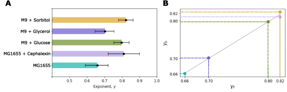
Figure 3. Estimation of scaling exponent using bootstrapped data for different growth conditions. (A) The mean gamma (colored bars, black circles) for the different growth media (M9 + sugar) and drug treatment are compared. Bootstrapping was performed by sampling over 103 bootstraps with sample size of N/5, where N is the population size. The error bars (black) represent the upper 97.5% and lower 2.5% quantile bounds. This represents the 95% confidence interval. (B) A scatter plot of γ obtained from bootstrapping (γb ) vs that obtained using the fit to the whole data set (γf ) shows strong correlation (ρ = 0.99). Colors: growth conditions, gray: straight line fit. Experimental data was taken from figures 1 and 2.
Download figure:
Standard image High-resolution imageExperimentally measured differences in cell length obtained by modulating the growth rate alter both the mean and the spread of the distribution, as seen for example in the case of cephalexin treatment. In order to distinguish which of these influences the change in the SA-V scaling exponent, we used statistical simulations, since we were unable to separate the two effects experimentally.
2.5. Simulating the effect of increasing mean cell size and variability on SA-V scaling
Controlling cell length mean and standard deviations independently in experiments is technically challenging, therefore we use statistical simulations to address whether variability or means of lengths affect the scaling exponent. With these simulations we aim to find the statistical relations between cell lengths and widths that will give rise to the scaling observed. For simplicity, they do not include any mechanism or relation between cells over successive divisions. To this end we have modeled two scenarios:
Model 1: Increasing mean length with constant variability (s.d.): Motivated by Schaechter's law and our own experiments, where increasing growth rate results in increased mean cell lengths, we examined mean cell lengths ranging from 1 to 12 µm. In order to test the effect of increasing the mean and a proportionate standard deviation, we simulated cell lengths by sampling a lognormal distribution with increasing means from 0.1 to 2.5 µm and constant standard deviations (table 1). The resulting output arithmetic mean length and width distributions are comparable to experimentally measured cell lengths (figure S1(A)). The widths were simulated by sampling from normal distributions with their means increasing proportionately, based on a constant aspect ratio, AR
of 4.5 (figure S1(B)). As a result, for longer cells, the width is effectively constant, since the spread of cell lengths is much greater than that of the corresponding widths. As discussed in the earlier sections, constant width results in high scaling exponent values ( –0.9). Therefore, as expected, we find that the γ value of short cells (mean length 1.13 µm) is ∼0.65, while for long cells (mean length 12.44 µm) it increases up to ∼0.93 (figure S1(C)), with output means and standard deviations described in table 1. Averaging of SA and V, that eliminates population variability, results in the recovery of the geometric scaling exponent of γ = 0.67 (figure S1(C) inset). This demonstrates that even though the mean length and width increased proportionately (constant aspect ratio), the population variability governs the scaling relation. Thus averaging, that eliminates the variability, and the SA-V scaling exponent reverts to 2/3. When we maintain the distribution data, the increasing mean also corresponds to an increase in the exponent (figure S1(D)).
Table 1. Parameters used in the statistical simulations. Simulations of cell size lengths used INPUT lognormal mean (LM) length ( ) and standard deviations (LS) (
 ) resulting in OUTPUT values that are arithmetic mean (AM)
  and s.d. (AS)
  . The values correspond to data plotted in figures 4 and S1. The range of values used in the simulations correspond to the two models tested: (i) increasing values of length for constant s.d. and (ii) a range of s.d. for a constant mean. The models are described in detail in section 4.
| INPUT | OUTPUT | ||
|---|---|---|---|

|

|

|

|
| (i) Model of increasing means, constant s.d. | |||
| 0.1 | 0.2 | 1.13 | 0.23 |
| 0.5 | 0.2 | 1.68 | 0.34 |
| 1 | 0.2 | 2.77 | 0.56 |
| 1.5 | 0.2 | 4.57 | 0.93 |
| 2.5 | 0.2 | 12.44 | 2.53 |
| (ii) Model of constant mean, increasing s.d. (Simulation 0) | |||
| 1 | 0.1 | 2.73 | 0.27 |
| 1 | 0.2 | 2.77 | 0.56 |
| 1 | 0.3 | 2.84 | 0.87 |
| 1 | 0.4 | 2.94 | 1.22 |
| 1 | 0.5 | 3.08 | 1.64 |
Model 2: Increasing variability (standard deviation) for constant mean length: In order to address whether the increase in γ seen in the earlier simulations can be attributed to spread alone, we simulated distributions with mean cell lengths between 2.73 and 3.05 µm and increasing standard deviation 0.27–1.64 µm, based on an input lognormal mean of 1 µm and lognormal s.d between 0.1 and 0.5 µm (figure 4(A)). While the distribution has a constant lognormal mean, the output arithmetic mean increases slightly from 2.73 to 3.08 µm, as a result of an increased s.d., a feature of the distribution. These changes are very small compared to those in Model 1. The corresponding mean widths calculated from the arithmetic mean length and constant aspect ratio (AR = 4.5), therefore also show a slight increase 0.61–0.68 µm. (figure 4(B)). We find the SA scales with V with the exponent increasing from γ of 0.72 to 0.89 (figure 4(C)). Once more averaging the SA and V data from the population to get just one average value of SA and V for each distribution, resulted in the geometric scaling exponent of 0.67 (figure 4(D)). When the mean changes very little and the s.d. is increasing, the coefficient of variation of length (CVL ), i.e. s.d./mean, is expected to increase. We find that this specific combination of the fixed mean and increasing s.d. results in an increase in the scaling exponent γ with CVL , that is qualitatively similar to experiment (figure 4(E)). We refer to this as Simulation 0. In order to match experimental data, we simulated the simultaneously varying the mean and standard deviation, that we refer to as Simulations 1, 2 and 3 (table S1 and figure 4(E)).

Figure 4. Simulating the effect of constant mean cell length and increasing variability on SA-V scaling. (A), (B) Cell size variability was simulated such that (A) cell-lengths follow a lognormal distribution with a constant mean and increasing s.d. (table 1), (B) while widths follow a normal distribution. (C) SA plotted as a function of V with each point representing a simulated cell sampled from the distributions, was fit to the scaling relation (equation (1)) to obtain the exponent γ. (D) A plot of average SA and V obtained for each distribution of lengths-widths is fit to equation (1) to estimate γ. (E) The γ values as a function of the coefficient of variation of the length (CVL
) are plotted comparing simulations (Sim0–3) with experiment (gray circles) (table 2). Sim0: simulations with a constant mean and increasing s.d. of length as described in (A) and table 1, Sim1, 2 and 3: both mean and s.d. of length are varied (table S1). Colors: cell length distributions, with their corresponding width distributions.  for each distribution.
Download figure:
Standard image High-resolution imageThis led to a more general question of how changing the mean and standard deviation of a lognormal distribution of lengths could affect γ. In order to address this, we simulated a range of cell length distributions with their means and s.d. systematically varied, while widths were calculated as before to maintain a constant aspect ratio of 4.5. The fit of the resulting SA-V to the power-law (equation (1)) showed that estimated values of γ are more sensitive to the s.d. as compared to the mean (figure 5(A)). Representative distributions of four samples from this phase-like diagram are used to demonstrate the differences (figures 5(B) and (C)).
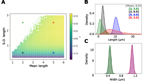
Figure 5. Simulating the effect of varying both mean cell length and variability on SA-V scaling. (A) Simulations were performed with increasing cell length mean and s.d. to generate lognormal distributions, with widths calculated based on a fixed aspect ratio of 4.5. The resulting SA with increasing V was fit to obtain a range of scaling exponents γ (color bar). White region: γ not estimated. The symbol 'x' marks representative points sampled in the phase-space with their respective (B) cell length and (C) width distributions plotted. Colors correspond to the mean and s.d. pairs from (A).
Download figure:
Standard image High-resolution imageBased on the results from experiment and simulation, variability appears to play an important role in estimating the exponent of SA-V scaling. Since experimental data was sampled from an unsynchronized population, we proceeded to test whether the statistics would still hold true for single cell data.
2.6. Single cell growth dynamics result in SA-V scaling by an exponent ∼0.9
We grew E. coli MG1655 expressing GFP on nutrient agar pads and imaged them in fluorescence (section 4). Cells were visualized by expressing the fluorescent protein GFP from a plasmid. We used a MATLAB based image-analysis pipeline to track representative cells from image time series (figure 6(A) and supplementary videos SV1(A)–(C)) to obtain length and width dynamics. Representative scatter plots of SA with V for each individual cell as a function of cell division progression, with time encoded in color, were fit by the scaling relation (equation (1)) and resulted in an exponent γ between 0.8 and 0.9 (figure 6(B)). Pooling multiple cells (n = 12) with the time course data obtained from tracking resulted in a fit exponent value of γ of 0.9 (figure 6(C)). When each individual cell time course of SA-V was fit, it resulted in a distribution of γ with a mean of 8.2 (figure 6(D)).
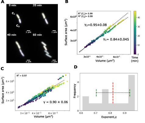
Figure 6. Effect of single cell growth dynamics on SA scaling with V. (A) Images of E. coli MG1655 expressing GFP from a plasmid grown on agarose pads show individual time-points from time-lapse microscopy. Time: min. Scale-bar: 1 µm. (B), (C) The SA was plotted as a function of V with time encoded in color (B) for two representative daughter cells C1 and C2 with scaling exponents γ of  and
and  respectively and (C) for 16 single-cell time series fit to one line resulting in
  . (D) Frequency histogram depicts the distribution of exponents obtained when each time-series was fit individually. Mean (red dashed line) and s.d. (green dashed lines) of the exponents are also represented.
Download figure:
Standard image High-resolution imageThus we demonstrate that the scaling exponent of SA-V obtained from time-course dynamics population sampled exponents both exceed the 2/3 value expected from the geometric law.
2.7. Effect of cell length variability dynamics during E. coli cell growth on SA-V scaling
In order examine whether the SA-V scaling exponent has any relation with cell division stages, we 'virtually synchronized' the single cell time-series data. The frame in which cells are born were noted as time zero and every frame number in the time series, fi
(i
 frame), is normalized by the doubling time resulting in a relative frame number
  , where fb
and fd
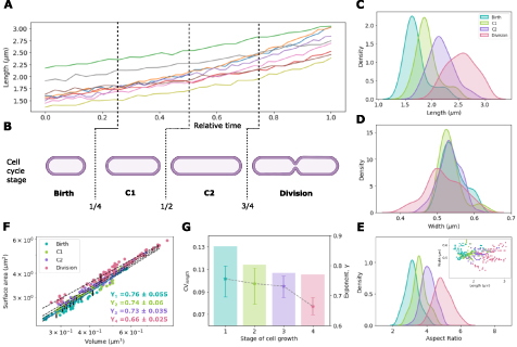
are the frames corresponding to cell birth and division respectively. We divide this relative frame number series into four equal parts that we refer to as B [0–0.25], C1 (0.25–0.5], C2 (0.5–075] and D (0.75–1], with the values indicating boundaries (figures 7(A) and (B)). This allows us to analyze the cell size distributions from length (figure 7(A)) and width dynamics as a function of stages. We estimate SA-V scaling from the single cell time-series of each stage. As expected, the mean of the cell length increases with 'stage' of cell division (figure 7(C)), while the width appears to have a constant mean but slight increase in spread (figure 7(D)). The resulting aspect ratio increases as the cell cycle progresses, a trend similar to that observed for the length (figure 7(E)). The length-width scatter shows poor correlation (figure 7(E) (inset)). SA-V scaling analysis for cell cycle stages results in exponents that change within the lifetime of cells (figure 7(F)). Surprisingly, we find the exponent γ and variability of lengths (CVL
) are the highest in B, and successively decrease in C1 and C2, and at division (D)
, where fb
and fd
are the frames corresponding to cell birth and division respectively. We divide this relative frame number series into four equal parts that we refer to as B [0–0.25], C1 (0.25–0.5], C2 (0.5–075] and D (0.75–1], with the values indicating boundaries (figures 7(A) and (B)). This allows us to analyze the cell size distributions from length (figure 7(A)) and width dynamics as a function of stages. We estimate SA-V scaling from the single cell time-series of each stage. As expected, the mean of the cell length increases with 'stage' of cell division (figure 7(C)), while the width appears to have a constant mean but slight increase in spread (figure 7(D)). The resulting aspect ratio increases as the cell cycle progresses, a trend similar to that observed for the length (figure 7(E)). The length-width scatter shows poor correlation (figure 7(E) (inset)). SA-V scaling analysis for cell cycle stages results in exponents that change within the lifetime of cells (figure 7(F)). Surprisingly, we find the exponent γ and variability of lengths (CVL
) are the highest in B, and successively decrease in C1 and C2, and at division (D)  , the geometric exponent (figure 7(G)). This suggests that cell size variability changes during the process of growth and division and is consistent with population statistics.
Figure 7. Effect of growth dynamics of single cells on variability and SA/V scaling. (A) The length (µm) as a function of relative time in the cell cycle is used to identify (B) four 'stages' of cell growth: birth, C1, C2 and division. (C), (D) The stage dependent frequency distribution of (C) cell lengths, (D) widths and (E) aspect ratio are plotted with inset: the corresponding scatter plot of individual lengths as a function of widths. The correlation coefficients (ρ) for length-width are 0.63 (Birth), 0.27 (C1), 0.19 (C2), 0.53 (Division). (F) SA is plotted as a function of V for individual cells. Each point represents an individual cell (n = 10). Colors represent the stage of the cell division cycle. The data was fit to the scaling relation to infer γ (±error based on 95% confidence interval). The R2 values for the fit lines to the stages Birth, C1, C2 and Division phases are 0.99, 0.97, 0.97 and 0.98 respectively. (G) The coefficient of variation of cell length, CVL
(bars) and estimated scaling exponent γ ( ) are plotted as a function of stage. Error bars in the γ are calculated by bootstrapping and represent the 95% confidence interval.
Download figure:
Standard image High-resolution image
3. Discussion
The scaling of SA and volume of cells is fundamental to comparative physiology and could offer insights into regulatory mechanisms at cellular scales. In this study we find that in populations of E. coli cell SA scales with volume with an exponent of  2/3 when cells are rapidly growing and sampled from mid-log phase. However, drug-induced filamentation or a range of sugars that modulate growth rate, result in higher exponents between 0.7 and 0.8, i.e. consistently higher than 2/3. Statistical simulations where either the mean cell length or the variability in cell length is systematically increased for distributions of cell lengths and widths result in SA-V scaling with an exponent greater than 2/3. Averaging the simulated SA and V distributions results in a return to the 2/3 scaling in simulations, demonstrating that population cell variability can alter the inference of the allometric scaling exponent of cell SA with volume. In order to test whether the lack of synchrony in populations had influenced our scaling exponent estimation, we measured SA-V scaling in growing single-cells and found
  0.7 to 0.9 during the life-span of a single cell, suggesting such scaling is intrinsic to E. coli growth and is independent of sampling. Finally we divided the cell division cycle into equal 1/4th parts and find cell length heterogeneity and by extension the geometric scaling exponent changes from ∼0.6 to ∼0.8, with the progression of the cell division stage. We find SA-V scaling exponent successively decreases from birth, through inter-division stage to dividing cells, that could have relevance for cell size control mechanisms.
In our experimental analysis, we have shown that the measured scaling exponent of SA-V scales with the growth rate of unsynchronized populations (figure 2(E)). In contrast simulated scaling exponents saturate with cell length variability (figure 4(E)). This could be explained by the fact that in simulations the cell shape as measured by the mean aspect ratio (length:width) is held constant. However, it appears that in experiment, cell length increase does not correspond to a proportionate change in cell width. This suggests that in order to obtain a better match of SA-V allometric relations between our model and experiments, we will need an improved model of cell shape regulation where a mechanical feedback between membrane curvature and envelope expansion maintain cell shape (Al-Mosleh et al 2022). An addition to such a model would be the reconciliation of population data of the kind presented here.
The functional and biological relevance of SA-V scaling, has been discussed previously in terms of its effect on the SA to volume ratio (SA/V), with suggestions that SA-V exponent exceeding 2/3 is beneficial for the uptake of resources (Huxley et al
1993, Okie 2013). We consider this for the rod-shaped geometry of cell populations with increasing sizes or higher variability, e.g. presence of filamentous cells. The area per unit volume (SA/V ratio) decreases with increasing size, based on geometry. Since nutrient uptake is required to cross the surface-barrier of a cell, the uptake rate per unit area, or flux, can be written as being proportional to area as  . By taking the product with 1/V on both sides we arrive at
  . Assuming V to be independently increasing, corresponding to larger cells, an increase in SA will be based on equation (2) and the SA-V scaling exponent γ. A γ value of 2/3 (or 0.66) will scale slower than 0.7 or 0.8, suggesting that flux will be higher for cells of the same length scale whose SA-V scale with
  . This could suggest a potential functional role for the observed exponents in E. coli cells.
In our calculations of cell length we have considered the pole-to-pole distance in the rod-shaped cell with  (equation (2)). This expression assumes that the hemispherical caps are projected onto a cylinder, based on previous work (Ojkic et al
2019). If we consider a hypothetical case of a very short cell, where the cell length would equal the sum of the radii of the two spheres, i.e.
(equation (2)). This expression assumes that the hemispherical caps are projected onto a cylinder, based on previous work (Ojkic et al
2019). If we consider a hypothetical case of a very short cell, where the cell length would equal the sum of the radii of the two spheres, i.e.  , where the radius itself is half the cell width
  . In such a case, the SA of the cell would be
  . The volume in turn would then be that of a sphere
  . In such a scenario the SA will scale with volume following the geometric law, i.e. with an exponent of 2/3. This is unaffected by whether the radius is normally distributed, based on our calculations. Such a scenario is unlikely to occur in our measurements since we ignore cells smaller than 1 µm in pole-to-pole length. At the same time it points to the importance of cell width regulation as an important factor in determining the scaling relation in rod-shaped bacterial cells.
Deviation of unicellular bacteria from the geometric 2/3 law is expected due to ecology and survival (Okie 2013). Indeed predictions of phenomenological models suggest cells may optimize their shape and size within the constraints governing the rate of SA addition relative to volume growth rate (Harris and Theriot 2016). However, a recent set of studies proposed gram-negative E. coli SA follows ideal geometric scaling with volume,  2/3, while for B. subtilis it is ∼0.83, that was interpreted as being indicative of alternative mechanisms at play in cell size growth regulation (Ojkic et al
2019). A growth rate model coupled to FtsZ assembly was developed to explain this difference in scaling (Ojkic and Banerjee 2021). In our data, we too find rapidly growing cells, potentially sampled in division phase, do scale with an exponent of 2/3. However, we find that irrespective of whether population cell sizes are sampled in rapid growth conditions or single cell growth dynamics are examined, the exponent is consistently higher than the geometric law. Our approach could be used to provide further inputs to disambiguate between multiple phenomenological models of bacterial cell size regulation such as 'sizer', 'timer' and 'adder'.
2/3, while for B. subtilis it is ∼0.83, that was interpreted as being indicative of alternative mechanisms at play in cell size growth regulation (Ojkic et al
2019). A growth rate model coupled to FtsZ assembly was developed to explain this difference in scaling (Ojkic and Banerjee 2021). In our data, we too find rapidly growing cells, potentially sampled in division phase, do scale with an exponent of 2/3. However, we find that irrespective of whether population cell sizes are sampled in rapid growth conditions or single cell growth dynamics are examined, the exponent is consistently higher than the geometric law. Our approach could be used to provide further inputs to disambiguate between multiple phenomenological models of bacterial cell size regulation such as 'sizer', 'timer' and 'adder'.
Our observation of a dependence of cell size variability and scaling exponent on the phase of the bacterial cell division cycle (figure 7(G)) could be the result of transcription, translation, replication, segregation or metabolic processes, either individually or in combination. Interestingly the transcription-translation 'noise' of genes has been shown to be dominated by translation strength and stochastic bursting of protein expression as observed in Bacillus and shown to be a general principle for prokaryotic gene expression (Ozbudak et al 2002). RNA levels themselves were found in E. coli to be increase and drop in the progression of one cell division cycle (Golding et al 2005). However, protein expression levels in single E. coli cells were seen to fluctuate with a period longer than the bacterial cell cycle with most of the noise 'extrinsic' (Taniguchi et al 2010). Growth rate fluctuations have been shown in a comparative study to probably be a major source for phenotypic variability contributing to deviations from the 'adder' model of cell size at division (Grilli et al 2018). In this regard a recent single-cell growth dynamics study has demonstrated that the instantaneous growth rate variance is high at birth and decreases as the cell approaches division, determined by nucleoid segregation dynamics (Gelber et al 2021). This could be the possible process driving progressive decrease in cell length variability and γ with cell cycle from birth to division, while widths remain largely unchanged. A synthesis of all the mechanistic sources for cell-division phase dependence of variability could help achieve an improved understanding of the molecular processes driving single bacterial cell division.
In conclusion, we find SA-V scaling exponents of single cells of E. coli to exceed the geometric exponent value of 2/3 in a manner that depends on drug-induced filamentation, varying growth rate and cell growth dynamics. Statistical simulations demonstrate that without the inclusion of population variability the SA-V scaling exponent reverts to the geometric law. We find, that the dynamics of single cell growth in multiple experiments, recapitulates the scaling exponent measured in population ensembles and provides quantitative data that can be compared to phenomenological and mechanistic models of bacterial cell division.
4. Materials and methods
4.1. Bacterial culture and sample preparation
Analysis of populations of cells sampled from mid-log involved growing E. coli MG1655 in multiple liquid media. Cells were grown in either (a) LB with and without 10 µg ml−1 cephalexin for filamentation or (b) M9-salts supplemented with different carbon sources to modulate the growth rate, with either (i) glucose (4% w/v), (ii) sorbitol (4% w/v) or (iii) glycerol (4% v/v) (Fisher Scientific, Mumbai). Growth rates were measured by monitoring optical density at 600 nm (OD600) every 10 min in a multiwell plate reader (Varioskan Flash2, Thermo Fisher Scientific, Waltham, MA, USA) and fitting the data to a logistic function, as described previously (Gangan and Athale 2017). At mid log-phase, cells were sampled, washed three times with 1% sterile phosphate-buffered saline (PBS) and mounted on slides coated with 10 µl of 1% (w/v) low-melt agarose (HiMedia, Mumbai, India) and observed in microscopy.
Single-cell growth dynamics was performed using E. coli MG1655 transformed using the Hanahan's method of CaCl2 chemical competence and heat shock (Sambrook and Russell 2001) with a GFP expression plasmid based on a pET15b backbone with a P hybrid promoter (AND-gate). Cells were grown overnight in LB at 37 ∘C, of which 10 µl spread on an
  cm2 agarose pad made on a slide using 1.5% Agarose in LB supplemented with 100 µM IPTG and 0.7% (w/v) arabinose. A coverslip with the agarose pad was placed on a custom-built 3D printed holder for time-lapse microscopy.
4.2. Microscopy
Single time point microscopy of populations: Cells grown in growth media were washed in PBS and a 5 µl droplet was placed on an agarose-pad and imaged in 100× (N.A. 1.45) phase contrast mode using an Olympus upright microscope with Olympus cellSense Dimension 3.1 software for image acquisition (Olympus Corp., Japan) and a CCD camera Hamamatsu ORCA-flash4.0 (Hamamatsu Photonics, Japan).
Time-lapse microscopy of single cells: Cells were mounted between two coverslips and imaged using a 100× N.A. 1.4 objective in fluorescence (excitation/emission 488/510 nm) for GFP mounted on a Nikon TiE inverted epifluorescence microscope illuminated with a 130W Intensilight Optic Illumination with control software NIS Elements ver.4.30.01 (Nikon Corp., Japan). Images were acquired on a CCD camera Andor Clara 2 (Andor, NI, U.K). Images were acquired at 1 min intervals for 60 min.
4.3. Image analysis
All low level image intensity adjustment, selection of regions of interest and adding scale-bars was performed using Fiji (Schindelin et al 2012).
In order to detect cell outlines, we developed an analysis pipeline in MATLAB (Mathworks Inc. Natick, MA, USA) using functions provided through the Image Processing Toolbox. The workflow was as follows: (a) cell outlines were identified by a combination of edge-detection by the Canny method (Canny 1986), gaps filling, and regions bridging. (b) Cells were filtered based on a minimum solidity criterion between 0.3 and 1 to remove small and irregular objects, with cell boundaries were optimized using an edge-based active contour method (Kass et al 1988), with a smoothing factor 1 and a contraction bias of −0.1. (c) Optimized contour boundaries were overlaid on the original input image and artifacts were interactively deselected to avoid cell debris and out-of-focus cells. (d) The remaining cells with contours were analyzed for length and width by first detecting the midline, and widths taken from averaging the 3rd and 4th quartiles of the minimal distance between the midlines and the contour boundaries. By taking only the top 50% values we exclude narrow widths at the ends of the cell from the analysis.
The code is available as OpenSource and can be downloaded from https://github.com/CyCelsLab/bacterialsizeScaling. The mean, standard deviation and the CV of the obtained lengths and widths is reported in table 2.
Table 2. Experimentally measured statistics of E. coli MG1655 cell sizes under multiple growth conditions. The mean ± standard deviation (s.d.) and median values cell lengths and widths measured in experiment are reported here. These correspond to the data plotted in figures 1 and 2. LB: lysogeny broth and M9: minimal medium.
| Growth condition/ media | Mean ± s.d. | Median | CV (σ/µ) |
|---|---|---|---|
| Length | |||
| LB | 3.15 ± 0.67 | 2.90 | 0.21 |
| LB + 10 µg ml−1 cephalexin | 6.34 ± 2.61 | 5.05 | 0.41 |
| M9 + 0.4% glucose | 6.00 ± 2.31 | 5.73 | 0.38 |
| M9 + 0.4% glycerol | 4.00 ± 1.15 | 3.63 | 0.28 |
| M9 + 0.4% sorbitol | 4.71 ± 2.14 | 4.22 | 0.45 |
| Width | |||
| LB | 1.05 ± 0.16 | 1.04 | 0.15 |
| LB + 10 µg ml−1 cephalexin | 1.04 ± 0.11 | 1.03 | 0.10 |
| M9 + 0.4% glucose | 0.77 ± 0.11 | 0.77 | 0.14 |
| M9 + 0.4% glycerol | 0.81 ± 0.12 | 0.83 | 0.14 |
| M9 + 0.4% sorbitol | 0.80 ± 0.10 | 0.79 | 0.12 |
This approach was used for both single time-point images in phase contrast as well as fluorescence images of E. coli expressing GFP with small changes in parameters for detection.
4.4. Data analysis
Bacterial growth rates in different media were estimated by fitting mean data obtained from triplicate measurements of optical density at 600 nm every 10 min for 3 h to a logistic model. Comparable to previous work, we assume the cell geometry to be a spherocylinder. This allows us to use the cell length and width to calculate the SA as:

while the volume (V) is given by:
where L is the pole-to-pole length and w the cell width. The scaling relation between SA and volume (V) was obtained by fitting the data to the scaling relation in equation (1). To test the validity of the fit obtained by linear regression in log–log space, we estimated the bounds of the 95% CI using function regplot (Seaborn, Python) with the bootstrapping parameter n = 1000. The shaded area around the data represents the CI. The aspect ratio (AR
) was calculated as  for each data point. In-house developed Python scripts were used to perform the calculations (Python3) using Pandas, NumPy, SciPy packages and Matplotlib (v3.4.2), with polyfit used for curve-fitting (Harris et al
2020).
for each data point. In-house developed Python scripts were used to perform the calculations (Python3) using Pandas, NumPy, SciPy packages and Matplotlib (v3.4.2), with polyfit used for curve-fitting (Harris et al
2020).
The CV was calculated as standard deviation/mean for the simulated distributions and length distributions from experiments.
Acknowledgments
We are grateful to Nishad Matange for the gift of E. coli MG1655 and to Sunish Radhakrishnan for access to phase-contrast microscopy. Aman Soni and Neha Khetan are acknowledged for discussions on data analysis. We are grateful to the anonymous reviewers for discussions that have helped improve this manuscript.
Data availability statement
The data that support the findings of this study are openly available at the following URL/DOI: https://github.com/CyCelsLab/bacterialsizeScaling/tree/image-analysis.
Funding
This work is supported by Grant BT/PR40262/BTIS/137/38/2022 from the Dept. of Biotechnology, Govt of India to C A A. T K is supported by a fellowship from IISER Pune. D K is supported by a fellowship from the Department of Biotechnology, Government of India (DBT/2018/IISER-P/1154).
Author contributions
Tanvi Kale wrote the code, performed the experiments and analyzed the data. Dhruv Khatri wrote the analysis code and optimized the analysis. Chaitanya Athale supervised the project, wrote the paper and obtained funding support.
Supplementary data (0.8 MB PDF) "The material contains additional figures and the description of the supporting movie file."
Supplementary data (0.2 MB AVI)
Supplementary data (0.1 MB AVI)
Supplementary data (0.1 MB AVI)