

Abstract
Most aggressive cancers are incurable due to their fast evolution of drug resistance. We model cancer growth and adaptive response in a simplified cell-based (CB) setting, assuming a genetic resistance to two chemotherapeutic drugs. We show that optimal administration protocols can steer cells resistance and turned it into a weakness for the disease. Our work extends the population-based model proposed by Orlando et al (2012 Phys. Biol.), in which a homogeneous population of cancer cells evolves according to a fitness landscape. The landscape models three types of trade-offs, differing on whether the cells are more, less, or equal effective when generalizing resistance to two drugs as opposed to specializing to a single one. The CB framework allows us to include genetic heterogeneity, spatial competition, and drugs diffusion, as well as realistic administration protocols. By calibrating our model on Orlando et al's assumptions, we show that dynamical protocols that alternate the two drugs minimize the cancer size at the end of (or at mid-points during) treatment. These results significantly differ from those obtained with the homogeneous model—suggesting static protocols under the pro-generalizing and neutral allocation trade-offs—highlighting the important role of spatial and genetic heterogeneities. Our work is the first attempt to search for optimal treatments in a CB setting, a step forward toward realistic clinical applications.
Export citation and abstract BibTeX RIS
1. Introduction
Cancer is a global healthcare problem that affects the lives of many people [1]. When oncologists deliver cytotoxic drugs to patients, cancer cells initially die, but unfortunately they quickly adapt achieving enough resistance to survive treatments [2]. Understanding the evolution of cancers and how to exploit it for an optimal treatment is an important open question [3] that could benefit from contributions of mathematics [4–8]. Population genetics provides a well-developed mathematical theory of evolution and its techniques have been applied to cancer [9]. On the other hand, control and optimization methods can be used to design treatment protocols that anticipate and even steer cancer evolution to patients' advantage [4, 6].
Mathematical models of cancer growth and evolution can be categorized according to how the population of cancer cells and its evolving phenotypes are described. Population-based (PB) models describe populations of identical cells [10–19] or sub-populations structured according to a discrete or continuous spatial variable [20–23]. On the other hand, individual-based (IB) models—cell-based (CB) in the context of cell populations [24–29]—describe each cell as an independent unit and can in principle incorporate any cell-specific and spatial heterogeneities [30–40]. The phenotype can be discrete, e.g., with two sub-populations of drug sensitive and resistant cells, or continuous, allowing degrees of resistance. Here we only refer to models that include adaptive resistance to a chemotherapeutic treatment. The list of references with the model basic features is summarized in table 1.
Table 1. References to PB and CB models of tumor growth and evolution that include adaptive resistance to anti-cancer treatment.
| References | Model type | Resistance phenotype | Time | Optimal strategy | Notes |
|---|---|---|---|---|---|
| [12] | PB | D | C | N | Survival prediction in patients with metastatic melanoma |
| [17] | PB | D | C | N | Analysis of the combined effects of chemotherapy and immunotherapy |
| [13] | PB | D | C | Y | Drug dosage maximization along with damage minimization in the treatment of bone marrow cancer |
| [14] | PB | D | C | Y | Optimal two-drug treatment of a cancer with sensitive and generalist/specialized chemoresistant cells |
| [16] | PB | D | C | Y | Maximization of the treatment duration, until a critical tumor size is reached |
| [19] | PB | D | C | Y | Minimization of the tumour volume, while preserving phenotypic heterogeneity |
| [22] | PB | C | C | N | Combined effects of cytotoxic and cytostatic drugs in a 2D-structured model of a vascularized tumor |
| [23] | PB | C | C | N | Continuous chemoresistance evolution in a 2D-structured model of a vascularized tumor |
| [20] | PB | C | C | N | Combined effects of cytotoxic and cytostatic drugs in a radial 3D model of a vascularized tumor |
| [10] | PB | C | C | Y | Optimal two-drug treatment under a continuous trade-off in the allocation of drug-specific resistance |
| [11] | PB | C | C | Y | Minimization of the tumor size at the end of treatment vs minimal average size during treatment |
| [15] | PB | C | C | Y | Minimization of the tumor size at the end of treatment; both tumoral and healthy cells are described |
| [18] | PB | C | C | Y | Minimization of a combination of tumor volume during treatment and drug side-effects |
| [21] | PB | C | C | Y | Extension of [20] that includes density-dependent drug and nutrients diffusion and rare mutations |
| [30] | CB | D | D | N | Modeling brain tumors that display clinically plausible survival times |
| [31] | CB | D | D | N | Combined effects of chemotherapy and 2-deoxy-glucose to control tumor size and chemoresistance |
| [33] | CB | D | D | N | Maximization of the time to tumor recurrence in a calibrated model on in-vitro experiments |
| [34] | CB | D | D | N | Analysis of the competition for space under therapy between healthy, cancer, and necrotic cells |
| [37] | CB | D | H | N | Analysis of the angiogenesis-induced resistance in brain tumors with two combined treatments |
| [38] | CB | D | H | N | Cell cycle dynamics in a vascularized tumor under chemo-radiotherapy |
| [39] | CB | D | H | N | Interplay among intracellular, extracellular, and intercellular factors in drug resistance |
| [40] | CB | D | H | N | Role of the spatial structure on the effectiveness of static and adaptive chemotherapies |
| [32] | CB | C | D | N | Combining effects of a chemotherapeutic agent and an epigenetic drug |
| [35] | CB | C | D | N | Emergence of drug tolerance under cytotoxic drugs administered at fix dosages |
| [36] | CB | C | H | N | Effects of metabolic heterogeneity on the growth of a vascularized tumor under different therapies |
PB models are typically continuous in time and amenable to mathematical analysis, such as optimal therapy control. They lack realism by assuming homogeneous (sub-)populations and therefore provide qualitative conclusions. Conversely, CB models are discrete in time or hybrid, e.g., with discrete cells generations and continuous fluid dynamics (H in table 1). Detailed CB models are so complex, typically designed in a stochastic framework, that they can be solved only through numerical simulation. They however have the potential to match in-vitro or clinical case studies and provide trustworthy predictions [24–26, 28, 38, 40].
All models mentioned in table 1 have been used to investigate the interplay between different control strategies in cancer chemotherapy and the cancer adaptive response to treatment. In all CB cases, different control strategies have been compared in terms of a target of interest, such as the tumor size at the end or during treatment, without facing the heavy computational challenge of an optimal control in the CB framework (no optimal strategy in table 1). Instead, in some PB cases, the search for the optimal strategy has been carried out ('Y' in table 1).
Among this latter group, an unstructured PB model proposed by Orlando et al [10] considers the interaction between two alternative cytotoxic drugs on a tumor that can adapt its drug-specific resistance. Despite its simplicity—the tumor is described as a single population of identical cells growing logistically—we find Orlando et al's model very interesting. It is the first attempt to model and optimally exploit an evolutionary trap for the tumor, known as evolutionary double bind [41].
The idea is to select the tumor for the specific resistance to one drug and then hit it with another one. This evolutionary scenario requires two decision variables, controlling the administration of the two drugs, and two phenotypes of the cancer cells that regulate the cell resistance specifically developed against the two drugs. Specifically, three types of drug-specific resistance allocation trade-offs are considered, differing on whether the cells are more, less, or equal effective when generalizing resistance to two drugs as opposed to specializing to a single one.
In this work, we extend Orlando et al's PB model to a CB setting, with the aim of testing, for the first time, an optimal control method on a CB model of cancer growth and evolution under treatment. We consider the choice of Orlando et al's model appropriate for two reasons. On one hand, the model is sufficiently complex to severely challenge optimal control in a CB setting—with two continuous phenotypes describing the overall and specific drug resistance and showing dynamical optimal protocols for one of the considered resistance allocation trade-offs. On the other hand, the model results are interesting and testing them beyond the homogeneous populations assumption make them more robust and transferable into practical clinical suggestions.
Nevertheless, our work intentionally makes only a preliminary step toward the optimal planning of clinical protocols. To design a computationally feasible test of optimal therapy control, we only exploit a few of the many modeling features allowed by the CB framework and only consider the basic control technique of gradient descent. Among the CB modeling features, the most important is the genetic heterogeneity of the cell population, that characterizes fast-evolving cancers [42, 43]. Indeed, the highly genetic heterogeneity of cancers is directly linked with drug resistance phenotypes [44].
We also include a 2D spatial structure, explicit competition for space, and the pharmacokinetics of drugs diffusion. We limit control to weekly drug dosages and monthly monitoring, a choice that limit the dimensionality of the optimization problem and that, at the same time, is closer to realistic clinical protocols. Although several CB models have been used in cancer modeling in the last years no one integrates all these aspects, in particular the search for the optimal treatment.
In the method section, we first summarize Orlando et al's PB model and results and then we present our CB model, its calibration, and our adaptation of the gradient descent control method. In sections 3 and 4, we present and discuss the obtained optimal control strategies. The main conclusion is that the knowledge of the type of trade-off in the allocation of drug-specific resistance—difficult to assess in clinical case studies—is not as crucial as suggested by Orlando et al's PB model. Independently of the type of trade-off, we find optimal protocols that exploit the evolutionary double bind [41], by inducing cancer cells to specialize to one drug and then hit them with the other one. Besides the trade-off-specific differences, we find that the optimal protocol obtained under the pro-specializing trade-off guarantees a significant gain, compared to static protocols, also when used under the pro-generalizing and neutral trade-offs. Conversely, the optimal protocols suggested by the homogeneous PB model are static under the pro-generalizing and neutral trade-offs. These substantial differences highlights the important role of spatial and genetic heterogeneities.
2. Methods
2.1. Background
Orlando et al [10] proposed a deterministic PB model to describe cancer growth and adaptive response to chemotherapy. The main equation is a simple logistic growth:
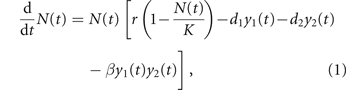
in which N(t) is the cancer size at time t (proportional to the number of cells) and y1(t) and y2(t) are the concentrations of the two administered drugs in the tumor body. In the absence of therapy, the tumor grows to a maximum size K (the so-called carrying capacity of the logistic growth), with exponential rate r at low size. The two drugs induce pharmacologic mortality of the tumor cell at per-capita rates d1 and d2 per-unit of drug concentration, respectively. Their joint action can cause an extra mortality (synergistic drugs, β > 0) or reduce their effectiveness (antagonistic drugs, β < 0); however, in the present work we only consider the case of non-interacting drugs (β = 0).
Since there is no spatial structure, the drug concentrations are assumed uniform throughout the tumor. Their clearance is modeled with first order pharmacokinetics

where z1 and z2 are per-unit drug clearance rates and w1(t) and w2(t) are the rates of drugs administration, i.e., the control variables at the disposal of the oncologist (drug mass per unit of time, assuming a unit dilution volume).
Cancer adaptive response to chemotherapy is described by a two-dimensional cell phenotype: one component, u ≥ 0, measuring the cell overall investment in drug resistance and one, u1 ∈ [0, 1], controlling the allocation of the acquired resistance to drugs 1 and 2. The larger is u, the larger is the fraction of the cell energy spent in the development and functioning of drug resistant mechanisms (u = 0 and u → ∞ corresponding to 0% and 100% of the energy, respectively); the smaller is consequently the cell energy spent in growth and duplication. The phenotype u therefore characterizes an energy allocation trade-off for the tumor between drug resistance and growth (see equation (3) below). Drug resistance can be fully specialized to one drug (u1 = 1 to drug 1; u1 = 0 to drug 2) or show any intermediate level of generalization toward both drugs. The resulting resistances to drugs 1 and 2 are defined by the products uu1 and uu2, where the allocation to drug 2, u2, is bound to u1 by one of the following drug resistance allocation trade-offs:
- (a)Neutral, implemented by the linear bound u2 = 1 − u1. It is the case of noninterfering drug resistances, in which the total resistance u(u1 + u2) equals the energy investment u.
- (b)Pro-specializing, implemented by the concave bound
 . It is the case of negatively interfering drug resistances, in which the total resistance is lower than the energy investment u (lowest if the cell maximally generalizes on both drugs at , see figure 1) and equals u only if the cell specializes on a single drug.
 - (c)Pro-generalizing, implemented by the convex bound. It is the case of positively interfering drug resistance, in which the total resistance is higher than the energy investment u (highest if the cell maximally generalizes on both drugs at , see figure 1) and equals u only if the cell specializes on a single drug.


The trade-off names refer to the fact that the interference between the allocated drug resistances favors, in terms of the total acquired resistance, cells that are specialized on a single drug or generalist. Since there is no individual structure, (u, u1) represents the mean phenotype of the population.
The tumor maximum size K and the mortality rates d1 and d2 are controlled by the phenotype in the following way. The maximum size is assumed to drop with the energy investment in drug resistance as a half-Gaussian bell

while the mortality rates decrease along with the specific drug resistance

where ki is the baseline level of resistance to drug i. These phenotypic-dependences define the energy allocation trade-off for the tumor between drug resistance and growth. The cell energy allocated to the biological processes conferring drug resistance is invested at the expense of energy otherwise allocated to cell growth and duplication. This reflects the real behaviour of many cancer cells that under chemotherapy slow down their cell cycle and develop drug resistance [45, 46].
The phenotype is assumed to be fully genetically determined (no epigenetic nor plastic responses are considered), with the two components controlled by non-interacting sets of genes. This allows to consider mutations acting independently on u and u1. The fitness of a mutation in evolutionary theory is the exponential rate of growth of the mutant population during its invasion transient [47, 48]. Denoting the mutant phenotype by (v, v1), the fitness is given by the per-capita growth rate of the mutant (v, v1)-population at low (technically zero) size, while invading the resident (u, u1)-population at size N:
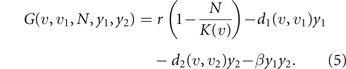
When the resident population is at equilibrium, its growth rate is vanishing, i.e., G(u, u1, N, y1, y2) = 0, so that the sign of the fitness, positive/negative, discriminates invading mutations from disadvantageous ones. For example, if treatment is interrupted after the development of some level of drug resistance u in the resident population, mutant cells with lower drug resistance have positive fitness (because of the higher maximum size K(v) > K(u), see equation (3), at y1 = y2 = 0), so that natural selection drives evolution toward the loss of the acquired drug resistance. In a deterministic setting, an invading mutation replaces the former resident type [49], so that the fitness gradient with respect to the mutant phenotype (v, v1) gives the direction of natural selection. Taking into account the stochastic nature of mutations, but looking at the limit in which they are extremely rare and each entailing an extremely small phenotypic change, the expected evolutionary dynamics of the mean phenotype is described by the following two equations:
(known as the canonical equations of adaptive dynamics [47, 48]), in which s is a time-scale parameter that goes to zero in the above limit. To describe real situations, s is taken proportional to the frequency of mutations and to the variance of the entailed phenotypic changes. The larger s, the lower is however the accuracy of equations (1)–(6) in describing the real demographic and evolutionary dynamics. When the frequency of mutations is of the order of one every few cell duplications, the paradigm underneath equation (6) of each invading mutant substituting the former resident type gets lost, as new mutations appears while the substitution transient is not yet over. In these situations a stochastic cell-based approach is more accurate.
Orlando et al's model of cancer growth and evolution under chemotherapy is composed of equations (1)–(6). The optimal control problem formulated in [10] finds the treatment (w1(t), w2(t)) in a given timespan [0, tf] that minimizes the final tumor size N(tf), starting from a fully grown untreated tumor

subject to the dynamics (1)–(6) and to the toxicological constraints

The optimal solutions under the three drug resistance allocation trade-offs (a)–(c) have a common beginning, during which both drugs are delivered at the maximum admissible rate to increase drug concentrations up to hit the toxicological constraints. Then, the solutions corresponding to the neutral and pro-generalizing trade-offs are constant and keep equal maximal drug concentrations for the rest of the treatment. Differently, under the pro-specializing trade-off, the optimal therapy is dynamic and alternates the two drugs. The therapy exploits the pro-specializing trade-off to select for tumor resistance for one drug and then hit the tumor with the other drug toward the end of the treatment.
2.2. Our cell-based evolutionary model
Unlike PB models, which are defined in terms of averaged per-capita demographic rates, cell-based (CB) models are IB. The model assumptions are made at the level of the single individual, the cell, about its characteristic parameters and about the procedural rules of interaction with the neighboring cells and with the surrounding environment. The population-level behaviour emerges bottom-up, as a result of the model simulation [50].
Though, in principle, any physiological and genetic detail can be included in a CB setting, we limit our description to a 2D spatial extension of Orlando et al's [10] PB model (described in the previous section). As discussed by Orlando and coauthors, the challenge for CB models of cancer growth, evolution, and treatment is computational, especially in the optimization of treatment. Our work is therefore to be considered a step forward to make the challenge feasible.
We represent space by a square grid of 100 × 100 nodes, with connection degree four, i.e., each node communicates with its four neighbors. Each node is a cell, which can be healthy or tumoral, though only the dynamics of the latter will be considered in line with Orlando et al's [10] model.
Each node is characterized by a state profile that includes the following information:
- The type of cell, healthy or tumoral.
- For tumor cells, the phenotypic strategy (u, u1): u ⩾ 0 is the overall energy investment in drug resistance; u1 ∈ [0, 1] is the resistance allocation to drug 1.
- The position of the cell in the grid, row r, top-to-bottom, and column c, left-to-right.
- The drug concentrations y1 and y2 at the location (r, c).
Time proceeds in discrete steps, each corresponding to an hour of real life. From a time step t to the next, the state of all nodes is updated according to the procedural rules described in the remaining part of this section. Some of the rules are stochastic, to better describe the intrinsic uncertainties of cellular processes, such as duplication, mutation, and death, and the regulating probabilities are scaled to the assumed time step. (An alternative, that we do not follow, is to stochastically draw the timing of the various events according to their rates of occurrence [51].)
2.2.1. Duplication
The cell cycle—cell growth up to cell division—of a cancer cell not investing energy in drug resistance (phenotype u = 0) is assumed to correspond to the time step. Although cancer cells often show cycles longer than 1 h [52], we consider a fast-growing tumor.
The energy allocation trade-off between growth and drug resistance is introduced by reducing the probability to complete the cell cycle in one time step along with the energy investment in resistance (phenotype u) [45, 46]. Specifically, we set the probability b(u) that the cell cycle is completed at the end of each time step (independently from one step to the next), by means of the following exponential relation:

where parameter b1 is calibrated (in section 2.3) to obtain an unviable tumor at a value of u at which the tumor maximum size K(u) of Orlando et al's model is negligible.
Note that the slope of function (9) at u = 0 is negative, in contrast to the zero slope of the maximum size K(u) in equation (3). This is a minor change, with respect to Orlando et al's model, that is however justified by energetic principles and will be quantified in section 2.3.
To introduce the inter-cellular competition for energy and space—described by the logistic growth in Orlando et al's model—the duplication of tumor cells (cell division) is assumed to occur at the completion of the cell cycle only in the presence of neighboring healthy cells. That is, we assume that the tumor grows by displacing healthy tissues.
Specifically, a neighboring location is randomly selected and duplication occurs only if the location is not occupied by another cancer cell. To minimize the spatial bias, cancer cells are considered for duplication in a new random order at each time step.
2.2.2. Mutation
Like Orlando et al's PB model, our CB extension describes the genetic of cancer at phenotypic level, and the two considered phenotypes are assumed to be fully genetically controlled by non-interacting sets of genes. Genetic mutations are therefore implemented as independent phenotypic variations at cell duplication, where only the daughter cell occupying the new location potentially mutates because of chromosomes copying errors.
The two phenotypes independently mutate with a probability μ. The extent of the mutation is drawn from a normal distribution with zero mean and standard deviation σ for the overall energy investment in drug resistance u and σ1 for the resistance allocation u1 to drug 1. If the resulting mutant phenotypes are unfeasible (u < 0 or u1 ∉ [0, 1]) they are forced to their extremal values. Parameters μ, σ, and σ1 are calibrated in section 2.3 to reflect the desired cancer evolutionary response.
Note that, because of the nonlinearity of the concave and convex bounds imposed by the pro-specializing and pro-generalizing allocation trade-offs (see cases 2 and 3 in section 2.1), mutations in u1 are not equivalent to opposite mutations in u2 (see figure 1). By implementing mutations on u1, the result is that symmetric scenarios, such as the administration of only one drug starting from zero resistance, do not yield symmetric model simulations. For example, after that cancer cells develop some resistance to drug 1 under the pro-specializing trade-off, a successful (positive) mutation of u1 (mutation at point A in the figure) corresponds to a smaller step (AB) on the concave trade-off curve, than the one produced by the opposite u1-mutation while administrating drug 2 at the symmetric point of the curve (step A'B').
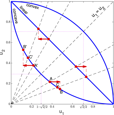
Figure 1. Drug resistance allocation. In Orlando et al's model, the interference between the two resistances is embedded in the phenotypes u1 and u2, i.e., point (u1, u2) lies on the trade-off curve (linear, concave, convex for the neutral, pro-specializing, pro-generalizing trade-off, respectively). We redefine the phenotypes as energy allocation fractions, so that point (u1, u2) lies on the linear curve u2 = 1 − u1. Taking the interference into account, the resulting resistances are given by the point (r1, r2) of the trade-off curve at the intersection with the ray through (u1, u2) (see points A, A' and C, C' before and after the mutations, shown for the pro-specializing trade-off). Mutations in u1 are equivalent to opposite mutations in u2 (both produce points C and C' in the two examples, whereas points B and B' are produced by the same mutations in Orlando et al's model).
Download figure:
Standard image High-resolution imageTo make mutations in u1 equivalent to opposite mutations in u2, we redefine the phenotype u1 as the fraction of the overall energy investment u in drug resistance allocated to drug 1, u2 = 1 − u1 being the fraction allocated to drug 2 (so that point (u1, u2) lies on the linear curve of figure 1, independently of the type of resistance allocation trade-off). Because of the interference between the two allocations, we assume that the amounts of energy actually available for effective drug resistant mechanisms against drugs 1 and 2 are given by the products ur1 and ur2, respectively, where r1 and r2 are the coordinates of the point of the trade-off curve sharing the same ratio u2/u1. That is, we look at the intersection of the trade-off curve with the ray passing through (u1, u2) (see figure 1). In formulas, we have
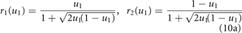
for the pro-specializing trade-off and
for the pro-generalizing one. Consequently, we redefine the pharmacologic mortality rates in (4) as

2.2.3. Mortality
We assume that the energy allocation trade-off also affects the cell death process. We therefore add to the pharmacologic mortality rates in (11) a natural mortality (not drug-induced)

that increases with the energy investment in resistance. Parameters b1 (in equation (9)) and m1 (here in equation (12)) measure the trade-off strength and are calibrated in section 2.3. In particular, m1 takes into account that the more energy is invested in drug resistance, the less remain for mechanisms resisting cellular death and avoiding immune destruction.
The total (per-cell) mortality rate during time step t is hence
where yi (t) is the concentration of drug i at the cell location. Because drug diffusion is simulated on a finer time scale with Ny sub-steps (see next section), the probability of cell death is evaluated at each sub-step k based on the drug concentrations yi (t + k/Ny ), k = 1, ..., Ny . Assuming an independent Poisson process for each cell within each time sub-step, each cancer cell independently dies in sub-step (t, k) with probability

2.2.4. Drugs diffusion
Being endowed with a 2D spatial structure, our model can describe the diffusion dynamics of the two considered drugs through the tissues represented by the cell-grid. We imagine that a capillary vessel is located in the grid top side, bringing oxygen and nutrients as well as the drugs. We assume that the drugs percolate top-to-bottom, following the pressure-gradient from the top artery region towards the bottom venous one, with no distinction between healthy and tumor cells.
Because the time scale of fluid diffusion through our body tissues is typically shorter than 1 h, we divide the time step into Ny equal sub-steps, t + k/Ny , k = 1, ..., Ny , and we update the drug concentrations yi (t + k/Ny ) accordingly, i = 1, 2. We also assume that the oncologist can directly control the drug concentrations wi (t) at the vessel in each time step (or, more typically, on a daily or weekly base), thus neglecting the vascular transport dynamics. Thanks to this simplification, the limitations imposed by the chemotherapeutic protocol on drug supply (see the constraints on w1 and w2 in (8)) imply that the constraints on the drug concentrations remain satisfied throughout the treatment.
The resulting diffusion dynamics, from sub-step (t, k) to sub-step (t, k + 1) is defined by the following equations:

r > 1, c ⩾ 1, where z is the fraction of the vascularizing blood that goes, every 60/Ny minutes, to the neighboring cell one row below. Left and right diffusion compensate, because we assume that the controlled concentrations wi (t) are homogeneously set in the grid top row (see equation (15a) for any column c). Parameter z is calibrated in section 2.3 to match the drug clearance rates of Orlando et al's model.
2.3. Model calibration
In the following subsections we present a series of simulations that we run to calibrate the parameters of our CB model to reflect the dynamical characteristics of Orlando et al's PB model. The involved parameters are listed in the subsection title. All model parameters and their values are summarized in table 2. The model has been implemented and numerically analyzed in the MATLAB environment.
Table 2. Summary of the model parameters and their calibration.
| Parameter | Value | Description |
|---|---|---|
| k1 | 10 | Baseline level of resistance to drug 1 |
| k2 | 10 | Baseline level of resistance to drug 2 |
| m0 | 0.1 | Non-pharmacological mortality |
| m1 | 1/210 | Energy allocation trade-off on death probability |
| b1 | 1/210 | Energy allocation trade-off on duplication probability |
| μ | 0.05 | Mutation probability |
| σ | 1 | Std. dev. of mutations in phenotype u |
| σ1 | 0.1 | Std. dev. of mutations in phenotype u1 |
| Ny | 25 | Number of time sub-steps for drug-diffusion |
| z | 0.75 | Drug clearance rate |
2.3.1. The demographic time scale (m0, k1, k2)
We use the same demographic time scale of Orlando et al's model. The exponential population growth rate r = 1 used in (1) implies that, at low density, the population doubles in about one time unit (log 2 is the doubling time at zero density). This is similar in our model, in which, at low density (low space competition), each cancer cell duplicates with high probability in one time step.
The use of similar time scales allows us to set the same rates of pharmacologic mortality, i.e., we fix k1 = k2 = 10 in (11), as done by Orlando and coauthors. Similarly, we fix the natural mortality rate m0 to 0.1, meaning that, with no drug resistance (u = 0 in (11)), a unit of drug concentration doubles the mortality rate of tumor cells.
2.3.2. The energy allocation trade-off (b1, m1)
To calibrate the energy allocation trade-off, we simulate the untreated growth of a non-adaptive tumor starting from four cells in the middle of our grid. We artificially test the unrealistic scenario in which a drug-free tumor is characterized by resistance u > 0 and we stop the simulation when the tumor is either extinct or reaches a stationary size. Extinction is unlikely at low u, whereas it certainly occurs if u is so high to excessively limit growth. Convergence to a stationary solution is obtained when the number of cancer cells, averaged over the last week, stays within a 1% variation for a week. The transition, for increasing u, from a positive tumoral regime to extinction corresponds to the exchange of stability between the two solutions (a bifurcation in the systems theory terminology).
The energy allocation trade-off between growth and drug resistance is controlled by parameters b1 and m1 in equations (9) and (12), respectively. We assume that the growth limitation equally splits between reduced cell duplication and increased mortality. We therefore set b1 = m1 and we search for the value that is consistent with the tumor maximum size of Orlando et al's model. Specifically, though the support of the Gaussian bell used in equation (3) is technically unbounded, most of the density occurs within three standard deviations, so that we look for the value of b1 yielding the above described extinction transition at about u = 90 ≈ 3σK (σK = 30 in Orlando et al's simulations). The result is obtained by averaging the regime tumor size over 10 simulations for each of a sequence of values of u. Figure 2 shows the result for b1 = 1/185.

Figure 2. Regime size (weekly-averaged cell number) of a cancer with homogeneous drug resistance u. Data are averaged over 10 simulations starting with four cells in the middle of the grid (positions (r, c) = (50–51, 50–51). Parameter values: k1 = k2 = 10, m0 = 0.1, b1 = m1 = 1/185.
Download figure:
Standard image High-resolution image2.3.3. Mutations (μ, σ, σ1)
The speed of the evolutionary process is controlled by both the frequency and size of the phenotypic mutations. We first calibrate the frequency, controlled by the probability μ that each of the two cell phenotypes mutates at duplication. We simulate a trait substitution transient to measure how long, on average, it takes for an advantageous mutation to spread and replace the outcompeted resident phenotype. We do this for the overall energy investment u in drug resistance. We randomly take a resident value in the viable interval of figure 2 and we run a simulation for each of the fully-grown tumors obtained to produce the figure. Each simulation starts from the fully-grown tumor, in which the drug resistance of a randomly selected cell is reduced by 10%, and the simulation continues until only one phenotype remains in the tumor mass. Because the grid is drug-free, cells with lower drug resistance are at advantage (because of the higher duplication probability in equation (9) and lower mortality in equation (12)) and typically invade and replace the resident type. This experiment is repeated for several values of the resident phenotype u and the average duration of the substitution transient turned out to be of the order of 1000 time steps.
To model a rapidly-evolving cancer, characterized by high phenotypic heterogeneity [43], we assume that about 50 mutations may occur, on average, during a substitution transient, so we set μ = 0.05. This choice is however rather arbitrary. It sets the separation between the demographic and evolutionary time scales. Taking into account that, on average, only half of the mutations are advantageous and that some advantageous ones get lost because of demographic stochasticity (accidental extinction and energy/space competition, especially on fully-grown tumors), the separation is about 1-to-100, i.e., one advantageous mutations per cell every 100 time steps (about 4 days).
Note that this separation is missing in Orlando et al's model, because the time-scale separation parameter s in equation (6) was not set sufficiently small (to reproduce their simulations, we had to use s = 4). The consequences of this oversight is that, on the timespan of the treatment (that lasts 8 time units in Orlando et al's simulations, see figure 3 in [10]), one also see the cancer growth dynamics and the pharmacokinetics of the drug concentrations. However, while the treatment typically takes months, cell demography and pharmacokinetics develop in hours, so that on the time scale of months the model should only track the equilibrium values of N(t), y1(t), and y2(t) corresponding to the current phenotypic status. Nonetheless, keeping the same ratio 1-to-100 introduced above, we interpret one time unit of Orlando et al's model as 100 time steps in our model.
We now turn to the calibration of the standard deviation σ of the mutations of the energy investment in drug resistance u. We focus on a five month two-drug static treatment (w1(t) = w2(t) = 5 at all time steps in equation (15a)) of a fully grown highly-adaptive cancer under the neutral resistance allocation trade-off. We look for the smallest value of σ for which, by the end of the treatment, the tumor fully develops drug resistance up to the level of energy investment u that balances the pros of reducing pharmacologic mortality with the cons of reduced growth (reduced duplication and increased natural mortality in equations (9) and (12)).
The simulation is repeated starting from the 10 fully-grown untreated tumors obtained without investment in drug-resistance (u = 0) to perform the experiments of figure 2. During the simulations, the developed drug resistance is equally allocated against the two administered drugs, i.e., the phenotype u1 is fixed at 0.5 for all cells with no mutations. This is an artificial scenario used only to the purpose of calibration. The convergence test for u is to have the last week average of the mean u in the tumor body within a 1% variation for a week. The resulting σ is slightly above 1.
Note that, in the same conditions, Orlando et al's model reaches the equilibrium value of the phenotype u in a much longer time (about 600 time units) than the 40 units corresponding to 6 months under the 1–100 unit-to-steps conversion set above. Indeed, the investment in resistance evolves quite slowly in Orlando et al's simulations (see again figure 3 in [10]), compared to the evolution of the resistance allocation u1 between the two drugs, that can reverts (from one drug to the other) in about 10 units (40 days). This is due to the use of the same scaling parameter s in front of the evolutionary equations in (6). As a consequence, the gain (in terms of tumor size) of the optimized treatment is quite limited in Orlando and coauthors' results (see discussion). This motivated us in considering a faster evolution of the energy investment in drug resistance.
Using σ = 1, we now calibrate the standard deviation σ1 of the mutations in the resistance allocation phenotype. Looking at the optimal treatment obtained by Orlando and coauthors under the pro-specializing allocation trade-off (see case 2 in section 2.1 and figure 3 in [10]), we see that in about 5 time units the tumor is able to evolutionarily specialize its resistance, from u1 = 0.5 to almost u1 = 1.
Taking into account the introduced time-scale relation, this means that, in our model, an evolutionary transient that completely reverts the allocation of resistance from one drug to the other should occur in about 1000 time steps. We therefore look for the value of σ1 for which the average u1 goes from 1 to nearly 0  in 10 forty-days drug-2 treatments (max dosage w2(t) = 10), under the pro-specializing allocation trade-off, starting from the 10 fully-grown untreated tumors obtained without energy investment in drug-resistance (u = 0) to perform the experiments of figure 2. The resulting σ1 is slightly below 0.1.
2.3.4. Drugs diffusion (Ny ,z)
The per-unit drug clearance rates z1 and z2 of equation (2) are equally set to 0.9 in Orlando et al's simulations. In the absence of drug supply, this yield a clearance period of about 5.5 units of time (five times the first-order time constant 1/0.9).
Considering the top-to-bottom diffusion described in section 2.2.4, we need more than 20 sub-steps (parameter Ny in equation (2)) to allow the drugs to percolate from the first to the last row of the grid in 5–6 time steps. We set Ny = 25 and found that z = 0.75 yields clearance (from yi,r,c = 1 in all locations to mean concentration below exp(−5) ≈ 0.0067, with no drug supply) in about 150 sub-steps.
2.4. Model testing
We test the calibration of our model by comparing the regime level of the energy investment in drug resistance u developed with constant maximum dosage of both drugs (w1(t) = w2(t) = 5 at all time steps) under the neutral resistance allocation trade-off (case 1 in section 2.1) against the level reached in Orlando et al's model.
With the parameter calibration of the previous sections (summarized in table 2, except for parameters b1 and m1 that were set at 1/185 in section 2.3.2), our model yields a regime value u ≈ 19, whereas u converges to about 22.5 in Orlando et al's model. To improve the matching, we slightly modify the parameters b1 and m1—respectively regulating the energy allocation trade-off between drug resistance and duplication and mortality—to the value reported in table 2, for which the tumor extinction shown in figure 2 occurs at about u = 100.
The result is shown in figure 3, averaged over 10 simulations starting from the same 10 fully-grown untreated tumors (initial phenotypes u = 0, u1 = 0.5) used in calibration (see sections 2.3.2 and 3). Convergence is obtained in about five months, consistently with the calibration of the mutation process (section 2.3.3). The solid black line is the average u (averaged over the grids of the 10 simulations at each time step); the shaded area indicates the standard deviation (computed over the 10 grids); the dashed line is the solution of Orlando et al's equations (1)–(6). Note that the time scale of convergence in Orlando et al's model (reported on the top time axis) is much longer than ours (one time unit of equations (1)–(6) corresponds to 100 time steps, about 4 days, in our model, so that the top time axis is rescaled to simultaneously show convergence). This is due to the missing separation, in Orlando et al's model, between the demographic and evolutionary time-scales (as already commented in section 2.3.3). However, by suitably rescaling time, the solution of Orlando et al's model (dashed line) is essentially within a standard deviation from the one of our calibrated model, indicating the agreement between the two models under a static chemotherapeutic protocol.
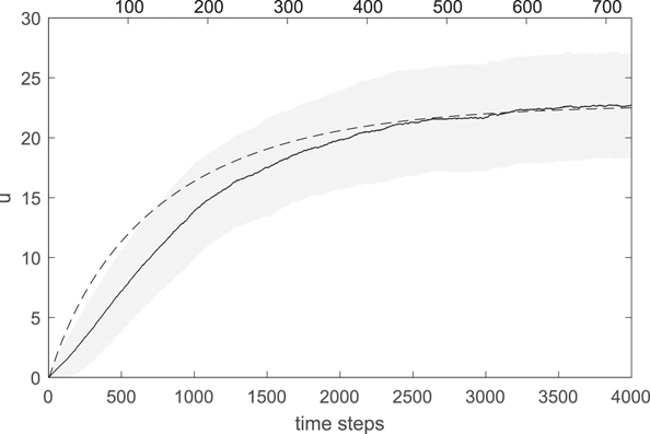
Figure 3. Evolution of the energy investment in drug resistance u under the neutral resistance allocation trade-off and constant protocol w1(t) = w2(t) = 5. Average and standard deviation (solid line and shaded area) computed over the grids of the 10 simulations starting from the fully-grown untreated tumors used in calibration (see sections 2.3.2 and 3). Parameter values as in table 2. The dashed line is the solution of Orlando et al's equations (1)–(6) (top time axis).
Download figure:
Standard image High-resolution image2.5. Control by gradient descent
To look for the optimal chemotherapy schedule, we assume that the drug supplies w1(t) and w2(t) are changed only weekly over a five-month period. Moreover, with no other toxicological constraint, the optimal solution necessarily lies on the bound w1(t) + w2(t) = 10 of maximum admissible dosage (equation (8)). The control variables are hence given by the 5 × 4 = 20 weekly dosages of drug 1, w1,k (w2,k = 10 − w1,k ), k = 1, ..., 20, that we pack in vector W. The control target is a functional of the cancer grow and evolutionary dynamics along the treatment, that we average over 10 realizations starting from the same fully-grown untreated tumors (initial phenotypes u = 0, u1 = 0.5) used in calibration (see sections 2.3.2 and 3). For example, to implement Orlando et al's target on the final tumor size, we look at the minimum number of cancer cell in the last week of treatment. Notwithstanding the intrinsic stochasticity, that we smooth out by averaging over 10 realizations, we qualitatively consider the target as a function F(W) of the control variables.
To minimize the target, we implement an adaptive version of the classical gradient descent method. Starting from a given control W(0) yielding target F(W(0)), the idea is to produce a sequence controls W(i), i ≥ 1, along which the target is reduced to a (possibly local) minimum. To find W(i) from W(i−1), we first perturb the control variables in W(i−1) one at a time by a fixed amount Δw (we use Δw = 0.5, i.e., 5% of the variable range; we use Δw = −0.5 if, when moving variable k,  ) and compute the kth component of the target gradient as
where E(k) is the kth vector of the canonical basis of the strategies space ( ; all other components being zero).
We then move the control variables in the direction

opposite to the gradient, by an amount ri that is the step size at the step i of the algorithm (variables that go out of range, w1,k < 0 or w1,k > 10 are truncated at 0 and 10, respectively). We first try the last step size, i.e., ri = ri−1 (r0 = 10). If we find a better control, i.e. F(W(i−1) + ri h(i)) < F(W(i−1)), the step is accepted, we set W(i) = W(i−1) + ri h(i), and ri is increased by 50% for the next step; otherwise the step size ri is halved and the target F(W(i−1) + ri h(i)) recomputed, until a better solution is found or the step size goes below a minimum threshold that we set at 10−5. If the minimum step size is reached, the gradient is recomputed at W(i−1) with halved perturbation Δw = 0.25 and the search is repeated starting with step size ri−1. If the minimum step size is again reached, the same is repeated with doubled Δw = 1, before the algorithm stops proposing W(i−1) as best solution.
To cope with the possible local minima, we always repeat the algorithm for each of three starting constant solutions W(0), the two single-drug protocols (w1,k = 10 and w1,k = 0 for all k) and the one that equally administers both drugs (w1,k = 5 for all k).
3. Results
3.1. Minimizing the cancer size at the end of treatment
In line with Orlando and colleagues [10], we look for the five-month chemotherapy schedule that minimizes the cancer cells number at some point during the final week of treatment. We note that with the calibration of the model parameters performed in section 2.3 and the dosage constraint w1(t) + w2(t) ≤ 10, the therapy is not able to eradicate the tumor, which persists even with the constant dosages w1(t) = w2(t) = 10 violating the constraint. Minimizing the tumor size at the end of a finite time horizon, could therefore be the optimal strategy before a removal surgery.
We find the same optimal weekly schedule, independently of the drug resistance allocation trade-off (neutral, pro-specializing, or pro-generalizing). The optimal solution exploits the evolutionary double bind mechanism [10, 41], administering only one drug but the final week, in which the other drug is used. This solution has a clear meaning. Giving only one drug during a time interval, the oncologist selects the cancer cells for a specialized resistance. This is true under any of the three resistance allocation trade-offs, because the pharmacologic mortality due to a single drug decreases by specializing the resistance along all the trade-off curves (see figure 1). At the beginning of the final week, the oncologist switches to the other drug and, after a washout period (which is rather fast, few hours, in our setting), cancer cells find themselves maximally sensitive to the new drug, while wasting the actual energy investment in drug resistance at the expense of reduced growth and survival rates. This is the worst scenario for the tumor, so that many cancer cells get killed and the tumor size rapidly drops.
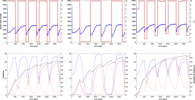
Because of the assumed rapid evolution of cancer cells, especially the rapid reallocation of drug-resistance (phenotype u1) resulting from the model calibration, once the new demographic regime is reached, the remaining cell start to revert the allocation, thus creating a more favorable environment for tumor regrowth. This is clearly visible in figure 4 (though the target in section 3.2 is different), when the drug concentrations are suddenly changed (red lines in the top panels). See, e.g., the middle panels under the pro-specializing trade-off: after a quick drop in about two days (blue in the top panel), the tumor size increases as long as the cancer cells reallocate their resistance to the new drug (blue in the bottom panel).
Figure 4. Cancer growth and evolution under the optimal five-month chemotherapy schedule with monthly monitoring mid-points. Left/middle/right: neutral/pro-specializing/pro-generalizing drug resistance allocation trade-off. Top: optimal schedule w1(t) (red on right vertical scale; w2(t) = 10 − w1(t)) and mean tumor size (blue on left vertical scale; averaged over 10 numerical realizations starting from the fully-grown untreated tumors used in calibration in sections 2.3.2 and 3). Bottom: phenotypes, averaged over the grids of the 10 realizations; overall and specific energy investments in drug resistance u, ur1(t), and ur2(t) (black, red-solid, and red-dashed, left vertical scale) and resistance allocation fraction u1 (blue; right vertical scale). Parameter values as in table 2.
Download figure:
Standard image High-resolution image
The minimum tumor size is reached at a specific time during the last week, to which the oncologist should carefully pay attention—possibly supported by tumour mass scanning—to optimally plan the removal surgery. The effective minimum, when it is achieved, and the obtained improvement with respect to the best and worst static protocols depend on the drug resistance allocation trade-off. Numerical results are reported in table 3.
Table 3. Targets numerically obtained under the three drug resistance allocation trade-offs and comparison with the best and worst static protocols (% of improvement provided by the optimal solution). Results are averaged over 10 realizations starting from the fully-grown untreated tumors used in calibration (see sections 2.3.2 and 3). Target: minimizing the number of cancer cells in the last week of the protocol (the final step is indicated counting from the beginning of the treatment). Best static protocol: both drugs at equal maximum dosage. Worst static protocol: only one drug at maximum dosage. Parameter values as in table 2. Computation performed on a CPU Intel Xeon(R) E5-2650@2.0 GHz.
| Res. alloc. trade-off | Best protocol mean (SD) | Final step (hrs) | CPU time (sec) | Best static mean (SD) | Final step (hrs) | Gain (%) | Worst static mean (SD) | Final step (hrs) | Gain (%) |
|---|---|---|---|---|---|---|---|---|---|
| Neutral | 1628.5 (63.96) | 3218 | 49 680 | 2851.6 (22.61) | 3360 | 48.15 | 4343.2 (72.25) | 3254 | 62.50 |
| Pro-specializing | 1230.9 (54.81) | 3233 | 38 780 | 2473.7 (45.30) | 3255 | 50.24 | 4272.9 (70.15) | 3207 | 71.19 |
| Pro-generalizing | 2139.0 (56.26) | 3210 | 67 272 | 3652.9 (73.34) | 3277 | 41.95 | 4414.2 (50.65) | 3343 | 51.54 |
3.2. Monthly monitoring mid-points during treatment
We now imagine that the oncologist wants to keep the tumor mass under control along the treatment, e.g., with monthly monitoring mid-points. To this purpose, we minimize the averaged number of cancer cells during the last weeks of the five months of the protocol.
We discover that the optimal schedule is dynamic for all the investigated drug resistance allocation trade-offs (neutral, pro-specializing, or pro-generalizing). The three optimal solutions (numerically obtained and averaged over 10 realizations starting from the fully-grown untreated tumors used in calibration in sections 2.3.2 and 3) are displayed in figure 4 and share a common beginning: after inducing cancer cells to specialize by administering only one drug for three weeks (drug 1 in the figure), the other drug (drug 2), to which the tumor is at that point highly sensitive, is used during the first monitoring week to kill an effective number of cancer cells. Also note the significant initial drop of about 70% of the tumor size, from the untreated regime of about 8600 cells, due to the pharmacologic mortality. This drop is very fast (one-two days) also because of the quick pharmacokinetics (clearance in few hours).
Under the pro-specializing trade-off (figure 4 middle panels), cancer cells are not able to revert the allocation of resistance from drug 1 to drug 2 during the first monitoring week. Not even the generalized resistance at u1 = 0.5 is reached. Thus, in the first week of the incoming month, the drug used in the monitoring week is still the most effective. Moreover, while steering the tumor to exchange its specialized resistance from drug 1 to drug 2, the two actual allocations r1(t) and r2(t) must follow the concave trade-off curve of figure 1, along which the total resistance is lower than a fully specialized one and minimal at the point of generalized resistance u1 = 0.5. For both these reasons, after the monitoring week, the optimal schedule continues to administer the same drug also in the incoming month, up to the next monitoring week. At the beginning of the next monitoring week, the situation is the same as the previous month but with the allocation of resistance and drug concentrations exchanged. The oncologist can again exploit the evolutionary double bind mechanism [10, 41], hitting the cancer with the effective drug, and so on for the rest of the protocol.
Under the pro-generalizing trade-off, after the first three common weeks, to optimally exploit the evolutionary trade-off, the cancer cells must be hit with a mix of the two drugs (see figure 4, right, where w1(t) is nonzero in the fourth week). This is essentially due to the different speeds of evolution of the resistance allocation phenotype u1 toward specialized and generalized resistance. The first is smaller than the second, because of the shape of the convex trade-off curve (see figure 1, convex curve, where mutations close to specialized resistance to drug i yield minor changes in the actual allocation ri (t), whereas large changes occur in both r1(t) and r2(t) close to generalized resistance); the situation being reversed under the pro-specializing trade-off. Thus, at the beginning of the first monitoring week, the tumor is not fully specialized to drug 1, and this makes it easier to reach and pass generalized resistance u1 = 0.5 during the week. Moreover, evolution toward generalized resistance is sped up by the evolutionary trade-off, so that using only drug 2 would lead to a strong specialization to drug 2 and to a tumor regrowth that would increase our target function. The optimal drug mix turns out to allow the tumor to pass generalized resistance, so that it is convenient to switch back to drug 1 in the incoming second month. In the first week the tumor is indeed more sensitive to drug 1, though eventually the target requires to specialize the tumor to drug 1, to be again severely attacked by drug 2 during the second monitoring week. The control strategy is repeated in the following months, though the drug mix used in the monitoring weeks changes according to the evolution of the energy investment in resistance u (black line in figure 4, right-bottom), which modulates the speed of evolution of the resistance allocation u1.
Under the neutral trade-off (figure 4, left column), the optimal schedule found by our algorithm follows the same logic of the solution found for the pro-generalizing trade-off (right column). That is, the logic of using one drug to induce tumor specialization during the three consecutive unmonitored weeks and of hitting the tumor with the other drug during the monitoring weeks. The difference is that only one drug is used in the monitoring weeks (drug 2 in the figure), instead of a mix as it occurs under the pro-generalizing trade-off. The reason is again the relative speeds of evolution of the resistance allocation phenotype u1 toward specialized and generalized resistance. Indeed, under the neutral trade-off and compared to the pro-generalizing one, cancer cells evolve faster/slower toward specialized/generalized resistance, so that the tumor turns out to be more specialized at the beginning of a monitoring week and can be hit with the effective drug at maximum dosage (drug 2) without inducing excessive tumor specialization and regrowth. During the monitoring week, the allocation phenotype u1 crosses generalized resistance u1 = 0.5, so that the best strategy is to switch back to the first administered drug (drug 1) to induce tumor specialization in the new incoming month.
We note that, under the neutral trade-off, the optimal schedule we found for the pro-specializing trade-off is equally optimal (differences are within the variability due to the model stochasticity). Indeed, the neutral one is an intermediate case between the pro-specializing and pro-generalizing trade-offs. Table 4 reports the obtained target values (average tumor size in the monitoring weeks; results averaged over 10 realizations). Because the identification of the type of drug resistance allocation trade-off could be a critical issue for the oncologist, we apply the three identified best protocols to all cases. Interestingly, the target loss of using the best schedule for the wrong trade-off is limited and, in any case, smaller than the loss of using the best static protocol.
Table 4. Targets numerically obtained under the three drug resistance allocation trade-offs and comparison with the best and worst static protocols (% of improvement provided by the optimal solution). Each optimal protocol (n-, ps-, pg-best) is tested on the three types of trade-off to show the loss of using the wrong solution. The best solutions therefore lies on the diagonal of columns 2–4. Results are averaged over 10 realizations starting from the fully-grown untreated tumors used in calibration (see sections 2.3.2 and 3). Target: Minimizing the average tumor size during the last week of each month. Best static protocol: both drugs at equal maximum dosage. Worst static protocol: only one drug at maximum dosage. Parameter values as in table 2. Computation performed on a CPU Intel Xeon(R) E5-2650@2.0 GHz.
| Res. alloc. trade-off | n-best protocol mean (SD) | ps-best protocol mean (SD) | pg-best protocol mean (SD) | CPU time (sec) | Best static mean (SD) | Gain (%) | Worst static mean (SD) | Gain (%) |
|---|---|---|---|---|---|---|---|---|
| Neutral | 2452.8 (23.66) | 2458.9 (27.34) | 2471.8 (19.31) | 313 989 | 2935.5 (8.65) | 16.43 | 4012.4 (10.22) | 38.87 |
| Pro-specializing | 1976.3 (16.75) | 1960.8 (33.04) | 2102.8 (12.36) | 657 133 | 2507.1 (7.92) | 21.79 | 4101.8 (20.41) | 52.20 |
| Pro-generalizing | 3332.2 (17.81) | 3299.4 (18.68) | 3275.3 (15.93) | 610 607 | 3627.9 (11.48) | 9.72 | 4266.8 (10.41) | 23.24 |
Also note the significantly increased computational time with respect to table 3. The reason is that we incrementally optimized one more month of treatment at a time, starting from the obtained solution for the already optimized months and from the three constant solutions (the two single-drug and the one that equally administers both drugs) for the new month.
4. Discussion
We explored the in-silico optimal two-drugs chemotherapy schedule in a five-month treatment of an aggressive tumor showing a genetically-based drug-resistance evolutionary response. To this aim, we extended the PB deterministic model proposed by Orlando et al [10] to a more realistic cell-based (CB) stochastic framework. From a technical point of view, the challenge is computational, as the target to be optimized needs to be averaged over multiple realizations (simulations) of a three-time-scale demographic-evolutionary-clinical stochastic process. To the best of our knowledge, optimal control techniques have been so far applied only to PB models (see table 1), but we believe that it is time to go beyond this limit and explore optimal solutions using realistic CB models. We are now technically ready for this challenge, which has the potential to bring in-silico simulations closer to in vitro or in vivo clinical cases and provide support to personalized medicine.
We tackled the computational challenge by designing a first feasibility test. For this reason, we selected a relatively simple—yet interesting—deterministic PB model and we extended it to a CB stochastic framework by adding only few of the possible elements of realism allowed by the framework. We included only the elements we consider most relevant for describing cancer growth and evolution, that are the cell genetic heterogeneity (described at phenotypic level) that characterize fast-evolving organisms [42, 43], a 2D spatial structure, explicit competition for space, and drug diffusion following the artery-to-venous pressure-gradient. We also tested one basic optimization algorithm based on gradient descent. Computing the gradient of the desired target with respect to the many control parameters defining the drug-administration profile during treatment is the most costly and unreliable step. Although gradient-free methods are available, we think that the gradient computation and accuracy must be tested, before considering the exploration of other control techniques in future research. To limit the computational burden, we limited control to weekly drug dosages and monthly monitoring, a choice that is in any case closer to realistic clinical protocols.
Despite its simplicity, our model incorporates several of the ten worldwide recognized cancer hallmarks [53]: replicative immortality (each cell can potentially duplicate infinite times), genome instability (high mutation rate), evasion of growth-suppressor signals (each cancer cell always complete its cell cycle, duplication being limited only by energy and space), sustained proliferation (only space is limiting growth), resist cellular death and avoid immune destruction (small non-pharmacological mortality), altered metabolism (high energy/nutrients competition, indirectly modeled by space competition), tumor-promoting inflammation (not modeled), angiogenesis (indirectly modeled, as oxygen and nutrients reach all cells), and activation of invasion and metastasize (not modeled since we suppose that the tumor is fully grown in stage T3N0M0—using the globally recognised TNM classification of malignant tumors [54]—at the beginning of treatment).
In the CB framework, our model is the first to consider the demographic (cell cycle), evolutionary (phenotypic mutations), and clinical (treatment) time scales for a tumor endowed with two continuous phenotypes regulating the overall energy investment and specificity of the developed drug resistance. Following the assumptions of Orlando and colleagues [10], we investigated three different evolutionary trade-offs faced by the cancer cells in the allocation of resistance to the two administered drugs. In the neutral trade-off—the simplest assumption—there is no interference between the mechanisms of resistance to drugs 1 and 2, so that the developed resistance is split between the two drugs according to a splitting ratio that is assumed to be an heritable phenotype. In the pro-specializing and pro-generalizing trade-offs, the interference is respectively negative—the actual resistances are reduced by a factor that is largest when the cell is generalist, i.e., when the cell genotype is set for a 50% splitting (see figure 1 concave curve)—and positive—the actual resistances are amplified by a factor that is largest when the cell is generalist (see figure 1 convex curve).
The drug resistance allocation trade-off allows the oncologist to exploit the tumor evolutionary response to treatment. The underlying paradigm is that the oncologist plays rationally and can think ahead, solving an in-silico control problem to design an optimal strategy to be eventually applied in-vivo. Cancer cells instead follow only their evolutionary boost pushed by microenvironmental pressures and are selected if they spread at the expense of other outcompeted genotypes. This dynamic is distinctive of a leader–follower game [10, 55], where the leader chooses first the best strategy and the follower adapts. This is why adaptive drug resistance, that is considered one of the main strengths of cancers, can be transformed into a weakness, that can be anticipated, controlled, and even steered by the oncologists.
4.1. Optimal protocols and resistance allocation trade-offs
If the oncologist's goal is to reduce the tumor mass as much as possible in a prefixed time horizon, for example to schedule a removal surgery, the optimal protocol is the same independently of the drug resistance allocation trade-off. As exposed in section 3.1, the optimal protocol is to steer cancer cells to a specialized resistance by administering only one drug and then hit the tumor mass with the other drug, to which cancer cells are maximally sensitive. During this second phase, cancer cells suffer the highest mortality, but the surviving ones reallocate their resistance to the new drug and the mass eventually starts to regrowth. The tumor mass hence reaches a minimum to which the oncologist must pay careful attention.
Note that, when only one drug is administered, cancer cells specialize for that drug, even under the pro-generalizing resistance allocation trade-off. Moving along the trade-off curve (see figure 1) toward specialization to drug i, the resistance to drug i increases toward 1, so that the pharmacologic mortality induced by drug i monotonically decreases, i = 1 or 2. Once full specialization is reached, cancer cells are in the most favorable condition for the given drug dosage. Administering a single drug at constant maximum dosage is therefore the worst protocol among the ones using maximum admissible drug dosage.
Conversely, the best constant protocol is the one that equally administers both drugs at maximum total dosage. Under the neutral resistance allocation trade-off this is easy to see. Imagine a sequence of different constant protocols obtained from the worst one administering only drug 1 by replacing an increasing amount of drug 1 with the same amount of drug 2. The tumor cells optimal allocation of drug resistance then moves from fully specialized to generalist, while the resulting mortality rate increases along the sequence (see equation (13)). Because of the symmetry between drugs 1 and 2, the maximum mortality that can be achieved with a static protocol is hence the one obtained by administering equal constant amounts. Interestingly, the 'bang-bang' control—solutions in which only one drug is administered at a time—optimally exploits the evolutionary double bind mechanism [10, 41] and outcompetes the best static protocol by 40%–50% (detailed results in table 3).
Regarding the target with monthly monitoring mid-points (section 3.2), depending on the drug resistance allocation trade-off, we found two different logics of control. One makes mainly use of one drug, during the first three unmonitored weeks of each month to induce cells specialization, and administers the other drug in the monitoring weeks to severely reduce the tumor mass; the other is a bang-bang solution that alternates the two drugs, with the switch at the beginning of each monitoring week. The latter is optimal under the pro-specializing trade-off, whereas a version of the former that slightly mix the two drugs in the monitoring weeks is optimal under the pro-generalizing trade-off. For the neutral trade-off, the two bang-bang versions of the two solutions are equally optimal.
What makes one of the two logics optimal has to do with the relative speeds of evolution of the resistance allocation phenotype toward specialized and generalized resistance. Under the pro-specializing trade-off, cancer cells evolve faster/slower toward specialized/generalized resistance, whereas the situation is reversed under the pro-generalizing trade-off. In the first case, cancer cells are not able to specialize to the new drug during the monitoring week, because to do so they have to first evolve to generalized resistance. Consequently, they are still more sensitive to the new drug at the beginning of the new month. Moreover, by inducing full specialization to the new drug during the first three weeks of the new month, the optimal treatment also exploits the higher evolutionary cost, with respect to the pro-generalizing trade-off, of evolving along the concave trade-off curve (see figure 1).
Conversely, the tumor crosses generalized resistance and specializes to the new drug during the monitoring weeks under the pro-generalizing trade-off, also because the starting point at the beginning of the week is less specialized than under the pro-specializing trade-off, because of the slower evolution toward specialization. Actually, using only the new drug would induce a too strong specialization and a consequent tumor regrowth, so that the new drug is optimally mixed with the previous one used to specialize the tumor.
In clinical situations, the type of drug resistance allocation trade-off is most of the times unclear, if not unknown. On the one hand, our model suggests a way to estimate the trade-off curve. For example, a long-term experiment could monitor the reallocation of resistance from drug 1 to drug 2. First only drug 1 is administered to induce a fully specialized resistance, then only drug 2 is given to drive the reallocation. During this transient, the pharmacological mortality to drug 2 is monitored, and the one to drug 1 could be estimated on short experiments in which some cells are removed and treated with drug 1. From the pharmacological mortalities, a measure of the relative drug resistance could be inferred by a model like equation (4).
On the other hand, our results show that the bang-bang dynamic solutions identified by the two logics of control both achieve significantly better targets than the best static solution (see table 4, where n-best is the best protocol for the neutral trade-off, i.e., the bang-bang solution that makes mainly use of one drug, while ps-best is the best protocol for the pro-specializing trade-off, i.e., the bang-bang solution that alternates the two drugs). Under the uncertainty on the type of trade-off, the best protocol for the pro-specializing trade-off (ps-best in table 4) is preferable, because it is equally optimal for the neutral trade-off and quasi-optimal for the pro-generalizing one.
4.2. Comparison with Orlando et al's model
Confronting our results relative to the target at the end of treatment (section 3.1) against those obtained by Orlando and colleagues [10], we find a qualitative agreement only under the pro-specializing trade-off of drug resistance allocation. Both optimal solutions—our own and the one of Orlando et al's PB model—are dynamic and exploit the tumor evolutionary double bind. Besides the fact that the control variables—the drug dosages—are continuous in Orlando et al's model and discrete on a weekly base in our model, the solution logic is qualitatively the same: induce tumor specialization under the effect of a single drug and finally hit it with the other one.
Quantitatively speaking, however, there are significant differences. In the PB model, tumor cells are all identical, so they all homogeneously specialize under the effect of a single drug and they all suffer the highest mortality when the oncologist switches to the other drug. In the CB setting, the stochasticity of mutations, as well as that of demographic processes, always leaves some unspecialized cell that are immediately drug resistant when facing the new drug. In a way, the more realistic setting confers the tumor a more reactive adaptive resistance. This makes our solution sharper (bang-bang solutions) than the continuous oscillations obtained in the PB model. Moreover, our optimal strategy makes use of a single drug throughout the treatment, but the last period (the last week), to induce the highest specialization of the tumor cells. Conversely, the fact that full specialization is more easily reached in the PB setting makes possible to exploit the evolutionary double bind several times during treatment, though this option seems an artefact of the unrealistic setting. Without considering the toxicological or clinical constraints of administering one drug for a relatively long period, the best strategy to target the tumor size at the end of treatment is to exploit the evolutionary double bind trap only in the last phase of the cure.
Moreover, Orlando and colleagues focus on a very short treatment. Because they do not clearly set the time-scale separation between the demographic and evolutionary processes (see the comment in section 2.3.3 on the calibration of the mutation process), their unit of evolutionary time turns out to be equivalent to about 4 days in our simulations, so that the eight-unit span of their simulations must be confronted to a month in ours. Moreover, by setting the evolutionary rates (mutation probability and standard deviation of the phenotypic mutational step) to reach a regime of the average cells investment in drug resistance in about five months, we end up with a more aggressive (fast-adaptive) tumor than Orlando and colleagues. Indeed, the cells investment in drug resistance (phenotype u) reaches values of about 10 in one month in the optimal solutions in figure 4, whereas it nearly reaches 1 in Orlando et al's optimal solution under the pro-specializing trade-off (see the middle-right panel in figure 3 in [10]). With such a small resistance to allocate, the gain offered by the evolutionary trap is very limited. The target gain (tumor size at the end of treatment) with respect to the best static protocol is negligible (and not published in [10]), whereas the gain against the worst static protocol that administer only one drug is small (7.81%).
Under the neutral and pro-generalizing resistance allocation trade-offs, Orlando and colleagues find the best static protocol to be optimal, with limited gain against the worst protocol (4.92% and 14.6%, respectively). This is again due to the little resistance developed on the short cure horizon. Static and dynamic solution are practically equally effective in that context, having the cancer little resistance to allocate. Conversely, the explicit spatial and genetic heterogeneities of our model show that it is possible to take significant advantage of the neutral and pro-generalizing resistance allocation trade-offs, as well, using the same dynamical solution designed for the pro-specializing trade-off.
4.3. Future research directions
Our relatively simple test of applying optimal control techniques to a CB model of cancer growth and evolution can be extended in many directions. The challenge is to increase the model realism, in line with the recent advancements in cancer modeling [37, 38, 40] possibly tailoring to specific cancers and to personalized medicine, while keeping feasible the computational burden of control.
For example, cell metabolic processes and oxygen/nutrients transport could be explicitly modeled, together with mechanisms of angiogenesis, invasion of new tissues, and metastasis [36, 37]. Tumor geometry could be described with heterogeneous 3D structures, taking explicit account for the tumor micro-environment and for the location of the tumor in the human body [56].
As for the mechanisms of drug resistance, phenotipic plasticity could take into account the resistance developed by the cell in response to changes in its environment, such as the administration of a new drug. Especially the fast reallocation of specific resistance to drugs could be better described as a plastic [57, 58] or epigenetic [59, 60] response, rather than by permanent DNA modifications. Multi-drug resistance could also be added, letting mechanisms that are specific to a drug to partially give resistance to other drugs as well [61].
More realism could be achieved also on the clinical side. Longer time horizon could be considered, with more realistic clinical constraints, such as concentrated drug administration in day-hospital, rather than distributed over the week, and break periods in case of adverse circumstances.
More realism or specificity could be also introduced on the target of control. Multiple targets could be mixed in the objective function to be optimized, or some could be expressed in terms of solution constraints. For example, following the recent modeling literature on cancer, enforcing a static tumor volume while controlling time to tumor regrowth or phenotypic heterogeneity seem to be important targets, rather than tumor size [40, 42, 55].
On the side of the control method, gradient descend could be jointly used together with gradient-free exploration methods, such as those based on genetic algorithms, to avoid the costly computation of gradients at each step and, at the same time, allow a more global exploration of the control space.
Envisaging the eventual application in-vivo of our results, especially in the context of personalized medicine, ideas from model predictive control could be incorporated to close the loop with the patient. The idea is to plan the optimal cure on a calibrated model initialized on the measured patient's state, apply the cure on a relatively short time horizon, and then replan it from the actual state reached by the patient.
Finally, modeling advancements should also be accompanied with experimental ones, and modeling could actually suggest experimental directions. For example, the two-drug resistance allocation trade-off introduced by Orlando and colleagues [10] and reviewed here (see section 2.2.2) seems to play a role in determining the optimal cure, so that its experimental identification is interesting (as discussed in section 4.1). In the context of cancer drug resistance, experiments targeted to evaluate multi-drug resistance are also very promising.
Acknowledgments
The constructive contributions of the anonymous reviewers are acknowledged.
Data availability statement
All data that support the findings of this study are included within the article (and any supplementary files).