A new diversity index

The issue of measuring diversity in an ecosystem has been a topic of vigorous discussion for many years. Although many measures for measurement of this diversity have been introduced over the years, it is fair to say that most of these have been imported from other fields. For example, a commonly used index, the Gini–Simpson index, was originally introduced by Gini in 1912 [1] as a statistical measure to indicate the variability in distributions of both continuous and discrete variables, the latter including, for example, four categories of hair colour. Simpson [2] later presented essentially the same index to represent '...a measure of concentration in terms of population constants', in order to overcome difficulties introduced by measures defined by Yule [3] and Fisher et al [4] which depended on sample data rather than population constants.

The diversity has also been related to Shannon's measure of information (SMI) based on the idea that the greater the diversity in the number of species and the evenness of the distribution of organisms between them, then the greater is the uncertainty in selection, the latter being measured by the SMI (see, for instance Macarthur [5]). The use of the SMI for such an application is not without controversy [6] (as indeed is the application of the SMI in a wide variety of applications with varying degrees of suitability (for a discussion of this in the context of entropy see, for example, Ben-Naim [7]). The concept of diversity has also been extended to relate to diversity that is measured at multiple locations and then combined [8, 9], and applications of the concept of diversity range across many areas of biology, information theory, physics, economics and even psychology [10], where the term emodiversity has been used to describe the variety and relative abundance of individuals' emotional experiences. At a microscopic level, the idea of diversity has also been used to determine the impact of a class of antibiotics known as macrolides used for therapeutic purposes on the gut microbiota of children [11], for instance.

In a very clear analysis Jost [12] distinguishes between the use of uncertainty measures, which he terms entropies, and diversities, which are intended to provide a measure of relative abundance, and he defines the term 'true diversity'—an 'effective number of species' which would give the same value as the diversity index determined for a specific distribution if all of the species present were equally represented by organisms. His use of the term 'true diversity' is somewhat in opposition to the views of Hoffman and Hoffman [13]. Despite the plethora of indices that have been developed [14], new indices continue to be introduced [15], since most of the existing indices suffer from weaknesses that cause them to be misleading under particular situations, typically when the number of species or organisms tends to very large or small limits. Xu et al [16] provide a helpful review that identifies the connections and differences in a wide range of indices and entropies.

The aim of this work was to address the development of an index by consideration of first principles, beginning with a series of 'desirable' features that such an index would possess. Some of these desirable features seek to address weaknesses perceived in existing measures, as well as those based on uncertainty.

Section 2 details the features expected in such an index, and offers a possible functional form that exhibits these features. Section 3 compares the results calculated using this index with that of the widely-used Gini–Simpson index, with which it shares some characteristics and introduces a novel graphical representation that permits a visual comparison of any index in a convenient manner. Section 4 presents and discusses these results, and section 5 concludes with a summary and possible future developments. References are presented in reference section, appendix A provides details of an improved algorithm for identification of acceptable distributions given particular values for the number of organisms and species. Appendix B provides a derivation of the form of the 'true' diversity (see section 4 for details) for this new index and appendix C provides a proof supporting the discussion in section 4, namely compliance with Hill's doubling criterion (see section 4 for details).

The purpose of the index is to provide a measure of diversity—based on the number of species and organisms that inhabit an environment—that gives relatively intuitive results, especially with regard to particular limits, such as very large or very small numbers of species or organisms, as well as for particularly even distributions. The following terms will be used

m number of species

n_i number of organisms of species i (i = 1, 2, .., m)

N total number of organisms

Γ diversity index

Γ_i functional form of Γ with respect to species i

n₀ the 'ideal' average number of organisms per species if all organisms are equally distributed $\left.(=N /\right.m)$

k_φ scaling factor for azimuthal angle in graphical representation

k_θ scaling factor for elevation angle in graphical representation

p Nm

It is clear that

$$\begin{equation}\sum\limits _{i=1}^{m}{n}_{i}=N.\end{equation} \tag{ 1 }$$

Let the diversity function have the following properties.

• (a)  
  It should depend on the distribution of organisms, the total number of organisms and the total number of species

  $$\begin{equation*}{\Gamma}={\Gamma}({n}_{i},m,N).\end{equation*}$$
• (b)  
  It should have a finite range—this can permit comparison with other indices

  $$\begin{equation*}0{\leqslant}{\Gamma}{\leqslant}1.\end{equation*}$$
• (c)  
  The index should be maximised when the organisms are evenly distributed among species, so for $\left.{n}_{i}=N /\right.m={n}_{0}$

  $$\begin{equation*}{\Gamma}={{\Gamma}}_{{n}_{0}}^{\mathrm{max}}\quad \mathrm{a}\mathrm{n}\mathrm{d}\quad \frac{\partial {\Gamma}}{\partial {n}_{i}}=0.\end{equation*}$$
• (d)  
  When organisms are evenly distributed among species, the index should be maximal as the number of organisms increases

  $$\begin{equation*}\underset{N\to \infty }{\mathrm{lim}}\enspace {\Gamma}=1.\end{equation*}$$

  Given these initial constraints, what are the possible functional forms for Γ ? A form that fulfills condition (c) is

  $$\begin{equation}{{\Gamma}}_{i}=f({n}_{i}){\mathrm{e}}^{-({n}_{i}-{n}_{0})},\end{equation} \tag{ 2 }$$

  where f denotes an arbitrary polynomial function of the argument (n_i ). The simplest choice here is to a scaled form in which variable n_i is replaced by $\left.{n}_{i} /\right.{n}_{0}$ and a linear form is chosen for f, hence

  $$\begin{equation}{{\Gamma}}_{i}=\frac{{n}_{i}}{{n}_{0}}\enspace {\mathrm{e}}^{\left(1-\frac{{n}_{i}}{{n}_{0}}\right)}.\end{equation} \tag{ 3 }$$

  Such a functional form for Γ_i has a peak value of 1 at n_i = n₀ and diminishes monotonically to zero as n_i tends to zero or infinity. This suggests a form for Γ itself, which is simply a normalised sum of these contributions arising from each species Γ_i

  $$\begin{equation}{\Gamma}=\frac{1}{m}\sum\limits _{i=1}^{m}\frac{{n}_{i}}{{n}_{0}}\enspace {\mathrm{e}}^{\left(1-\frac{{n}_{i}}{{n}_{0}}\right)}=\sum\limits _{i=1}^{m}\frac{{n}_{i}}{N}\enspace {\mathrm{e}}^{\left(\frac{N-m{n}_{i}}{N}\right)}.\end{equation} \tag{ 4 }$$

  Such an index is determined primarily by the distribution of organisms between species rather than the total number of species themselves. This dependence on the number of species can be incorporated by the inclusion of two further constraints, thus
• (e)  
  If a single species is present only, then the index should indicate there is no diversity, hence

  $$\begin{equation*}\underset{m\to 1}{\mathrm{lim}}\enspace {\Gamma}=0.\end{equation*}$$
• (f)  
  And, in the case of equally distributed organisms (see equation (B.3))

  $$\begin{equation*}\underset{m\to \infty }{\mathrm{lim}}\enspace {\Gamma}=1.\end{equation*}$$

  Both of these constraints can be accommodated by including an additional factor of $\frac{m-1}{m}$ giving the final form of the index as

  $$\begin{equation}{\Gamma}=\frac{m-1}{m}\sum\limits _{i=1}^{m}\frac{{n}_{i}}{N}\enspace {\mathrm{e}}^{\left(\frac{N-m{n}_{i}}{N}\right)}.\end{equation} \tag{ 5 }$$

One of the challenges in this area is to find an appropriate representation which displays compactly values of Γ for a wide variety of values of N, m, and n_i . Such a representation would also permit an easier comparison with other diversity indices, once they have been normalised to unity if necessary.

Even for relatively low values of both N and m, the possible range and enumeration of distributions becomes a challenging combinatorial problem to represent adequately. For example, even for eight species with 15 organisms to be distributed between them, this represents 3432 distinct combinations. This paper introduces, to the best of our knowledge, a novel graphical transformation which permits the compression and visualisation of the vast range of combinations within the positive octant of a three-dimensional spherical coordinate space.

The starting point is a unit line, along which will be represented values of the index for a systematic listing of distributions defined by n_i and m. The systematic listing is described further below. The line will be oriented in the positive octant using a spherical coordinate system, such that the azimuthal angle φ and the elevation θ are defined by

$$\begin{equation}\varphi ={k}_{\varphi }\enspace {\mathrm{tan}}^{-1}(m-1)\end{equation} \tag{ 6 }$$

$$\begin{equation}\theta ={k}_{\theta }\enspace {\mathrm{tan}}^{-1}(N-1).\end{equation} \tag{ 7 }$$

The values of k_φ and k_θ are chosen to provide a broader fill of the available space, otherwise if these are omitted then incrementing m or N from starting values of 1 will result in the next lines being oriented at 45° to the x-axis and the x–y plane respectively. The specific value of the index for each distribution is colour coded according to a defined colour scale, with specific colours representing values between 0 and 1, occasionally referred to as a 'heat map'. So overall each possible configuration is a set of discrete coloured points along a notional line whose orientation depends on the total number of species and organisms. In this way, an unbounded range of values for these quantities can be mapped and visualised relatively easily.

The representation of each distribution along each line is achieved systematically using the following scheme. Firstly, the unit line is divided by the total number of distributions which are possible given specific numbers of species and organisms. One way to perform this systematic listing is by using modulo arithmetic and performing a checksum on the sum of digits. This is most easily illustrated by way of an example using a low number of species and organisms.

Consider an environment with three species and a total of five organisms. Since three species are defined, there must exist at least one organism representing each of these species. This leaves two further organisms to be distributed among the three species. The difference between the number of organisms and species can be represented by p, hence p = 2 here. If one represents each distribution as an m-digit number to modulo p + 1, then the possible distributions of remaining organisms are enumerated by counting as

000

001

002

010

011

012

020

021

022

100

101

102

110

111

120

120

122

200

Where the possible distributions whose checksum is equal to p = 2 are shown in bold. Hence there are six ways in total to distribute five organisms between three species. In this instance the unit line would be subdivided into steps of 1/6, and the value of the diversity index plotted at each of these locations along the line for the distributions shown below

113

122

131

212

221

311

This describes the initial strategy that was adopted to enumerate and display the possible distributions. However, such an approach based on incrementing a count uniformly and then checking for the correct digit sum is highly inefficient as the values of m and p increase. For example, for ten species and 20 organisms, the count would need to be in excess of 2.3 × 10¹⁰ in order to identify the 92 378 acceptable distributions. Appendix A provides details of an improved counting strategy which, by using non-uniform increments, reduces the count to the exact number of acceptable distributions; in the example cited above this represents an improvement of over 255 000-fold.

The algorithms described above were coded in Matlab, and figure 1 displays an example of a comparison between the present diversity index (PDI), and a well-known conventional index used in environmental science—the Gini–Simpson index (GSDI)—which is given by

$$\begin{equation}\mathrm{G}\mathrm{i}\mathrm{n}\mathrm{i}-\mathrm{S}\mathrm{i}\mathrm{m}\mathrm{p}\mathrm{s}\mathrm{o}\mathrm{n}\enspace \mathrm{i}\mathrm{n}\mathrm{d}\mathrm{e}\mathrm{x}=1-\sum\limits _{i=1}^{m}\frac{{n}_{i}({n}_{i}-1)}{N(N-1)}.\end{equation} \tag{ 8 }$$

Zoom In Zoom Out Reset image size

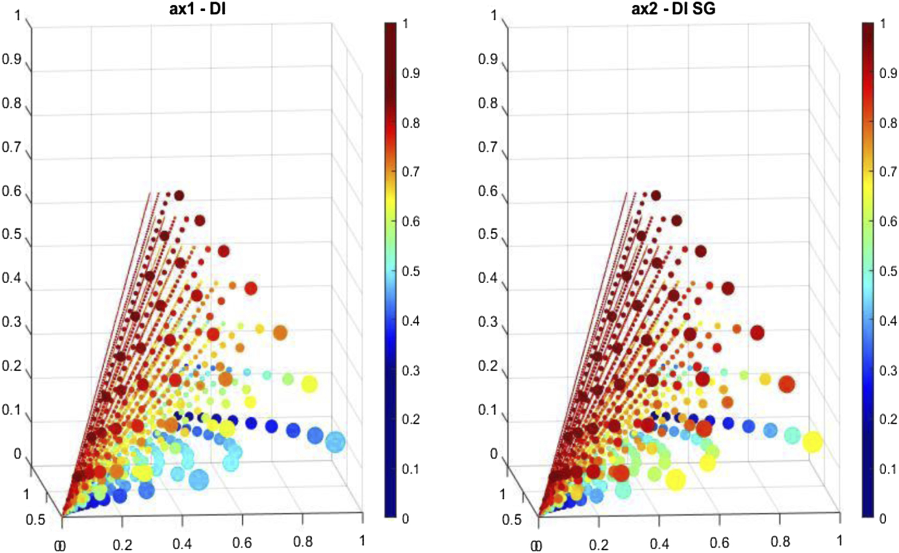
The images show a range of values of m between 3 and 8, and organism numbers ranging between m + 1 and 15. The coloured dots representing values in lines for larger numbers of possible distributions are reduced in size in order to avoid overlap and for ease of viewing. Such an image is best navigated using a 3D interactive format, as is available in Matlab, for example

Even in a 2D representation as an image a clear comparison between values calculated according to the two indices can be made, as well as the variation of the value within a single index as the organisms are distributed among them. For ease of viewing, the size of the coloured dot representing each value has been scaled, so that unit lines containing more distributions are represented by smaller dots. The values of k_φ and k_θ selected for use in figure 1 are $\left.1 /\right.6$ and $\left.1 /\right.8$ respectively.

The figure primarily serves to illustrate the fact that the GSDI generally provides larger values for the diversity index than the PDI, particularly so at lower values for the number of species and organisms. An advantage of the PDI is that it gives lower values than the GSDI in distributions close to or equal to uniform representation in small communities.

It follows from the definition above that the limiting value for the new DI in the case of equally represented species is simply $\frac{m-1}{m}$, contrasting with a value of $\frac{N(m-1)}{m(N-1)}$ for the GSDI. In the latter case, when all species have a single organism representing them the value of the GSDI is 1, which clearly does not present a realistic picture of diversity, being both independent of the number of species present and suggesting 'total' diversity. The value of the new DI in this case depends on the number of species (as required by the conditions provided for its construction) but is independent of the number of organisms present; it may be argued that this gives a more realistic value that represents the distribution of the organisms between the species irrespective of how many (equal) representatives there are for each species. For example, it might reasonably be considered that three species represented by ten organisms each in fact represents no greater diversity than three species represented by a single member each, and this is the sense of diversity captured in the new DI. In this sense, it is closer to a measure of 'species richness'.

Jost [12] introduces the term 'true diversity'—referred to with different names by different authors, for instance the 'effective number of species' by Macarthur [5] and the 'numbers equivalent' by Patil and Tailee [17] in economics. Thus for a given value of the index calculated for a particular distribution, this corresponds to the number of species present if all organisms are equally represented. In this case, the 'true diversity' can easily be shown to be (see appendix B)

$$\begin{equation}\frac{1}{1-{\Gamma}}\end{equation} \tag{ 9 }$$

and this corresponds, in the limit of large N and n_i , to the same value for the Gini–Simpson index. It is interesting to note this expression, while true for all values of species number n_i and number of organisms N for the new diversity index, is only true in the 'large community' limit for the GS index, and this might be considered a point in its favour. Indeed, most of the indices introduced to date may be represented by expressions of the form

$$\begin{equation}\sum\limits _{i=1}^{m}{\left(\frac{{n}_{i}}{N}\right)}^{q},\end{equation} \tag{ 10 }$$

where q is an exponent that varies from one index to another. In consequence, different indices that reduce to an expression of this kind with the same value of q are equivalent, and measures of the true diversity would be the same for such indices, and given by [12]

$$\begin{equation}{}^{q}D={\left(\sum\limits _{i=1}^{m}{\left(\frac{{n}_{i}}{N}\right)}^{q}\right)}^{\frac{1}{1-q}}.\end{equation} \tag{ 11 }$$

These are a generalization of Hill's numbers [18], and the exponent q may be termed the order of the diversity. Thus different functional forms for a diversity index may be connected in this way, with the true diversity being dependent only on the order of the diversity index.

The DI proposed here is not represented in this way, and therefore is not immediately equivalent to indices thus far introduced. It therefore also does not fall under the category of a generalised weighted GS index as proposed by Guiasu and Guiasu [15, 19], and hence their analysis of such generalised functions may not apply here.

Jost [12] introduces a desirable 'scaling' test for an index, proposing that the true diversity calculated for sixteen equally represented species is represented by an index which predicts a value of true diversity twice as large as that for 8 equally represented species. In other words, the true diversity should be proportional to the number of species present. In common with indices defined by expression (10) above, the new DI passes this test. A stiffer requirement is Hill's 'doubling property' [18], which states that for any particular distribution, halving the number of representatives of each species while doubling the number of species (the example that Jost [12] provides is to split each species into two equal groups of males and females and then treat each of these as a separate species) should double the measure of true diversity. A proof provided in appendix B shows that the new DI also passes this more stringent test, although it could be argued that strict doubling in this way is not so meaningful, providing nothing more than a measure akin to species richness and failing to properly take into account the relative representation of common and rare species.

A new diversity index has been introduced which is based on an intuitive set of properties. Values for the new index have been calculated and compared with the popular Gini–Simpson index, and it has been shown that the new index compares favourably with it in providing more realistic values, in particular in predicting the 'true diversity' at low counts of organisms and species. In this instance, these low counts—defining a 'small community'—are when the number of species m is 10 or less and the number of organisms N is 20 or less. At high counts of both of these parameters (the 'large community' limit) the two indices tend to coincide for equally represented species.

The index passes the desirable test of predict true diversity that is equivalent to species richness in the case of equally represented species, and passes also a more stringent test when the species are not equally represented. As noted above, it could be argued that this behaviour is similar to a behaviour equivalent to species richness, which may not be so meaningful when rare species are only minimally represented.

We introduce here also a novel way of representing the space of DI values in a convenient form which permits closer comparison between different formulations of DI in a visual format.

Future work will seek to establish a more efficient counting algorithm for representing the possible distributions, a comparison with a broader range of diversity indices, and application to a broader range of practical problems in order to characterise the behaviour of the index more fully, including also potential use in language applications [20]. We will also seek to extend the work to explore the behaviour of indices where the linear term in equation (3) is replaced by a higher order polynomial, as well as to extend the application to include measures of phylogenetic distance. A further aim of this work is to explore the behaviour of indices of this kind when sampling distributions whose frequencies appear to be predicted on a combinational basis, and which appear to follow a universal distribution [21].

All data that support the findings of this study are included within the article (and any supplementary files).

It is probably easiest to describe the algorithm in the first instance by way of an example. Consider the following example illustrating the distribution of eight organisms among four species. As described above, we need only consider here the remaining organisms noting that four organisms must already respectively represent each species, hence p = 4.

The enumerated distributions follow the pattern below. Note that these values correspond to digit values in a modulo-5 counting base. In general, the values are incremented by a decimal value of 4, and the decimal increase between the previous row and the current one is shown only for those values where the increment differs from 4.

0004

0013

0022

0031

0040

0103 8

0112

0121

0130

0202 12

0211

0220

0301 16

0310

0400 20

1003 28

1012

1021

1030

1102 12

1111

1120

1201 16

1210

1300 20

2002 52

2011

2020

2101 16

2110

2200 20

3001 76

3010

3100 20

4000 120

Recall that these numbers are written in modulo-(p + 1)—in this case modulo-5—and therefore the digits, counting from the least significant to the most significant, represent respectively units, p + 1, (p + 1)², (p + 1)³ etc. Note that each non-uniform jump of 4 occurs when the units digits is zero, as well as when this is zero along with higher place value digits also being zero. Let j represent the digit number, beginning with j = 1 as the units digit, and label the highest non-zero digit as j = q when the non-uniform increment takes place. It may be observed that the increment in these cases corresponds to (p + 1)^q − Z_q (p + 1)^q−1 + Z_q − 1 where Z_q represents the value in the qth digit prior to incrementing. This forms the basis of the algorithm coded in Matlab, whereby the sequence of zero-occupied digits is checked prior to incrementing, and it enumerates precisely the exact number of acceptable distributions without any redundant counts.

Using the example above, it should be clear that, in general, if one unit increments are used (without the zero-checking procedure noted above), the count will reach a maximum of p(p + 1)^m−1. Using a stars-and-bars method (used as early as 1915 by Ehrenfest and Onnes [22]), it is easy to show that the number of distributions that contain the correct digit sum (p) is given by $\frac{\left(m+p-1\right)!}{p!\left(m-1\right)!}$. In the case given in the text of m = 10 and p = 10 (thus N = 20) then the total count corresponds to 2.357 947 691 × 10¹⁰ and the number of acceptable distributions is 92 378.

We follow here an algorithm based on the generalised one provided by Jost [12] in order to calculate the 'true diversity' for any diversity index based on a sum of powers of n_i , the number of organisms of species i, simplified in this instance due to the specified form of the PDI. By formulating an expression for the diversity index Γ of m equally represented species (hence n_i = n₀ $=N /m\left. \right)$ and then solving for m, the required formula for the true diversity (termed D by Jost and equivalent to m in this case) is obtained.

Thus

$$\begin{equation}{\Gamma}=\frac{m-1}{m}\sum\limits _{i=1}^{m}\frac{{n}_{i}}{N}\enspace {\mathrm{e}}^{\left(\frac{N-m{n}_{i}}{N}\right)}\end{equation} \tag{ B.1 }$$

and using the equal representation condition $\left.{n}_{i}=N /\right.m={n}_{0}$

$$\begin{equation}{\Gamma}=\frac{m-1}{m}\sum\limits _{i=1}^{m}\frac{1}{m}\enspace {\mathrm{e}}^{\left(1-\frac{m}{m}\right)}.\end{equation} \tag{ B.2 }$$

The exponent is zero, and the summation total is 1. Hence

$$\begin{equation}{\Gamma}=\frac{m-1}{m}\end{equation} \tag{ B.3 }$$

which is easily rearranged to give the required formula for D, the true diversity.

$$\begin{equation}m=\frac{1}{1-{\Gamma}}=D.\end{equation} \tag{ B.4 }$$

Beginning from the definition of the DI

$$\begin{equation}{\Gamma}=\frac{m-1}{m}\sum\limits _{i=1}^{m}\frac{{n}_{i}}{N}\enspace {\mathrm{e}}^{\left(\frac{N-m{n}_{i}}{N}\right)}\end{equation} \tag{ C.1 }$$

one may label the sum in the formula as S, hence

$$\begin{equation}{\Gamma}=\frac{(m-1)S}{m}.\end{equation} \tag{ C.2 }$$

The true diversity as defined by Jost is given by

$$\begin{equation}D=\frac{1}{1-{\Gamma}}\end{equation} \tag{ C.3 }$$

which in the case of equally distributed species (i.e. when ${\Gamma}=\frac{m-1}{m}$, and S = 1) easily reduces to a value of m.

If 'Hill doubling' is conducted in the manner described by Jost (splitting each species into two equal groups of males and females and then treating each of these as a separate species) then this may be represented in the following way

$$\begin{equation*}m\to 2m\end{equation*}$$

$$\begin{equation*}{n}_{i}\to \frac{{n}_{i}}{2}\end{equation*}$$

$$\begin{equation*}{n}_{i+m}={n}_{i}\end{equation*}$$

and N is unchanged.

Then

$$\begin{equation*}{{\Gamma}}_{\text{double}}=\frac{2m-1}{2m}\sum\limits _{i=1}^{2m}\frac{{n}_{i}}{2N}\enspace {\mathrm{e}}^{\left(\frac{N-2m{n}_{i} /2}{N}\right)}\end{equation*}$$

$$\begin{equation*}{{\Gamma}}_{\text{double}}=\frac{2m-1}{2m}\sum\limits _{i=1}^{2m}\frac{{n}_{i}}{2N}\enspace {\mathrm{e}}^{\left(\frac{N-m{n}_{i}}{N}\right)}\end{equation*}$$

$$\begin{align}{{\Gamma}}_{\text{double}}& =\frac{2m-1}{2m}\left(\sum\limits _{i=1}^{m}\frac{{n}_{i}}{2N}\enspace {\mathrm{e}}^{\left(\frac{N-m{n}_{i}}{N}\right)}\right.\\ & \quad \left.+\sum\limits _{i=m+1}^{2m}\frac{{n}_{i}}{2N}\enspace {\mathrm{e}}^{\left(\frac{N-m{n}_{i}}{N}\right)}\right)\end{align} \tag{ C.4 }$$

and using the property that

$$\begin{equation*}{n}_{i+m}={n}_{i}\end{equation*}$$

this may be rewritten

$$\begin{align}{{\Gamma}}_{\text{double}}& =\frac{2m-1}{2m}\left(\sum\limits _{i=1}^{m}\frac{{n}_{i}}{2N}\enspace {\mathrm{e}}^{\left(\frac{N-m{n}_{i}}{N}\right)}\right.\\ & \quad \left.+\sum\limits _{i=1}^{m}\frac{{n}_{i}}{2N}\enspace {\mathrm{e}}^{\left(\frac{N-m{n}_{i}}{N}\right)}\right)\end{align} \tag{ C.5 }$$

$$\begin{equation*}{{\Gamma}}_{\text{double}}=\frac{2m-1}{2m}\left(\frac{S}{2}+\frac{S}{2}\right)\end{equation*}$$

hence

$$\begin{equation}{{\Gamma}}_{\text{double}}=\frac{(2m-1)S}{2m}.\end{equation} \tag{ C.6 }$$

Since

$$\begin{equation}{D}_{\text{double}}=\frac{1}{1-{{\Gamma}}_{\text{double}}}\end{equation} \tag{ C.7 }$$

then simple substitution gives

$$\begin{equation}{D}_{\text{double}}=\frac{2m}{2m-\left(2m-1\right)S}.\end{equation} \tag{ C.8 }$$

Since D is defined to be the diversity equivalent to a distribution of equally represented species, then S = 1 and D becomes simply 2m i.e. double the original value and hence the Hill doubling criterion is fulfilled.