

Abstract
How bacteria sense local chemical gradients and decide to move has been a fascinating area of recent study. Chemotaxis of bacterial populations has been traditionally modeled using either individual-based models describing the motion of a single bacterium as a velocity jump process, or macroscopic PDE models that describe the evolution of the bacterial density. In these models, the hydrodynamic interaction between the bacteria is usually ignored. However, hydrodynamic interaction has been shown to induce collective bacterial motion and self-organization resulting in larger mesoscale structures. In this paper, the role of hydrodynamic interactions in bacterial chemotaxis is investigated by extending a hybrid computational model that incorporates hydrodynamic interactions and adding components from a classical velocity jump model. It is shown that by including hydrodynamic interactions, a suspension with a low initial volume fraction can exhibit locally high concentrations in bacterial aggregates. Also, it is shown that hydrodynamic interactions enhance the merging of the small aggregates into larger ones and lead to qualitatively different aggregate behavior than possible with pure chemotaxis models. Namely, differences in the shape, number, and dynamics of these emergent clusters.
Export citation and abstract BibTeX RIS
1. Introduction
The study of collective swimming of bacteria has lead to some remarkable experimental observations including enhanced mixing, increased swimming speeds, and novel effective properties of the suspension. The complex interplay between chemically motivated interactions (e.g. chemotaxis) and hydrodynamic interactions is not completely known. Understanding the roles of chemotactic and hydrodynamic effects is important in fields such as biomedicine where researchers investigate the role of chemotaxis in the virulence of gastrointestinal pathogens [1] and the presence of V. anguillarum in waterborne infections in fish [2]. Additional applications include tissue remodeling through collective migration of cells [3] as well as the dynamics of C. jejuni in the gall bladder and intestinal tract [4]. This work seeks to study these interactions at the microscale in order to elucidate the roles of chemotaxis and hydrodynamics in aggregate formation and the resulting dynamics. We also address how chemical and physical cues interact with each other and alter bacterial movement, which is critical in applications such as microfluidic devices [5], drug delivery devices [6], and living liquid crystals [7, 8]. In addition, by understanding this interplay between physical and chemical cues, one can develop gradient sensing synthetic colloids with controllable behavior [9–11]. Specifically, these applications rely on the ability to direct the coordinated behavior of the bacteria to accomplish a task, efficiently decompose harmful chemicals, or form patterns revealing structure formation at a larger scale.
Chemotaxis is the active movement of organisms, such as bacteria, in response to external signals. Specifically, bacterial chemotaxis is crucial in bacteria-associated infections and bioremediation [12, 13]. Bacteria such as Escherichia coli move by alternating forward-moving 'runs' and reorienting 'tumbles' [14, 15]. In the absence of external signal gradients the overall bacterial movement is an unbiased random walk; however, when exposed to a chemical signal, bacteria bias their movement by extending (shortening) their runs in more (less) favorable directions [16]. This modification of movement is governed by an intracellular chemotaxis signaling transduction pathway that involves a rapid response of the bacterium to the signal termed 'excitation' and a slow 'adaptation' that allows the bacterium to subtract out the background signal and respond to further signal changes [17]. When combined with a self-secreted attractant, bacterial chemotaxis can lead to intricate population patterns, including aggregates [18, 19], continuous or perforated rings [20], traveling bands [21, 22], and spiral streams [23].
The formation of aggregates due to chemotaxis has been extensively studied in the dilute limit. Here the run-and-tumble movement of a single bacterium has been described as a velocity jump process with straight runs and brief reorienting tumbles where the run-length biases towards locations with higher concentrations of attractants or lower concentrations of repellents [24]. Also, recent individual-based models of bacterial movement have been coupled with reaction–diffusion equations of external signals to explain chemotaxis-induced bacterial pattern formation [21, 25] and modeling individual microswimmers as simple objects such as dumbbells or force dipoles (e.g. [26–29]). This is in contrast to approaches relying directly on continuum PDEs (e.g. [22, 30–35]) which forgo explicit microscopic interactions from first principles, some ignore the hydrodynamic or collisional interactions between bacteria to simplify computations and analysis. While this simplification is valid in regions where the bacterial volume fraction is low, hydrodynamic interactions can become important when the bacterial volume fraction becomes high. For example, inside an aggregate or a moving band of bacteria the local concentration is much larger. In recent work, it has been found that in the absence of chemotaxis, bacteria undergo collective motion when the bacterial volume fraction reaches 20% [26, 36].
The main focus of this paper is to bridge the gap in current knowledge by investigating the role of hydrodynamic interaction in bacterial chemotaxis and pattern formation. The current literature has examined these effects, but has yet to clearly outline the observed phenomena which are due to purely chemotactic forces and those which require the presence of fluid-mediated hydrodynamic interactions. Recent papers by Lushi et al have introduced a PDE kinetic model that has shown through simulation how hydrodynamic interactions can modify run-and-tumble dynamics associated with chemotaxis [37] and novel pattern formation in [32]. Namely, the onset of instabilities in the uniform state create fragmented regions of aggregation. Futhermore, a recent linear stability analysis suggests that chemotaxis can stabilize hydrodynamic instabilities in active suspension [38]. Further experimental studies have shown that the chemotaxis signaling pathway can drastically change the tumbling bias in a swarming, collective state as opposed to an insolated bacterium [39]. These works cite the need for further systematic studies investigating the interplay between chemotaxis and fluid flow due to self-propulsion that incorporate microscopic near-field interactions, through excluded-volume or collision dynamics, which was not considered in the current continuum framework, but will be incorporated into the present model.
We address this need here by using a first principles mathematical model that combines bacterial movement, fluid motion, and extracellular signal dynamics presented in section 2. This will allow for a direct investigation of the microscale interactions that lead to the different microswimmer dynamics. When the hydrodynamic equations are dropped and the fluid velocity is set to 0, the model reduces to the classical velocity jump model used in [25]. In sections 4.2 and 4.3, we numerically compare the new hybrid model with hydrodynamic interactions (called the 'HI model') and the classical velocity jump model (called the 'VJP' model) given different average bacterial densities in the context of self-induced aggregation. Specifically, we compare the dynamics of aggregate formation, merging, and collective properties. We address the question of under what conditions hydrodynamic interactions, which are computationally more expensive, are needed in modeling bacterial chemotaxis. Stark differences are observed in the behavior of the aggregates with and without the presence of hydrodynamic interactions. Finally, we perform a sensitivity analysis on the model and summarize our results with a discussion of future directions.
2. Mathematical approach
In this section, we extend a recent mathematical model for bacteria that incorporates bacterial movement, fluid flow, and signaling dynamics from [26, 40, 41] by adding an additional component accounting for chemotaxis. The base model was chosen due to its ability to explain experimental observations on the nonlinear viscosity of bacterial solutions, the critical threshold for the onset of bacterial collective motion and distinguish the behavior of motile and immotile bacteria. The modified model used herein will be built by incorporating a classic velocity jump process and the resulting effects on bacterial motion and chemical signal advection by the surrounding fluid. Here bacteria are described as point force dipoles that have finite size enforced via an excluded-volume potential.
2.1. Classic velocity jump process (VJP) model
We briefly review the classic velocity jump model used in previous works such as [42]. Bacteria chemotax by changing their frequencies of tumbling in response to external signal gradients. Biologically, this can be thought of as searching for local surroundings with more favorable conditions. This is achieved through complicated intracellular signaling events triggered by receptor-ligand binding and unbinding and involves internal signal excitation, adaptation and amplification as well as modification of flagellar rotation. In past works, a tumbling rate dependent on the swimming direction has been implemented to enforce chemotatic movement (e.g. [43]). In this paper, we employ a simplified approach that assumes the tumbling rate  depends on the external signal gradient directly [25, 44, 45]. Specifically, we assume
Here  is the external signal concentration at the bacterium location
  . The sensitivity to the chemical gradient is captured in the dimensionless constant
 ![$\kappa \in [0,1]$](https://content.cld.iop.org/journals/1478-3975/17/1/016003/revision2/pbab57afieqn004.gif) and the noise a bacterium may experience in trying to identify the correct chemical gradient is encoded into the constant
and the noise a bacterium may experience in trying to identify the correct chemical gradient is encoded into the constant  . Both parameters help quantify the dependence of bacterial tumbling on the signal gradient. In particular, the noise captured by
  could represent thermal noise in the signal passing through the fluid or a bacterium's inability to completely identify the signal gradient from local chemical measurements. A recent work studying E. coli shows that these sources of noise occur at the interface of the chemical ligands and chemoreceptors can interact with one another resulting in an affect on the chemotactic motility of the bacterium [46]. This work is the first to use the simple form given in (1) to model the modified tumbling rate and it has not been verified for rod-shaped cells prior to this work; however, it captures the essential response of a bacterium and is compatible with the individual-based modeling framework employed here.
The natural, unbiased tumbling rate is given by  . To build intuition for the change in tumbling rate as a function of the chemical signal gradient, we consider the limiting cases. Observe that in the limit of zero noise
  , (1) reduces to
  where the dot product gives the cosine of the angle between the unit vector in the direction of the chemical gradient
  and the bacterium's current orientation
  . Thus, if the bacterium is swimming in the direction of the chemical gradient the tumbling rate reduces to near zero,
  , but if a bacterium is swimming orthogonal to the chemical gradient, then
  and the average time between tumbles increases to the natural, unbiased rate.
Classic works studying the tumbling of E. coli, experimentally observed that the tumbling rate should be proportional to the chemical gradient [47]. Furthermore, this work makes the stronger statement that once a bacterium is swimming in the direction of the chemical gradient the tumbling rate should be decreasing monotonically. The importance of the swimming direction and the magnitude of the chemical gradient are crucial for the individual-based modeling framework and are captured in (1). This is accounted for by observing that in the limit as  the tumbling rate converges to
  which enforces the boundedness of the response to the chemical gradient even if very large. Also, as
  the tumbling rate returns to a value close to the typical isolated constant rate
  where the tumbling rate is linearly dependent on the chemical gradient with stiffness
  (see [44, 48] for alternative modeling approaches where
  is directly proportional to the gradient). This behavior illustrating the stiffness and boundedness of the chemotactic response directly relates to the same response in the chemotaxis flux in the continuum description (e.g. the flux-limited Keller–Segel model). In contrast with the classic Keller–Segel model, the flux-limited Keller–Segel model has solutions which do not blow up in finite or infinite time [49]. This is also related to a linear instability of the kinetic (continuum) chemotaxis model based on the velocity jump process. In relation to bacterial suspensions, the length of a run is decided by the stiff response to temporal sensing of chemical cues [50].
For the simulations presented throughout this work, we take  tumb s−1,
  M mm−3 for comparison with prior results of a classic velocity jump model [25]. To incorporate tumbling in the dynamic equations, it is assumed that during a tumbling event a bacterium chooses a random direction
  instantaneously after stopping with no directional persistence, according to the constant turning kernel

where  is the unit sphere and
  as in [43]. While the classic VJP model (1) and (2) only allows bacteria to perform straight periods of runs followed by a reorientation through tumbling, the approach here will allow for more complex fluid-mediated movement. In particular, bacteria will propel themselves forward, be advected by the local fluid flow generated by other bacteria, and attempt to follow the local chemical signal gradient which is also advected by the fluid.
2.1.1. Bacterial motion
We summarize the remaining components of the thin film quasi-2D model used here and originally developed in [26, 40, 41]. Denote the position of the center of mass and the orientation direction of the ith bacterium by  and
and  . In addition, it is assumed that a bacterium propels itself in the direction
  with relative swimming speed
  . We let
  be the fluid velocity on the location of the ith bacterium, which is modeled as a Stokesian fluid defined in section 2.1.3. Moreover, we introduce a short-range, volume exclusion force
  acting on bacterium i by all other bacteria. The form of
  is of a truncated Lennard–Jones type (for greater detail refer to [26]). In the present model, volume exclusion only occurs when two bacteria are very close to each other to prevent them from occupying the same region. An alternative approach accounting for similar forces using squirming spherical swimmers has been considered in [51]. For simplicity we assume any excluded-volume interaction acts in the direction of the centers of mass of each bacterium resulting in no effect on bacterial orientation. By neglecting inertia, we arrive at the following system describing bacterial motion during a run
where  is the drag coefficient for the bacterium, representing an effective Stokes' Law relating a force to a velocity at low Reynolds number, and N is the total bacterium number.
The fluid flow can also change the direction of the bacterial movement. We assume that the bacteria are ellipsoids with major and minor axes denoted as a and b. The governing equation for  during a 'run' is given by Jeffrey's equation [52]
Here  and
and 
![$[\nabla_{\bf x} {\bf v}({\bf x}^i)]^T\}/2$](https://content.cld.iop.org/journals/1478-3975/17/1/016003/revision2/pbab57afieqn036.gif) are the vorticity and rate of strain respectively of the flow induced by all other bacteria on the location of the ith bacterium, and
are the vorticity and rate of strain respectively of the flow induced by all other bacteria on the location of the ith bacterium, and  is the Bretherton constant accounting for the bacterial shape (with B = 0 for spheres and B = 1 for needles). The derivation of equation (4) and further details of the physical implications can be found in [26, 29, 52, 53].
Incorporating the directional jumps due to tumbling into (4), we formally obtain
where  are independent random variables uniformly distributed on
  and
and  are independent inhomogeneous Poisson processes with intensity
  . In this work, the only random component of motion comes from the tumbling mechanism. In principle, one could consider random fluctuations, but these effects appear minimal compared with the swimming motion and tumbling.
2.1.2. Signal dynamics
The tumbling frequency of a bacterium is determined by the external signal  . In this paper, we consider the situation in which there is no external signal, but rather the signal is secreted by the bacteria and causes the bacteria to aggregate as demonstrated experimentally in [54]. The chemical signal is then advected by the fluid itself. Thus, the governing equation is a reaction–diffusion–advection equation for
  for
for 
Here  is the diffusion coefficient of the signal, fsec is the secretion rate by a single bacterium, and
  is a constant degradation rate. The advection term
  describes the dispersal of the signal due to the fluid motion and can be simplified to
  due to the incom- pressibility of the fluid. The parameters are taken as
  mm2 s−1 [55],
  M s−1 per bacterium, and
  s−1 similar to the parameters leading to aggregation in the purely chemotaxis model presented in [42, 56].
2.1.3. Fluid flow
Observe that the typical size of a bacterium under consideration (e.g. E. coli) is 1–2  m and each bacterium is capable of swimming at speeds up to
  in isolation [26, 36]. Given these values the Reynold's number of the suspension is Re
 . In addition, the time scale for the flow to reach its steady state is much smaller than the characteristic time scale for bacterial swimming. Based on these considerations, the fluid is governed by a linear Stokes equation which must account for a bacterium confined to a thin layer of fluid. An explicit analytical expression for the fluid velocity generated by a Stokeslet (point force monopole) in a thin film of thickness w satisying Stokes equation has been derived by using the method of images in [57] and simplified to an expression for the flow in the xy-plane (z = 0) in [58]. Following a similar procedure, the dipolar solution can be obtained by taking the flow due to two oppositely oriented force monopoles and letting the distance between them go to zero as in [26]

where  is the distance from the dipole location to the origin in the xy-plane. Here the prefactor
  has units of length4/time while
 ![$\nabla^3[\log(r)] : {\bf d}{\bf d}$](https://content.cld.iop.org/journals/1478-3975/17/1/016003/revision2/pbab57afieqn058.gif) has units of 1/length3. This pre-factor contains the physical quantities of the dipole moment U0, the film thickness w, the ambient fluid viscosity
has units of 1/length3. This pre-factor contains the physical quantities of the dipole moment U0, the film thickness w, the ambient fluid viscosity  . Here
  is a function of the depth and has a parabolic profile h(z) = c(z)w2 where c is quadratic in z [57]. At z = 0,
  , where
  m. Thus, in the computational domain (xy-plane, z = 0)
  . As opposed to a completely two-dimensional formulation which has a fundamental solution
  , the quasi-2d suspension decays as 1/r3 due to the confinement of the suspension. This results in a three-dimensional suspension where the z-dimension is considered to be much smaller than the x and y dimensions,
  , giving it a quasi-two-dimensional appearance (see figure 1). A much more detailed explanation of the model formulation for the fluid velocity can be found in the authors previous works [26, 40, 41].

Figure 1. Depiction of thin film fluid layer with swimming bacteria. Here bacteria are free to move and interact. As bacteria swim they generate flows which can effect the movement of other nearby bacteria and advect any chemical secreted by the bacterium.
Download figure:
Standard image High-resolution imageThis allows for a two-dimensional simulation in which three-dimensional features are encoded into the coefficient through Ku. This approach compares qualitatively well with the streamlines observed in recent experiment (see figure 2 and [59]). Using the linearity of Stokes equation, we approximate the true fluid flow  from N bacteria at location
  by the superposition of thin film solutions (6) for a single dipole
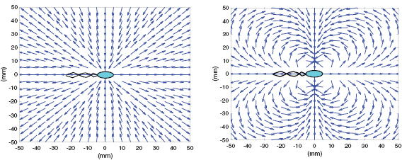
Figure 2. Normalized unit streamlines from the Left: free space (e.g. used in [29]) and Right: quasi-2d thin film solution in (6) matching experimental observations seen in Drescher et al [59].
Download figure:
Standard image High-resolution imageBy considering pairwise interactions between the force dipolar representations of the bacteria in the semi-dilute regime, the flow generated by all the bacteria is simply the superposition of the flow generated by each cell. Semi-dilute models combined with an excluded-volume potential as implemented in this work have been successfully used to study many concentration regimes (e.g. see [26, 41]). In those recent works among others, the model starts to break down at extremely high concentration (>70% area fraction) due to the dominance of near-field forces over hydrodynamic. We save the discussion of the high concentration regime and the resulting effect on the distribution of the chemical for appendix C, since it diverts from the focus of this work on the semidilute regime.
2.1.4. Advantages of modeling approach
The modeling approach used here offers many advantages over past studies of chemotactic aggregation using continuum PDE models such as [32, 37, 43]. Foremost, the microscopic approach used here is developed from first principles where the dynamic equations (3) and (4) are derived from a balance of forces and torques on the particle. This allows for explicit hydrodynamic interactions between bacteria and enables the use of an excluded-volume potential to incorporate some features of near-field interactions absent from the past approaches. Also, this individual-based model is capable of performing side-by-side comparison with real experimental data. In fact, recent studies on collective motion show quantitiative and qualitatively favorable comparison of this modeling approach with recent experiment works [26, 29, 40, 41]. In addition, modeling a bacterium as a point dipole allows one to only track the center of mass and orientation of each cell, greatly reducing the computational complexity. This approach combined with explicit time-stepping numerical methods allow for parallelization of the simulations. This, in turn, allows for simulations consisting of many swimming individuals ( –105) representing a computational domain closer to that of experimental observations. Finally, the microscopic approach is highly flexible in that one can probe the effect of individual parameters or interactions on the macroscopic behavior (e.g. see supplemental material appendix B (stacks.iop.org/PhysBio/17/016003/mmedia)) and allow for the study of general fluid flows unlike [43]. A previous work also cited the benefits of individual-based modeling approach in incorporating stochasticity or fluctuations in the bacterial density field; though, that work focused on the formation of rings through chemotaxis and unlike the present model did not consider the effects of hydrodynamic interactions [56].
3. Numerical approach
In sections 4.2 and 4.3, we present numerical results for comparing the hydrodynamic model (1)–(6) to the purely chemotactic velocity jump process model (1) and (2). The general behavior of the reduced two-dimensional model is qualitatively similar to the full three-dimensional simulations and, indeed, many occurances of collective behavior observed in experiment are quasi-two-dimensional [36, 54, 60]. In practice, we will not be able to solve the problem in an infinite domain, and instead consider a square computational domain [0,L]2 with periodic boundary conditions imposed on the fluid velocity  and signal S. For the bacteria, this means that if a bacterium exits the domain from one side, it will enter from the corresponding periodic location on the opposite side. In an actual experiment, the fluid may have a hard or semi-solid boundary to hold it in place giving no slip conditions, but the current approach allows one to minimize any boundary effects and simulate the behavior in the bulk of the suspension far from the suspension boundaries. In general, models of this form are well-posed due to the presence of the excluded-volume constraint [53]. In the absence of such a constraint, the hydrodynamic forces could cause two neighboring cells to attract each other resulting in a singularity in the interaction force.
The fluid velocity in a domain with periodic boundary conditions can be represented using the method of images, by summing over all periodic translations of each bacterium
where  is defined in (7). Numerically, we approximate
  by truncating the infinite series at large
  , e.g.
where  mm. The R was chosen due to numerical observation: Beyond this distance the resulting change in the fluid velocity was less than
  of the magnitude. The parameter values used in our simulations are summarized in table 1 and are drawn from recent studies (e.g. [26, 36, 42, 52]).
Table 1. Biological quantities used in model and simulation.
| Symbol | Dimensional value | Description | Reference |
|---|---|---|---|
| T | 2 hrs (7200 s) | Real-time sim. length (s) | |
| L | 1.5 mm | Side length of domain | [36, 42] |
| a | 1  m m |
Radius of bacterium body | [36] |
 |
20  m s−1 m s−1 |
Isolated cell swim speed | [36] |
 |
10  M M |
Crossover concentration (absolute/relative) sensing | [56, 61] |
| B | 0 | Bretherton constant (Spheres) | [52] |
| w | 10  m m |
Film thickness | [36] |
 |
1 s−1 | Tumbling rate | [42] |
 |
.9 | Response rate to chemical gradient | |
 |
 M mm−3 M mm−3 |
Sensitivity to chemical gradient | |
 |
 mm2 s−1 mm2 s−1 |
Chemical diffusion strength | [42, 55] |
| fsec |  M s−1 M s−1 |
Chemical secretion rate | [42] |
 |
 s−1 s−1 |
Chemical degradation rate | [42] |
 |
Ratio repulsion potential depth / drag coefficient | [26] | |
 |
1  m m |
Volume exclusion radius | Exp. Est. |
 |
 sec sec  m−2 m−2 |
Drag Coefficient | Exp. Est. |
| Ku | .531  m4 s−1 m4 s−1 |
Velocity pre-factor | Exp. Est. |
In the simulation results, we assume that bacteria are spherical unless otherwise stated. This assumption will remove any effect shape has on the qualitative behavior of clusters allowing one to focus on hydrodynamic interactions and chemotaxis. A brief discussion of how shape may effect the results presented can be found in supplemental material appendix B. The numerical algorithm combines simulation of continuous bacterium trajectories with the discretization of the PDE signal equation (5) on a finite difference mesh. The method is an extension of the numerical method used in the case of the velocity jump model in [42]. The combination of the mesh-free motion of the bacteria with the PDEs governing signal dynamics (solved on a mesh) classify this as a hybrid numerical method.
The simulations use  as the characteristic length scale and t0 = .1 s as its characteristic time (roughly the time it takes for a bacterium to swim its body length). This gives a characteristic velocity
  m s−1. The computational domain is taken to be
  or
or  . Even though the HI model for an individual bacterium and each interaction is simple, the suspension consists of 104–105 bacteria resulting in
  pairwise interactions. Observe that the dimensional value of
  m4 s−1 used in the simulations combined with the viscosity of water
  pN · sec
  m−2 and bacterium length
  m we can estimate the dipole moment
This corresponds to a propulsion force  pN which is comparable to the propuslion force captured experimentally from the observed flow from an isolated E. coli bacterium (.42 pN reported in [59]).
The numerical procedure consists of three main parts: (i) evolving particle positions/orientations, (ii) handling chemical secretion and advection in the fluid, (iii) Implement the biased tumbling procedure using the chemical gradient.
- (1)Initially N bacteria are placed within the computation domain [0,L]2 at random (non-overlapping) positions
 with random orientations .
 - (2)
- (3)
- (4)
- (5)Bacteria are checked to see if they tumble according to their modified tumbling rate (1).
- (6)Repeat steps (2)–(5) to march forward in time.


Remark 1. Additional simulations were run where bacteria secreted chemical before updating their position and there proved to be no quantitative or qualitative difference in the observed results as long as the time and spatial scales used were on the order of the baseline values used in this work.
3.1. Chemical secretion and ADI method
To handle the chemical secretion by the bacteria one would need to solve the coupled ODE/PDE system for bacterial movement and signal dynamics. To simplify the numerical approach we implement a so-called semi-discrete algorithm where we continuously solve the ODE equations of motion (3) and (4), but use a finite difference approximation to solve the chemical PDE (5). The bacteria are free to move continuously about the computational domain, but the finite difference scheme relies on the chemical concentration at discrete grid points. In order for the scheme to work well we need to account for two things: (i) the distribution of secreted chemical to neighboring grid points and (ii) an accurate representation of the chemical gradient,  needed for the biased tumbling rate
  in (1).
To answer the first point, we consider the relative amount of chemical near each grid point. Since the bacteria can move freely throughout the computational domain, we assume the signal secreted at a given time appears at the bacterium's present location. In order to capture the true chemical concentration we cannot apply a constant concentration at each of the four nearest grid points, because the gradient used in the tumbling dynamic would be far from reality. Instead, we use the location of the bacterium to compute the appropriate weights on each of the four nearest grid points so that the total amount secreted is consistent with biological considerations. Therefore, the grid points nearest the bacterium receive most of the signal, which is closer to reality, see figure 3.
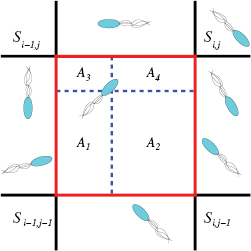
Figure 3. Illustration of the computational domain. The bacteria are free to move continuously in space and are tracked via their orientation  and their center of mass
  . However, the chemical concentration is a discrete quantity defined on the grid. When a bacterium secretes signal the relative weights displayed in the diagram determine the amount at each grid point.
Download figure:
Standard image High-resolution imageNumerically the equation for the signal (5) is solved using an ADI (alternating direction implicit) method, which is a multi-dimensional version of the Crank–Nicholson method. It is easier to solve the problem numerically using the non-dimensional equation (A.3) with full derivation in appendix A. The position of a bacterium inside the computational domain is given by  . At each time step a bacterium secretes a given amount of chemical signal
  . This must be interpolated into a local chemical concentration S, deposited at the neighboring discrete grid points (see figure 3). For a bacterium inside a square subdomain with top right vertex
  the total amount of chemical a given bacterium senses at its location is based on weights given to the four grid points
Here  is the interpolated chemical concentration, A = dx2 is the total area occupied by the bacterium, and the sub-area of each bacterium is Ak for
  . The quantity Ak/A is the fraction of the square occupied by subdomain Ak. The complete step-by-step procedure can be found in [42], but here we provide the idea. The additional chemical secreted by a bacterium is added to the four neighboring grid points based on its location at each time step is
  at
at  ,
,  at
at  ,
,  at
at  ,
,  at
at  , and 0 otherwise Here
  is the amount of chemical secreted by a bacterium and
  is the concentration of chemical secreted into the square subdomain containing the bacterium. This method has also been shown to be unconditionally stable for multi-dimensonal diffusion and heat condution problems as well as being second order in time and space (e.g. [62, 63]). It has also been shown to produce results consistent with experimental observation of E. coli aggregation as noted in [25, 64].
To address the second point we need an accurate numerical representation for the gradient of the signal,  . The biased tumbling rate depends crucially on the chemical gradient. Thus, we must extend beyond the methods outlined in [42] to consider a weighted gradient using the discrete grid points
  . This is done by incorporating more neighboring bacteria and approximating the partial derivatives present in the gradient by central differences.
This has been successfully implemented in a similar case with regard to bacterial chemotaxis in [42]. Just as in the case of bacterium secretion, we want to give more weight in the central difference approximation to the derivative nearest to the bacterium, but all should contribute to the total discrete gradient of S. Thus, this spatial grid choice is important, if too fine then the local gradients are only determined by the chemical contributions of individual bacteria, but if too coarse then bacteria do not have enough time to leave their local subdomain before secreting again. The spatial grid used for the finite differences in the chemical equation in the simulations is  . Observe that the amount of chemical secreted needs to be scaled with the spatial grid to ensure the desired concentration among the local grid points.
4. Results and discussion
We aim to determine the role of hydrodynamic interactions in the self-organization behavior in bacterial populations such as aggregate formation, merging, and the collective movements of aggregates. To do that, one can compare the population dynamics with and without the hydrodynamic interactions using the full HI model presented in section2 (1)–(6) and the classic velocity jump model (VJP) (1) and (2). The VJP model can be obtained from the HI model by removing the hydrodynamic interactions (i.e. setting the fluid velocity  ) and the volume exclusion. Common to both models is self-propulsion, signal secretion, and biased random tumbling.
In terms of computational efficiency, the VJP model is far superior because it does not rely on calculation of the local fluid velocity induced by bacterium movement. The motion of each bacterium in the VJP model is completely independent of all other bacteria at a given time step. To compute the local flow in the hydrodynamic model, one must calculate the flow generated by each pair of particles, resulting in  computations each time step. While the VJP model is highly efficient, it lacks the ability to account for advection of the chemical signal by the fluid. Using numerical comparisons, one can determine under what conditions the computational complexity associated with the more detailed HI model is worth the additional computational time.
4.1. Single bacterium dynamics
One of the advantages of the individual-based modeling approach used throughout this work when compared to continuum modeling with PDEs is the ability to investigate individual bacterium trajectories in time. Before considering the macroscopic dynamics and pattern formation for the bacterial suspension, we investigate the effect of including hydrodynamics on individual bacterium motion. It is observed that for early times when the cells only begin to secrete chemical into the environment the trajectories in each model are basically the same. Since the chemical concentration is small the advection term in (5) has only a small contribution and the magnitude of S remains small in (1). Thus, the tumbling rates in each approach remain the same producing similar trajectories given the same initial data (see figures 4(a) and (b)). The effect of hydrodynamics is not prevalent until the post-aggregation phase when large groups of bacteria secrete chemical signal in one location. The advection term has the ability to distribute the signal to larger areas of the surrounding medium leading to larger area coverage by a bacterium governed by hydrodynamic forces (see figures 4(c), (d) and appendix C). At later times, in a chemical rich environment, we observe that individual dynamics can differ in terms of area covered. Also, the effective tumbling rate is reduced on average by  when hydrodynamic effects are incorporated (1 s−1 in the VJP model to .82 s−1 in the hydrodynamic model on average).
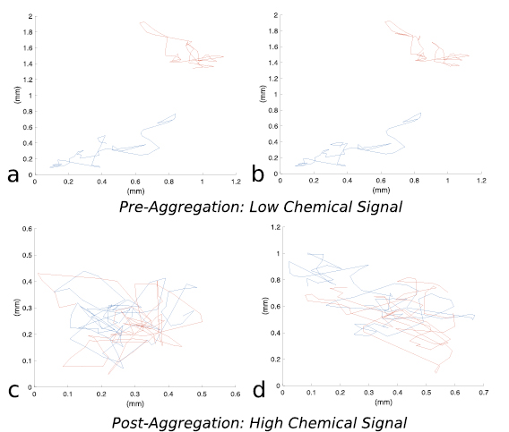
Figure 4. Single bacterium dynamics for two individuals over 100 s of time. Pre-aggregation phase: (a) Bacterium motion at early times (0–100 s) in pure chemotaxis VJP model, (b) bacterium motion at early times (0–100 s) in hydrodynamic model. Post-aggregation phase (c) Bacterium motion at late times (7100–7200 s) in pure chemotaxis VJP model, (d) bacterium motion at late times (7100–7200 s) in hydrodynamic model.
Download figure:
Standard image High-resolution image4.2. Aggregate formation and merging
We begin by showing that starting from a uniform bacterial distribution with no external signal in the domain initially, bacteria can self-organize into aggregates in response to the self-secreted signal, and small aggregates can merge into large aggregates gradually. This is done by comparing the two models outlined above. Throughout this section, we compare a typical realization of each model as well as the average behavior. When a single realization is depicted, the same two simulations are used in all the figures.
Both models were simulated on a 1.5 mm by 1.5 mm domain with periodic boundary conditions, assuming no initial chemical signal,  . The simulations contain N = 7400 circular bacteria randomly placed in the computational domain, corresponding to an average volume fraction
  (see figures 6(a),(d)). Both models predict that bacteria form aggregates within minutes with size comparable to observations in experiments (5–10 bacteria lengths) [42]. Figure 5 shows the early population dynamics typically found in each model. Aggregates start to form around t = 7 min with diameter
  –
– (figures 6(b) and (e)). By t = 13 min, almost all aggregates are well-defined (figures 6(c) and (f)). This is consistent with the observation of complex fluid flows and fragmented aggregation regions observed for 'pushers' (propulsion actuated from behind) using a continuum approach in [37].
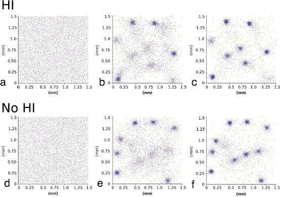
Figure 5. One realization of simulations for t = 0 min (a),(d), t = 7 min (b),(e), t = 13 min (c),(f). (a)–(c) Hydrodynamic model with excluded volume, (d)–(f) Velocity jump model. Initial uniform distribution with volume fraction  . The hydrodynamic effects do not show a large difference in bacterial chemotactic dynamics at short times, but do so at larger time scales as seen in sections 4.2 and 4.3.
Download figure:
Standard image High-resolution image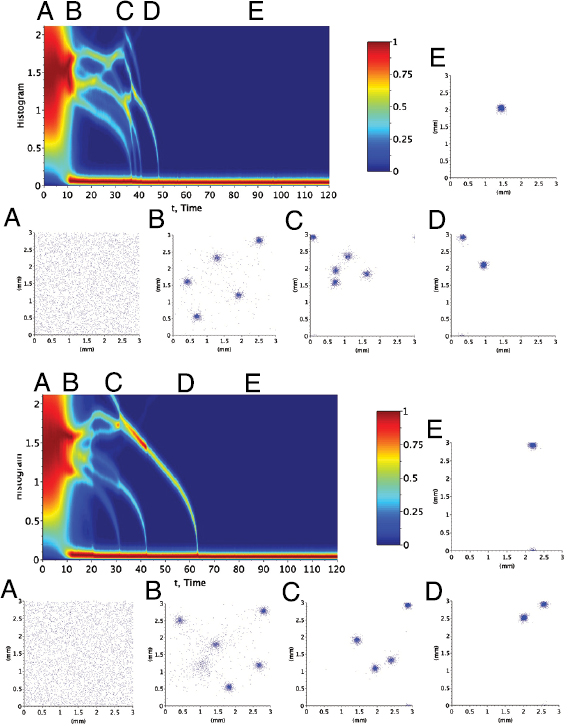
Figure 6. 'Heat Map': histogram of pairwise distances versus time t for the (a) hydrodynamic (HI) model and (b) velocity jump (VJP) model. Observe that it takes longer for aggregates to merge when relying only on chemical signaling.
Download figure:
Standard image High-resolution imageEach aggregate produces a large amount of signal which then attracts isolated bacteria and other aggregates towards it. As time progresses, all the aggregates begin to move as a collective unit and start to merge. Interestingly, the HI model predicts a faster merging process than the VJP model. To illustrate this, we calculated the distribution of the pairwise bacterium distances dij as a function of time. Figure 6 plots the heat maps of these distributions and displays the corresponding bacterial configuration at five moments in time for each model (HI versus VJP). The horizontal red stripes near the t-axes represent the characteristic distance within a single aggregate. The other horizontal stripes represent characteristic distances between aggregates. The vertical lighter branches that collapse into the horizontal red strips represent the merging of two or more aggregates. From figure 6(a), we see that in the HI model realization (figure 6(b)), the initial aggregates start to merge around t = 7 min and by t = 48 min the whole population collapses into a single aggregate. However, in the VJP model realization, the initial aggregates begin to merge around t = 7 min, but the whole population only merges into a single aggregate around t = 65 min.
In order to explain the enhanced merging speed in the hydrodynamic model we must understand what the flows around each bacterium look like. When two bacteria are close to each other and aligned side-by-side, they weakly attract each other due to hydrodynamic interactions, as suggested by the fluid streamlines in figure 2. It has been shown that when the bacterium volume fraction exceeds a threshold (∼20% for bacteria), this weak attraction leads to the onset of collective bacterial motion [26, 36].
Using a simple algorithm to count the number of aggregates by identifying groups of bacteria within one cell length of each other, we can then define a merge event when the cells of one cluster are within two bacteria lengths of another cluster for a significant period of time (on the order of minutes). The results show that with hydrodynamic interactions and the advection of the chemical by the fluid incorporated, the time between the merging of any two aggregates tmerge and the time to form a single aggregate tagg are significantly less than in the pure chemotaxis model. For the hydrodynamic model  and the average time between any single merge event is
  . For the pure chemotaxis model
  and the average time between a single merge event is
  . The discrepancy in merge times is due to the chemical signal advection in the fluid. This allows each bacterium to find a strong chemical gradient faster leading to an increased rate of aggregate formation and merging. Whereas in the pure chemotaxis case, clusters appear to merge only if they happen to be close to each other as they move in time. This is further explained by considering recent results on enhanced mixing and fluid instabilities due to the hydrodynamics flows generated by motile cells in suspensions observed in Saintillan et al [34, 65]. These striking physical features would not be present in the pure chemotaxis model where the dynamics of the fluid cells and associated instabilities are ignored.
Next, consider the evolution of the number of aggregates in time displayed in figure 7(a) for each model. If bacteria are within two bacterium lengths then they are said to belong to the same group. To identify all groups, we start with the first bacterium, label it group one, then label all bacteria within two bacterium lengths of that bacterium group one. We then repeat this process until there is no other bacteria that qualify to be in group one. Then we move to the next bacterium that is not associated with group one, label it group two, and repeat the above process to find all groups. Groups consisting of more than  of the bacteria population are referred to as aggregates or clusters. In figure 7(a), the lines represent the average over ten realizations of each model and the error bars indicate the standard deviation. We note that the two curves agree very well for the first 10 min, but as time progresses the HI model predicts faster merging of these aggregates. In the longtime limit in both cases there should be one large aggregate, but the intermediate behavior is different.

Figure 7. Comparison of the two models with volume fraction  . (a) The number of aggregates versus time. The HI model (red curve) predicts faster merging of aggregates than the VJP model (black curve). (b) Both models predict that the peak volume fraction exceeds the threshold for collective motion before t = 20 min, but after this time the behavior begins to deviate.
Download figure:
Standard image High-resolution imageTo demonstrate whether collective motion occurs during aggregate merging, we compute the peak volume fraction over the entire computational domain as a function of time for each model. To calculate the peak volume (indeed, in 2D the area) fraction, we divide the whole domain into boxes of dimension  m
m  60
60  m and calculate the average volume fraction inside each box. We then take the maximum volume fraction over all the boxes and call it the peak volume fraction at that time. Figure 7(b) shows the statistics for both models suggesting that the peak volume fraction predicted by the two models agrees well for t smaller than 10 min, but the HI model predicts a larger peak volume fraction for larger time, due to the faster merging of aggregates. Intriguingly, the peak volume fraction predicted by both models eventually exceeds the collective motion threshold and the behavior of the two models start to differentiate after the threshold is achieved. This is due to the fact that the hydrodynamic interactions and the fluid advection enhance the alignment and collective swimming of nearby bacteria and this effect is not present in the pure chemotaxis model. In addition, in each case, the peak volume fraction approaches a constant value in time indicating the single aggregate roughly maintains a constant volume fraction. This is consistent with the previous work in [32, 37] where the flow instability generated from hydrodynamic interactions suppressed growth in concentration.
To further understand the role of collective motion in aggregate merging, we simulate a case with much fewer bacteria in the domain. The results with an average volume fraction ten times smaller than the simulations in figure 7 are plotted in figure 8. We see that the statistics of aggregate number and peak volume fraction predicted by the two models match well in general and for each model the threshold for collective motion was never reached. This suggests that as long as the bacterial volume fraction is below the threshold for collective motion the hydrodynamic model and the VJP model demonstrate similar behavior in aggregate formation and merging. Further, the computational complexity involved with the hydrodynamic model is not needed.
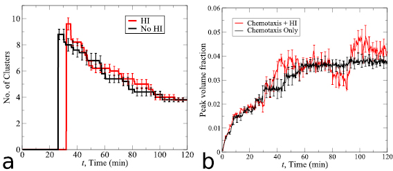
Figure 8. Comparison of the two models with volume fraction  . For low volume fractions the behavior between the models is the same. Each model leads to local concentrations below the threshold for collective motion.
Download figure:
Standard image High-resolution image4.3. Dynamics of a single aggregate
We next investigated the population behavior after all the bacteria merge into a single aggregate using both the HI model and the VJP model. In particular, figures 9(a)–(c) shows the shape of the final aggregates predicted by the two models. The HI model leads to an amorphous aggregate that can change shape over time due to the advection of the chemical by the surrounding fluid and the tendency of the bacteria to swim toward high concentrations of chemical collectively when the local density is large. The VJP model predicts a radially symmetric aggregate in which bacterium motion is solely governed by the local chemical gradient. The agent-based model used throughout this work explains the discrepancy through the hydrodynamic interactions. Unlike in the VJP model, when hydrodynamic interactions are present we observe that local groups of swimmers may move together in a direction other than the cluster center due to the advection of the chemical by the fluid before being attracted back by the chemical gradient. This is clearly observed in figure 9(b) and is only possible with the individual-based modeling approach. This gives insight into the amorphous shape; namely, the chemical concentration distribution is also non-symmetric and moving away from the aggregate center in some directions. Thus, portions of the aggregate move toward these higher concentrations creating the non-symmetric shapes and 'appendages' that grow out from the aggregate center in time. This is not possible in the VJP model because the chemical is not advected by the fluid and simply remains primarily at the center of the cluster forming the outward symmetric shape.
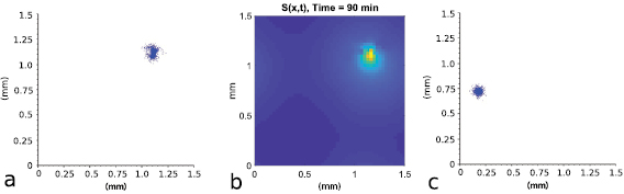
Figure 9. Shape of the aggregates. (a) The hydrodynamic model predicts an amorphous aggregate that changes shape over time. (b) The local chemical concentration at the same time illustrates the origin of this non-symmetric shape. (c) The VJP model predicts essentially a radially symmetric aggregate.  .
.
Download figure:
Standard image High-resolution imageThis effect can only partially be explained by observations from the continuum model in [37] which shows that aggregates leading to high volume fractions create a destabilizing active stress resulting in unsteady flow. This is consistent with figure 9 which shows the high density cluster partially splitting into arms and recombining due to chemotaxis (see also the supplemental movies). For an explanation of why this occurs we return to single bacterium dynamics as discussed in section 4.1 where the advection term in (5) in a chemical signal rich environment leads to drifting trajectories of single cells away from the aggregate. This may also contribute to the amorphous shape and arms extending out from the aggregate body in the hydrodynamic case. The size of the aggregates predicted by both models are about the same, indicating that the intrinsic aggregate size is dictated by chemotaxis or the physical size of the bacterium.
Once all the bacteria form a final aggregate, they can move as a single entity. This has also been observed in recent experiments by Saragosti et al where chemotactic bacteria form traveling bands or rings swimming collectively toward high signal concentrations [66, 67]. To track this collective movement, we recorded the center of mass and investigated whether the aggregate exhibits any type of diffusive behavior. Specifically, we computed the diffusion coefficient D and exponent  from mean-squared displacements
  in figure 10. For the HI model, the diffusion exponent is 1.2–1.3 and the diffusion coefficient of
  . These values indicate super-diffusive behavior as suggested by experiments [68, 69]. In contrast, the VJP model seems to predict a much smaller diffusion exponent
  and coefficient
  . This confirms that the VJP model is not capable of exhibiting collective swimming even in dense aggregates and the aggregates themselves do not display any super-diffusive behavior. Figure 11 plots the aggregate trajectory during one hour of time for one particular realization for each model. Clearly we see that the HI model predicts a more profound movement of the aggregate over time and the VJP model predicts a stationary aggregate located at the highest concentration of chemical secreted.
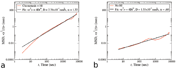
Figure 10. Mean squared displacement of aggregate center of mass ![$\langle [r(\tau+t) - r(t)]^2 \rangle$](https://content.cld.iop.org/journals/1478-3975/17/1/016003/revision2/pbab57afieqn157.gif) versus Time t for (a) hydrodynamic model and (b): velocity jump model. Here
versus Time t for (a) hydrodynamic model and (b): velocity jump model. Here  . Hydrodynamic model displays super-diffusive behavior while the VJP model displays sub-diffusive behavior.
Download figure:
Standard image High-resolution image
Figure 11. Trajectory of the aggregate center in 1h time window in one realization. (a): HI model. (b): VJP model.  .
.
Download figure:
Standard image High-resolution image4.4. Numerical convergence
The baseline time step is .1sec and the spatial step is  m (on the order of a bacterium length). Additional realizations under the same initial conditions were run with spatial and time steps twice as large and half as large. The results show no large qualitative or quantitative difference in average peak volume fraction (range from .521–.571), transition time to cluster formation (5.2–10.1 min), and peak cluster number (8–10 initial clusters). For a thorough sensitivity analysis of the effect of the model parameters on the results please see appendix B.
5. Conclusions
In this paper, we investigated the role of hydrodynamic interactions between bacteria in self-organization patterns due to chemotaxis. This was achieved by comparing the classical velocity jump model (VJP) to a recent hydrodynamic model (HI) developed by the authors with an additional chemotaxis component added. In the VJP model, a bacterium performs a run-and-tumble motion with a bias toward the direction of the concentration gradient. The VJP model was by far the most computationally efficient model and shows aggregate formation on time scales comparable to experiments. The HI model extends the VJP model to include hydrodynamic and excluded-volume interactions between bacteria. It also includes the fluid advection of the chemical signal secreted by the bacteria. Simulations with the HI model are more time-consuming due to the necessity to compute the fluid flow. We sought to understand when these features would lead to novel macroscopic behavior and justify the added computational complexity of the HI model.
We compared the two models based on three main criteria: aggregate formation due to a self-secreted signal, merging, and final aggregate movement. Our results suggest that the two models agree well when the bacterium volume fraction is small so that hydrodynamic interactions become secondary to the chemical gradient attraction. However, once the threshold for collective motion is reached the two models demonstrate different population level (macroscopic) behavior. This suggests that for low volume fractions (e.g.  ) the added complexity of incorporating the fluid equations and hydrodynamic interactions is not necessary to capture the population dynamics and the VJP model suffices, but once the threshold for collective motion is reached, a modeling approach incorporating hydrodynamic interactions is needed.
The individual dynamics of cluster formation in experiment have not been specifically probed and this work lays the foundation for experimentally testable predictions. The HI model predicts a faster merging of aggregates than the VJP model and the onset of which occurs much earlier. In addition, super-diffusive motion of the aggregates is primarily due to collective swimming of the bacteria consistent with experimental observation in [66] and non-isotropic shape of the aggregates due to flow instabilities as in [32, 37]. Here collective swimming occurs after the aggregates are formed raising the local volume fraction beyond that which is needed to observe self-organized swimming behavior (e.g. greater than  volume fraction). We have also provided additional justification through first principles microscopic modeling with excluded-volume constraints that the hydrodynamic flows generated by swimming bacteria modify chemotactic aggregation, limit aggregate concentration, and decrease aggregate merge times as first predicted in [37].
5.1. Biophysical insight
The microscopic modeling approach here has provided new biological insight into the aggregation formation process and resulting dynamics. First, recent experiments have determined that chemotactic bacteria can swim collectively along a concentration gradient [66]. The work here shows that in the absence of hydrodynamic interactions the aggregates become stationary and radially symmetric. Also, we observe that hydrodynamic flows lead to instability in the aggregate shape allowing a segment of the aggregate to extend and move the cell in a given direction. Observations of the specific configuration of dense aggregates are not possible with a continuum modeling approach. The microscopic model here also provides more insight into why the peak volume fraction becomes constant in the single aggregate setting. While models with and without hydrodynamic interactions can lead to temporary spikes in bacterial concentration at locations of high chemical signal, the excluded-volume constraints cap the maximum volume fraction at the packing fraction for circles in two dimensions (bacterial peak volume fraction approaches  –.8 and the maximum packing fraction for spheres is
  ). The excluded-volume constraints ensure the local volume fraction does not exceed what can be physically observed. This constraint is not needed in the absence of hydrodynamic interactions because in the chemotaxis only model there is no attractive force between cells. Thus, in time the volume fraction will still approach a constant value when a single aggregate is present, but this is only a fraction of the value seen in the hydrodynamic model. Recent experiments confirm that excluded-volume effects play a large role in the properties of the collective mesoscale structures emerging with the clusters [26, 36].
In addition, the simulations show that the results seen in this paper such as the enhanced clustering and amorphous shape are possible when the fluid advection term has a greater effect relative to the diffusion term. This is most easily studied in the non-dimensional equation for the chemical concentration derived in appendix A. If the effective diffusion coefficient,  , is greater than one then the chemical concentration distribution is dominated by random diffusion and the added complexity of the hydrodynamic model is not needed. However, if
  , then the fluid advection of the chemical is the dominant interaction and the vortices generated by collective cell swimming allow the chemical to collect in local areas forming the clusters faster and the unique non-symmetric shape of the cluster. This observation is new to this work and only possible with the individual-based modeling approach introduced and analyzed in this work.
Finally, one of the novel results here is the investigation of the merging times of aggregates. The model clearly shows the hydrodynamic flows combined with the advection of the chemical signal lead to significantly faster merging times of aggregates (around twice as fast). All these results suggests the purely chemotactic aggregation, while appearing similar at a snapshot of time is fundamentally different than hydrodynamically-induced autochemotactic aggregation. Additionally, the fact that results are similar at short times suggests that the chemotactic interaction initially forms the aggregates, but the hydrodynamic interactions take over resulting in collective swimming and instabilities in the aggregate state.
5.2. Future directions
Though the model behaviors are qualitatively different, this work provides testable predictions for future experiment focused on isolating the effects of the hydrodynamic interactions. In particular, observations should focus on aggregate density, time to formation, and dynamics. We hypothesize that the hydrodynamic model is closer to actual experiment because it allows for collective swimming at larger concentrations which has been observed (e.g. [36, 60]) whereas the non-hydrodynamic model only allows for cluster formation. We also note the model and results can be extended to study Janus particles in comparison with [10] where the asymmetry of the catalytic cap can lead to a different interplay between chemotactic and hydrodynamic effects. This work lies at the interface of mathematics, physics, and biology providing biophysical insight into aggregate formation with agent-based microscopic models that are amenable to mathematical analysis and simulation.
Acknowledgments
Work of SR funded by the CSU Office of Research through a Faculty Research Development (FRD) Grant. The author would like to thank C Xue for useful discussions and the Mathematical Research Institute in the Department of Mathematics at the Ohio State University for travel support. SR wants to thank the anonymous referees for their insightful comments related to the stiff-boundedness response to the chemical signal.
Appendix A. Non-dimensionalized reaction–diffusion–advection equation
In this section, we derive the non-dimensional form of the equation governing the chemical concentration (5)
Each term in (A.1) has dimensional units ( M/(s
M/(s  m2). Using the characteristic length scales for length, velocity, and time as well as the crossover concentration between absolute and relative chemical sensing for bacteria given in table A1, we can introduce the following non-dimensional variables
Table A1. Non-dimensional parameter values used simulation.
| Symbol | Non-dimensional value | Description |
|---|---|---|
 |
.4 | Effective chemical diffusion strength |
 |
 |
Effective chemical secretion rate |
 |
 |
Effective chemical degradation rate |
After substitution of each of these quantities into (A.1) we find
Upon factoring and using the identity  in two-dimensions, this simplifies to
Multiplying through by  we find the non-dimensional form of the reaction–diffusion–advection equation used in the simulations
with non-dimensional parameters for the effective diffusion strength  , the effective secretion amount
  , and the effective degradation strength
  .
.
The non-dimensional form illuminates a fundamental interplay between the fluid advection term in contrast to the diffusion term. The simulations and the main results of this manuscript lie in the regime where  and thus advection plays a bigger role them chemical diffusion. This illustrates the conjecture that the collective behavior observed in the simulation and experiment are only present when fluid-advection of the chemical contributes more to its distribution than diffusion (
 ). In addition, if
  the chemical concentration is dominated by diffusion and it should be sufficient to use the similar velocity jump process model without hydrodynamic interactions to capture the dynamics of the bacterium.
Appendix B. Sensitivity analysis
In this subsection, we perform a brief sensitivity analysis to gain insight into the effects of the signal sensitivity  and noise in identifying the signal gradient
  as defined in (1). The smaller the value of
  the closer the tumbling rate is to the unbiased natural tumbling rate in the absence of a chemical signal. Similarly, the larger the value
  the more noise the chemical signal possesses also making it harder for a bacterium to identify the true signal gradient. All simulations run in this section use the same initial conditions and the only changes occur in the values of
  and
and  while the rest of the parameters are taken from biological facts and experimental data as summarized in table A1.
In particular, we study how changing  or
or  by an order of magnitude may effect the cluster formation process and local density of each aggregate. We observe that increasing
  by an order of magnitude or cutting
  in half does not change the qualitative behavior, but lengthens the time for all the observed events to occur [42] (figure B1). If one goes further and increases
  by two orders of magnitude the system reaches a threshold of noise that can no longer produce aggregates in any amount of observable time. This is mainly due to the fact that the aggregates heavily rely on bacterial swimming in the local vicinity of their cluster and the larger the noise level the more likely a bacterium breaks free and swims away from the aggregate disregarding the true signal gradient.
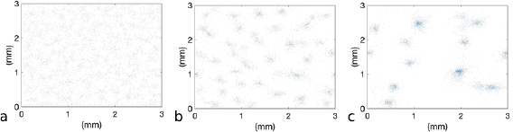
Figure B1. Depiction of one realization of the suspension at various times (a) 1 min, (b) 7 min, (c) 13 min with  in the hydrodynamic model. This value of
  represents a scenario where the bacteria are only half as sensitive to the chemical gradient resulting in a time delay in aggregate formation as well as less dense aggregates overall. Initially a uniform distribution volume fraction
  .
.
Download figure:
Standard image High-resolution imageIn figure B3(a), we see the hydrodynamic model is greatly effected by  ; namely, as
  decreases the time to reach the threshold for collective motion (volume fraction greater then. (2) greatly increases. In addition, for
  this threshold is not reached. This partially explains why the aggregates that do form are loosely held together and the local density is kept small (figure B1). The same effects are present in the pure chemotaxis model, but to a far less extent. In figure B3(b), we see that the magnitude of
  can have a large qualitative effect on aggregate formation. The general observed trend is the larger the noise the longer it takes for aggregates to form and push beyond the threshold for collective motion. Unlike the previous case, the effect of
  on the qualitative behavior is roughly the same in the pure chemotaxis and hydrodynamic models (see figure B2). In summary, the gradient sensitivity
  seems to have a great effect on the peak volume fraction, while the noise level
  effects the time until cluster formation. This is due to the fact that the noise
  makes initial aggregation formation more difficult, but once formed at a volume fraction beyond the threshold for collective motion, the hydrodynamic interactions will keep them together.
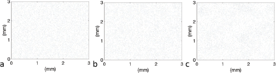
Figure B2. Depiction of one realization of the suspension at various times (a) 1 min, (b) 7 min, (c) 13 min with  in the hydrodynamic model. Here the noise is 100 times larger than figure 5 and one observes local aggregate formation is no longer present. Initially a uniform distribution volume fraction
  .
.
Download figure:
Standard image High-resolution image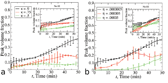
Figure B3. Peak volume fraction as a function of the (a) signal gradient sensitivity  and (b) noise in detecting the signal gradient
  . As
. As  decreases and
  increases it is hard for the cells to sense the true chemical gradient. This results in a time delay of aggregate formation or potentially the inhibition of aggregation if the values are extreme.
Download figure:
Standard image High-resolution imageAdditional simulations were run varying the model parameters estimated from the literature or could be varied based on types of bacteria; namely, the values of shape B = .9, the diffusion rate for the chemical  , the amount of chemical secreted fsec, the degradation rate for the chemical
  , and the tumbling rate
  . A summary of the results for the diffusion coefficient and diffusion scaling exponent are given in table B1. Overall, the parameter with the greatest change in the diffusive behavior of the aggregate is the shape B = 0 (spherical) versus B = .9 (ellipsoids) which led to a much larger diffusion exponent most likely due to enhanced collective swimming. In addition, the chemical diffusion coefficient
  decrease led to a diffusion coefficient of the aggregate to increase an order of magnitude. This can be explained by the fact that the chemical does not diffuse into the environment very fast leaving a chemical gradient that changes more slowly. This allows the aggregate to translate in one direction for longer periods of time and be less sensitive to small local changes. The model is not very sensitive to the other parameters in terms of the diffusion behavior of the single aggregate.
Table B1. Sensitivity of aggregate behavior to model parameters.
| Parameter Chg. | Diff. Coeff. D | Exp.  |
|---|---|---|
| Baseline |  |
1.22 |
| B = .9 |  |
1.5 |
 |
 |
1.13 |
 |
 |
1.25 |
 |
 |
1.20 |
 |
 |
1.10 |
Appendix C. High concentration regime
We briefly consider the model in the high concentration regime to illustrate how the strong fluid flow generated by the bacterium can greatly change the chemical signal distribution throughout the domain. This ultimately changes the dynamics of the suspension at large times where aggregates are forming and merging as discussed in section 4.2. Before continuing, we note the model formulation is semidilute and not designed for large bacterial volume fraction regimes as studied in this subsection. This is due to the diminished role of hydrodynamic interactions when compared with near-field excluded-volume interactions such as collisions. However, the simulations do reveal insight into the importance of the fluid-chemical signal interactions present in the hydrodynamic model (1)–(6) and noticeably absent from the pure chemotaxis model (1) and (2).
Consider figure C1 where the positions and chemical signal concentration are presented over a 6 min time frame for both approaches. In the pure chemotaxis model the bacteria secrete chemical signal at their present location and that chemical remains there for all time whereas in the hydrodynamic model the chemical signal is governed by a reaction–diffusion–advection equation (5). The principle effect of this over time is that in the high concentration regimes the bacteria begin to collectively swim forming local vortices that can attract, redistribute, and trap large concentrations of the chemical signal in locations which creates a reinforcing feedback loop. This results in densely packed aggregates capable of collectively swimming and diffusing in the domain as seen in figure 10. Without the incorporation of signal dynamics, the chemical signal concentrations are distributed locally in a small area at the location of individual cells resulting in longer time to aggregate formation and less diffusion. These results only provide minor insight into the high concentration regime and a further study with a model designed for closely-packed suspensions should be investigated to confirm these results.
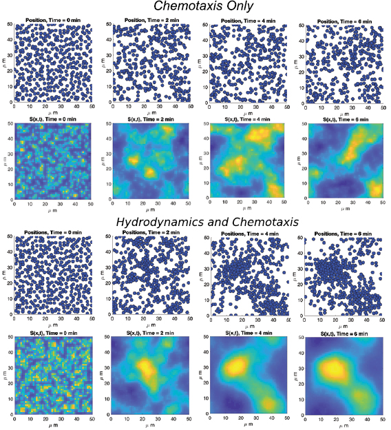
Figure C1. Comparison of chemical concentration in pure chemotaxis VJP model with the hydrodynamic model over a 6 min period in a high concentration suspension. The VJP model only includes secretion by the cells while the hydrodynamic model includes diffusion and advection of the chemical signal by the fluid. Brighter spots correspond to higher density of chemical signal. Initial bacterium volume fraction  .
.
Download figure:
Standard image High-resolution image