
Abstract
Traditionally animal groups have been characterized by the macroscopic patterns that they form. It is now recognised that such patterns convey limited information about the nature of the aggregation as a whole. Aggregate properties cannot be determined by passive observations alone; instead one must interact with them. One of the first such dynamical tests revealed that swarms of flying insects have macroscopic mechanical properties similar to solids, including a finite Young's modulus and yield strength. Here I show, somewhat counterintuitively, that the emergence of these solid-like properties can be attributed to centre-of-mass movements (heat). This suggests that perturbations can drive phase transitions.
Export citation and abstract BibTeX RIS

Original content from this work may be used under the terms of the Creative Commons Attribution 3.0 licence. Any further distribution of this work must maintain attribution to the author(s) and the title of the work, journal citation and DOI.
Introduction
Sparse swarms of flying insects show a high degree of spatial cohesion and are a form of collective animal behaviour; albeit one different from flocks and schools as they do not display ordered collective movements (Okubo 1986, Kelley and Ouellette 2013, Puckett et al 2014). Instead each individual insect moves erratically and seemingly at random within the swarm. The occurrence of these swarms makes it clear that group order and morphology are not sufficient to accurately describe animal aggregations. Indeed, it is now recognized that the properties of animal aggregates cannot be determined by passive observation alone; instead one must interact with them, by for example applying controlled perturbations (Ouellette 2017). This approach allows for the extraction of emergent group properties that are not directly linked to the characteristics of the individuals. Ni and Ouellette (2016) were the first to examine swarms of flying insects (the non-biting midge Chironomus riparius) in this way and did so by placing them under an effective load, i.e. by manipulating ground-based visual features, so-called 'swarm markers', over which swarms form. Ni and Ouellette (2016) showed that a swarm can be quasi-statically pulled apart into multiple daughter swarms which were centred over each marker once the marker separation was large enough. For intermediate separations the daughter swarms were pulled away from the centres of their respective markers and into a stable 'neck' region that linked them. This indicates that the swarms have mechanical properties similar to solids, including a finite Young's modulus and yield strength, and it shows that they lack a viscous flow regime.
Here I show how these emergent mechanical properties of insect swarms can be deduced from the simple, analytically-tractable model of Reynolds et al (2017) which is in close accord with a plethora of other (albeit passive) observations of midge swarms (Reynolds et al 2017, Reynolds 2018a, 2018b, van der Vaart et al 2019). I show that tensile strength can be attributed to the presence of centre-of-mass movements (i.e. to heat), as documented by Reynolds and Ouellette (2016). This new result along with earlier results (Reynolds et al 2017, Reynolds 2018a, 2018b, van der Vaart et al 2019) shows how the suite of observed complex, emergent, macroscopic behaviours of insect swarms (Kelley and Ouellette 2013, Ni and Ouellette 2016, Sinhuber and Ouellette 2017, van der Vaart et al 2019, Sinhuber et al 2019) can be attributed to simple processes and encapsulated within a simple model (Reynolds et al 2017, Reynolds 2018a, 2018b). This is significant because the development of accurate, generally-applicable models is of central importance, as a check on our understanding of the processes at work within swarms.
The emergence of tensile strength
In the 1D form of the model of Reynolds et al (2017) the positions, x, and velocities, u, of insects within a swarm are determined by the stochastic differential equations
where T is the velocity autocorrelation timescale,  is the velocity variance,
  is the observed swarm density profile,
  is a constant, and
  is an incremental Wiener process with correlation property
  . The first term on the right-hand side of equation (1) is a memory term that causes velocity fluctuations to relax back to their (zero) mean value. Interactions between the individuals are not explicitly modeled; rather, their net effect is subsumed in a restoring force term, since observations have suggested that to leading order insects appear to be tightly bound to the swarm itself but weakly coupled to each other inside it (Kelley and Ouellette 2013). This restoring force is given by the second term on the right-hand side of equation (1) which ensures that the spatial distribution of the simulated insects matches observations. The third term, the noise term, represents fluctuations in the resultant internal force that arise partly because of the limited number of individuals in the grouping and partly because of the nonuniformity in their spatial distribution. The model, equation (1), is effectively a first-order autoregressive stochastic process in which position and velocity are assumed to be jointly Markovian. At second-order, position, velocity and acceleration would be modelled collectively as a Markovian process. The first order model, equation (1), is appropriate because the acceleration autocorrelation timescale is shorter than the velocity autocorrelation timescale (Reynolds and Ouellette 2016). By construction, simulated trajectories have homogeneous (position-independent) Gaussian velocity statistics. When the density profile is Gaussian, as it nearly is for laboratory swarms (Kelley and Ouellette 2013), equation (1) reduces to Okubo's (1986) classic model for the simulation of insect trajectories. Similar models have also been used to model robotic swarms (Hamann and Wӧrn 2008).
In the presence of two swarm makers, swarms are bi-modal and could, for example, be characterised by
which has maxima at  . For such swarms the mean restoring force term
  . The locations of the swarm centres do, however, fluctuate over time (Ouellette and Reynolds 2016). These fluctuations can be regarded as being 'parametric' noise which operationally equates to
  . In this case the model becomes
This new model corresponds to the Fokker–Planck equation
where  is the joint distribution of velocity and position. Here equation (4) is examined in the long-time limit as
  . Here this is done following the approach of Thomson (1987) who identified the conditions under which stochastic models of tracer-particle trajectories in turbulent flows reduce to diffusion-equation models as the Lagrangian velocity-autocorrelation timescale tends to zero. In this approach the unit of time is chosen so that T is small compared with unity and the unit of length is chosen so that the size of a swarm of individuals from a point source is of order unity at times of order unity. In this system of units, velocities must be large to make up for the small timescale. Moreover, because velocities are large and rapidly changing,
  and
and  must also be large. Simple scaling arguments indicate that the long-time limit of equation (4) can be examined by replacing
  and
and  with
with  and
and  where
where  so that equation (4) becomes
If a different rescaling is adopted, then it can be shown that the dispersal is not of order unity at times of order unity. Following Thomson (1987) I now look for solutions to equation (5) that take the form  .
.
The leading order  terms give
where  is the swarm density profile predicted by the new model, equation (4).
At order 
At order 
which after integrating over all velocities becomes
i.e. becomes the non-linear diffusion equation
where from equation (7),  is the solution to
and where  . Hence the non-linear Langevin equation, equation (3), reduces to a diffusion equation in the limit
  . The density profiles are determined by equation (9) those steady-state solution is
where N is normalization constant. This theoretical prediction is supported by the results of numerical simulations using the non-linear Langevin equation, equation (3) (figure 1). A directly analogous result was obtained by Okubo (1986), albeit in a different context and for diffusion models rather than for the non-linear Langevin equation, equation (3).

Figure 1. Theoretical predictions for swarm density profiles match data from numerical simulations. The swarms are being pulled away from their respective swarm markers (dashed-lines) and displaced towards the origin. The swarms therefore appear in tension with a tensile strength that increases as centre-of-mass movements increase. Predictions (solid line) obtained from equation (12) are shown for a = 0.8, b = 0.1 and B0 = 1 with B1 = 0.1 (left), 0.3 (middle) and 0.5 (right). Simulation data (•) were obtained from equation (3) for  and T = 1.
Download figure:
Standard image High-resolution imageIn the absence of parametric noise, equation (12) rightly reduces to the unperturbed density profile,  (equation (2)). When the parametric noise,
  , is small, equation (12) has maxima close to the maxima of
  but displaced towards the origin (figure 1). And when the relative strength of the parametric noise
  there this a single maximum at the origin that becomes more pronounced as
  increases (figure 1). The swarm therefore appears to be in tension with a tensile strength that increases with increasing
  . Similarly as a pair of swarm markers are pulled apart, two daughter swarms form that are effectively pulled away from their respective markers and into the neck that links them, mirroring the observations of Ni and Ouellette (2016) (figure 2).This demonstrates that the simulated swarms, like real swarms, possess an emergent analogue of a finite Young's modulus and do not show a viscous flow regime; if they did then they would be expected to either flow back into a single swarm or to form two completely distinct swarms centred over their respective markers (Ni and Ouellette 2016). Moreover, when the marker separation becomes large enough, the model predicts that the two daughter swarms become fully distinct and that individuals no longer pass between them (figure 2). The simulated swarms like the real swarms (Ni and Ouellette 2016) therefore possess yield strengths.
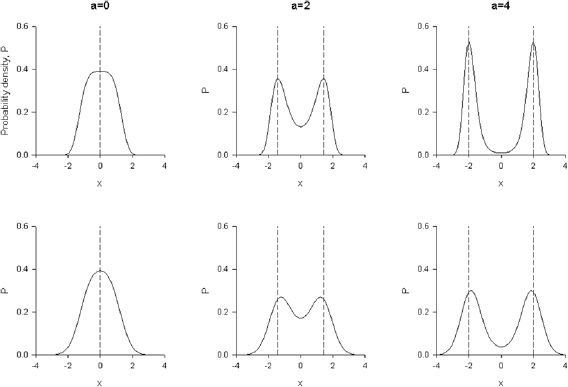
Figure 2. In the presence of parametric noise insect swarms are predicted to have an emergent analogue of a finite Young's modulus and yield stress, and do not show a viscous flow regime. When parametric noise is absent (B1 = 0) the swarm is always localized over the swarm makers ( ) (dashed lines) as it is pulled apart and so not in tension (upper panel). When parametric noise is present (B1 = 1.0) the swarm is put into tension as it is pulled apart as the swarms are being pulled away from their respective swarm markers (dashed-lines) and displaced towards the origin (lower panel) This displacement decreases with increasing separation of the swarm markers. Predictions obtained from equation (12) are shown for a = 0 (left), 2 (middle) and 4 (right), and b = 0.25.
Download figure:
Standard image High-resolution image
The results of numerical simulations (not shown) suggest that the emergence of tensile strength is a general consequence of parametric noise, arising for example when the 4th-order term rather than the 2nd-order term in the unperturbed density profile, equation (2), is noisy.
Discussion
Male midges swarm to provide a mating target for females, making stationarity desirable. Ni and Ouellette (2016) were the first to show that this biological function is reflected in an emergent physical macroscopic property of the swarm; namely its tensile strength. This emergent macroscopic mechanical property may be advantageous, in helping to stabilise insect swarms against environmental perturbations. Perturbations are inevitable in wild (natural) swarms that must contend with gusts of wind and with environmental disturbances. Here it was shown that the tensile strength of swarms can (somewhat counter-intuitively) to be attributed to centre-of-mass movements, as documented by Reynolds and Ouellette (2016) (figures 1 and 2). This may explain how these swarms possess enhanced properties relative to individual insects.
As the swarm size increases, centre-of-mass movements are determined by a balance between two competing effects: namely averaging over more but larger fluctuations because insects behave as if they are more weakly bound when in larger swarms (Kelley and Ouellette 2013). The results of preliminary numerical simulations (not shown) suggest that the latter outweighs the former and that consequently centre-of-mass movements and so tensile strength increases with increasing swarm size. Insect swarms are therefore predicted to 'solidify' as they increase in size, making it harder to pull them apart. This new prediction could be tested in the laboratory by measuring tensile strength as a function of swarm size. If true, then it suggests that insect swarms effectively cool as they increase in size. Fire ants, on the other hand, which link their bodies to form dense aggregations, behave more like viscoelastic fluids, becoming stiffer and more purely elastic as the density of the ants increases (Tennenbaum et al 2016, Vernerey et al 2018). Active changes in group morphology in response to dynamic loads are also evident in dense tree-hanging clusters of honeybees (Peleg et al 2018).
The identification and understanding of the emergent macroscopic properties of insect swarms holds promise of a unified 'thermodynamic' theory of insect swarms, where one seeks to describe their mechanical-like properties in a way that does not directly reference individual behaviours (Ouellette 2017). In such a theory different swarm morphologies and dynamics might be regarded as being different phases of insect swarming behaviour. This notion may help reconcile conflicting observations of insect swarms made in quiescent laboratory conditions and in the wild (Kelley and Ouellette 2013, Attanasi et al 2014) because, as was shown here and as was prefigured in Reynolds (2018b), perturbations may drive phase transitions.
Acknowledgments
The work at Rothamsted forms part of the smart crop protection (SCP) strategic programme (BBS/OS/CP/000001) funded through the Biotechnology and Biological Sciences Research Council's Industrial Strategy Challenge Fund. I thank Nick Ouellette, Michael Sinhuber and Kasper van der Vaart for encouraging communications.