

Abstract
We report the occurrence of bursting oscillations in a gyroscope oscillator driven by low-frequency external period forcing. The bursting patterns arise when either the frequency or amplitude of the excitation force is varied. They take the form of pulse-shaped explosions (PSEs) wherein periodic attractors of lower periodicity disappear due to the loss of asymptotic stability of the equilibrium point between resting and active states. The process involves the appearance of zero eigenvalues and the creation of new attractors of higher periodicity. Both point-cycle and cycle-cycle bursting is seen. It is accompanied by the birth of periodic attractors, ranging from period one to period four, depending on an integer n in the frequency of the parametric driving force. The dynamics of the oscillator is shown to exhibit a fold bifurcation related to critical escape transitions.
Export citation and abstract BibTeX RIS

Original content from this work may be used under the terms of the Creative Commons Attribution 4.0 licence. Any further distribution of this work must maintain attribution to the author(s) and the title of the work, journal citation and DOI.
1. Introduction
The response of nonlinear systems to various forms of external driving force has been of interest in a wide range of scientific investigations [1–8]. When the external driving force is a combination of a weak periodic signal and noise, the phenomenon of stochastic resonance [1, 2] may arise. When the noise is replaced by a high frequency field, one can realize vibrational resonance and, in this case, one of the frequencies is far higher than the other [3, 4]. However, when the two frequencies are both much less than 1 and the fast-slow dynamical characteristics still remain in the system, a phenomenon known as bursting may arise [5, 6]. This phenomenon can occur in dynamical systems whose variables evolve on two different time scales, and it has potential applications in physics [9, 10], mechanics [11], biology [12, 13], chemistry [14, 15], neuroscience [5, 6], information encoding and computation [16], and in engineering systems [17, 18]. The potential use of bursting in order to achieve extremely rapid actuators was recently demonstrated [19] in electromechanical systems .
A general mechanism underpinning the occurrence of bursting oscillations was identified and described in [20]. It is understood to arise when a dual-frequency-driven dynamical system consists of two coupled nonlinear oscillators of different frequency, where the slower oscillator sequentially switches the faster one on and off [20]. More recently, bursting has also been linked to sharp bifurcation transitions in dynamical systems [21] due to pulse-shaped explosions. Bursting involves the complex and multiple-timescale dynamics that has been receiving much attention in a diversity of dynamical system such as neuronal oscillators [5, 22], delay systems [23], biological systems with signal transduction [6, 24–26], and chemical oscillators [27]. A sharp transition behaviour, referred to as the speed escape of attractors was reported recently [28]. This transition takes attractors to infinity within a narrow interval of parameters near the critical escape (CE) condition. The result is bursting with sharp, pulse-shaped, quantitative changes appearing at the equilibrium point and limit cycle—a process referred to as a pulse-shaped explosion (PSE) [21].
Such complex bursting patterns have been investigated and reported in several classical paradigmatic oscillators including the Duffing oscillator [29], Van der Pol oscillator [30], and Mathieu-van der Pol-Duffing oscillator [31], when they are subjected to the action of two different slowly-varying sinusoidal excitations. It has also been shown that, when incommensurate fractional-order singularly perturbed Van der Pol oscillators are subjected to constant forcing, they too exhibit bursting oscillations [32, 33]. Recently, Han et al [34] reported two novel bursting patterns: turnover-of-pitchfork-hysteresis-induced bursting and compound pitchfork-hysteresis in a Duffing system with multiple excitations. The authors showed that the hysteretic behaviour between the origin and non-zero equilibria of the fast subsystem resulted from a delayed pitchfork bifurcation. Also, in [21], a novel route to bursting known as pulse-shaped explosion (PSE) was found for a paradigmatic class of nonlinear oscillators. It was shown that an equilibrium and a limit cycle can display sharp, pulse-shaped, qualitative changes as the system parameters are progressively adjusted. Very recently, Wei et al [35] analysed the route to bursting by bistable PSE in a Rayleigh oscillator with multiple slow excitations and proved that the initial phase difference of the excitations plays a significant role in transitions to different attractors and complex bursting patterns. More recently, Ma et al [31], reported the occurrence of four complicated compound bursting patterns as well as one relaxation oscillation in the Mathieu-van der Pol-Duffing.
In previous works, the focus was mostly on familiar paradigmatic models, such as the van der Pol or Duffing-like oscillators. However, there exist a variety of dual-frequency-driven nonlinear systems with broader real life, scientific and engineering applications, such as the driven gyroscope that we examine in this paper. Among its several important applications, the gyroscope functions variously as a gyrocompass, an attitude heading reference system, and an inertial measurement unit. It is used in inertial navigational aid systems. A recent review [36] comprehensively outlined and classified a wide range of commercial gyroscope applications. Supplementing the extensive body of knowledge about bursting in the literature cited above, and the references therein, we report in this paper novel bursting patterns that have not to our knowledge been described previously in relation to the driven gyroscope. This bursting is associated with the destruction of periodic attractors due to the loss in asymptotic stability of the equilibrium point separating the resting and active states, associated with the appearance of a zero eigenvalue. The process gives birth to another attractor of higher periodicity when the parametric excitation is adjusted. We analyze this new PSE bursting that occurs when a slowly-varying parametric excitation and a low frequency periodic excitation are applied to a gyroscope.
The rest of this paper is organized as follows: in section 2, we present and describe the gyroscope oscillator model to be considered together with its stability analysis. Section 3 discusses the bursting patterns. Section 4 applies the fast-slow analysis to obtain equations for the fast and slow sub-systems and describes the dynamical mechanisms underlying the bursting oscillations. Section 5 summarises our findings and conclusions.
2. Model description
The system to be considered is a driven gyroscope oscillator model [37] mounted on a vibrating base as illustrated schematically in figure 1. The equations of motion for the system dynamics when driven by either a single-frequency driving force [37], or a dual-frequency driving force [38], have been formulated using the Lagrangian approach associated with the Eulerian angles, namely, with nutation (θ), precession (ϕ) and spin (ψ). In general, the Lagrangian of the model is written as:

where I1 and I3 denote the gyroscope's polar and equatorial moments of inertia, respectively. Mg is the force due to gravity, l1 is the amplitude of the external excitation, and ω1 is the frequency of the external excitation. l2 is the amplitude of the additive external forcing at frequency ω2. ϕ and ψ are cyclic coordinates, since they do not contribute to the Lagrangian function, which provides us with two first integrals of the motion expressing the conjugate momenta. The momentum integrals are:

where ωz is the spin velocity of the gyroscope. Using the Routh's procedure and the definitions in equation (2), the Routhian of the system becomes

where the quantity A depends on the angle θ as

The system is thus treated as a single-degree-of-freedom oscillator so that its equation of motion can readily be derived from the Euler–Lagrange equation

In equation (5) F arises from all the external contributions, including the dissipative force Fd which for this model is assumed to be in linear-plus-cubic form for the model and is written as,

where D1 and D2 are positive constants. The other components of F consist of the driving forces  and
and  , as shown in figure 1. Accordingly, it is easy to show that the equation governing the gyroscope motion is given by

Redefining the variables and quantities as  ,
,  ,
,  ,
,  ,
,  and
and  , equation (7) can be rewritten in dimensionless differential equation form as

where  is a parametric driving force of amplitude a and frequency ω1.
  is an additive external periodic driving force of amplitude f and frequency ω2.
  and
and  are the linear and nonlinear cubic damping terms, respectively, with coefficients c1 and c2. Thus, the dual-frequency-driven gyroscope can be considered as a switched-system of two coupled nonlinear oscillators with different frequencies, in which the slower oscillator alternately switches the faster one on and off [20].

Figure 1. Schematic diagram of the dual-frequency-driven gyroscope.
Download figure:
Standard image High-resolution imageThe potential of equation (8) in the absence of additive driving is given by:

where 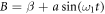 . Depending on the values of the parameters α and β, V(θ) can admit two types of potential shapes: single- and double-wells. With a = 1, c1 = 0.5, c2 = 0.05, f1 = f = 0.05, ω1 = ω = 2 and t = tn
(n = 0, 1, 2, 3,... ∞ ), V(θ) shown in figure 2 is a single-well potential and the equilibrium point of the unforced system (8) is located at the origin (
. Depending on the values of the parameters α and β, V(θ) can admit two types of potential shapes: single- and double-wells. With a = 1, c1 = 0.5, c2 = 0.05, f1 = f = 0.05, ω1 = ω = 2 and t = tn
(n = 0, 1, 2, 3,... ∞ ), V(θ) shown in figure 2 is a single-well potential and the equilibrium point of the unforced system (8) is located at the origin ( ), around which oscillatory motion of the periodically driven system (8) occurs along the principal axis of the gyroscope, which coincides with its vertical axis. Equation (8) can be expressed as two coupled autonomous differential equations, in the form

The equilibrium points of the system (10) are found by solving the system of equations:

We solve equation (11) with parameter values α = 0.1, β = −1, a = 1, c2 = 0.5, f = 0.05, ω2 = 0.01, c1 = 0.05, n = 2, and ω1 = n
ω2. We consider two cases of equilibrium points: (a) when θ1 = 0, and; (b) when θ1 has a very small value. The equilibrium point Ea,b
= (θ1, θ2) is calculated thus: when θ1 = 0, it is obvious that the equilibrium point Ea
= (0, 0) and here the system (8) is independent of the external forcing. When θ1 is very small (i.e. θ1 ≈ 0), then  and
and  . The equilibrium point therefore becomes
  . Here, the system (8) is dependent on the external forcing. It is noteworthy, then, that the equilibrium point of system (8) is affected when the external forcing acts on it (comparing Ea
and Eb
). The Jacobian matrix of the system (11) at any θ ∈ R2 is given by
. Here, the system (8) is dependent on the external forcing. It is noteworthy, then, that the equilibrium point of system (8) is affected when the external forcing acts on it (comparing Ea
and Eb
). The Jacobian matrix of the system (11) at any θ ∈ R2 is given by

where ![${K}_{1}=\left(\tfrac{3\cos {\theta }_{1}{\left[1-\cos {\theta }_{1}\right]}^{2}-\sin {\theta }_{1}[2\sin {\theta }_{1}-\sin (2{\theta }_{1})]}{{\sin }^{4}{\theta }_{1}}\right)$](https://content.cld.iop.org/journals/1402-4896/97/8/085211/revision2/psac7f98ieqn18.gif) , and
, and  and
and  .
.

Figure 2. The potential of system (8) against θ when the parameters are fixed at α = 0.1, β = −1, a = 1, c1 = 0.05, c2 = 0.5, t = 5, ω2 = 0.01, n = 2, ω1 = n ω2.
Download figure:
Standard image High-resolution imageThe stability of the equilibrium point can be obtained from the characteristic equation

From equation (13), one can deduce that, if K2 < 0 and  , Ea,b
is stable; and, if K2 > 0, then Ea,b
is unstable. This accounts for the different patterns of bifurcation that emerge as the control (i.e. the forcing amplitude a) is varied and leads to loss of stability of the equilibrium points Ea,b
. If the constant term satisfies
, Ea,b
is stable; and, if K2 > 0, then Ea,b
is unstable. This accounts for the different patterns of bifurcation that emerge as the control (i.e. the forcing amplitude a) is varied and leads to loss of stability of the equilibrium points Ea,b
. If the constant term satisfies  , fold bifurcation can take place, and jumping may occur between different equilibria. Numerically, the eigenvalues of Ja
= Ja
(Ea
) and Jb
= Jb
(Eb
) at 1.0 × 10⁴ ≤ 1 ≤ 1.15 × 10⁴ were computed and we found that they are complex conjugate eigenvalues with negative real parts. Thus, Ea
and Eb
are stable foci [39]. For example, for Ea
at t = 10000, the eigenvalues are: λ1,2 = −0.0250 ± 1.3685i; at t = 11000, the eigenvalues are: λ1,2 = −0.025 ± 0.9545i; at 11 500, the eigenvalues are: λ1,2 = −0.0250 ± 1.2710i. Also, for Ea
, at t = 10000, the eigenvalues are: λ1,2 = −0.0250 ± 1.3684i; at t = 11000, the eigenvalues are: λ1,2 = 0.0250 ± 0.9544i and finally at t = 11500, the eigenvalues are: λ1,2 = −0.0250 ± 1.2710i.
, fold bifurcation can take place, and jumping may occur between different equilibria. Numerically, the eigenvalues of Ja
= Ja
(Ea
) and Jb
= Jb
(Eb
) at 1.0 × 10⁴ ≤ 1 ≤ 1.15 × 10⁴ were computed and we found that they are complex conjugate eigenvalues with negative real parts. Thus, Ea
and Eb
are stable foci [39]. For example, for Ea
at t = 10000, the eigenvalues are: λ1,2 = −0.0250 ± 1.3685i; at t = 11000, the eigenvalues are: λ1,2 = −0.025 ± 0.9545i; at 11 500, the eigenvalues are: λ1,2 = −0.0250 ± 1.2710i. Also, for Ea
, at t = 10000, the eigenvalues are: λ1,2 = −0.0250 ± 1.3684i; at t = 11000, the eigenvalues are: λ1,2 = 0.0250 ± 0.9544i and finally at t = 11500, the eigenvalues are: λ1,2 = −0.0250 ± 1.2710i.
Now, in the absence of the additive external periodic forcing  , the system (8), or its equivalent autonomous version given by equation (10), exhibit some interesting dynamical features. Here, we illustrate the basic dynamical properties using, for instance, the one-parameter bifurcation diagrams and the corresponding Lyapunov exponent (LE) spectrum as functions of the amplitude a with the corresponding phase space structures and Poincaré section in selected regimes as shown in figure 3. The bifurcation structure in figure 3(a) was investigated earlier by Chen [37]. The bifurcation diagram and the corresponding Lyapunov exponent (LE) spectrum in the regime of interest capture all the essential features in figure 3(a), setting α = 10, β = 1, c1 = 0.5, c2 = 0.005, and Ω = 2. Note that in [37], the upper wing bifurcation sequence shown in figure 3 was reported. However, Dooren [40] conjectured that, by starting with a different set of initial conditions, a second bifurcation sequence, occurring in the lower wing can be obtained. Thus, the upper and lower wing bifurcation cascades when combined gives the complete bifurcation structure of the system as a function of the amplitude a—the lower sequence coexisting with the upper one. The simulations in both papers show the manifestation of extreme sensitivity to initial conditions which is a hallmark of nonlinear systems as well as indicating the existence of hidden attractors. In figure 3, we display the complete bifurcation structure using forward and backward propagations of the amplitude a without intentional change in the variable's initial conditions. In forward propagation, the amplitude was increased such that a = a + δ
a whereas in backward propagation, the amplitude was decreased such that a = a − δ
a, where δ
a is the increment or decrement in a. This approach is effective in capturing the salient features and the entire sequence of bifurcations, including all the hidden attractors.
, the system (8), or its equivalent autonomous version given by equation (10), exhibit some interesting dynamical features. Here, we illustrate the basic dynamical properties using, for instance, the one-parameter bifurcation diagrams and the corresponding Lyapunov exponent (LE) spectrum as functions of the amplitude a with the corresponding phase space structures and Poincaré section in selected regimes as shown in figure 3. The bifurcation structure in figure 3(a) was investigated earlier by Chen [37]. The bifurcation diagram and the corresponding Lyapunov exponent (LE) spectrum in the regime of interest capture all the essential features in figure 3(a), setting α = 10, β = 1, c1 = 0.5, c2 = 0.005, and Ω = 2. Note that in [37], the upper wing bifurcation sequence shown in figure 3 was reported. However, Dooren [40] conjectured that, by starting with a different set of initial conditions, a second bifurcation sequence, occurring in the lower wing can be obtained. Thus, the upper and lower wing bifurcation cascades when combined gives the complete bifurcation structure of the system as a function of the amplitude a—the lower sequence coexisting with the upper one. The simulations in both papers show the manifestation of extreme sensitivity to initial conditions which is a hallmark of nonlinear systems as well as indicating the existence of hidden attractors. In figure 3, we display the complete bifurcation structure using forward and backward propagations of the amplitude a without intentional change in the variable's initial conditions. In forward propagation, the amplitude was increased such that a = a + δ
a whereas in backward propagation, the amplitude was decreased such that a = a − δ
a, where δ
a is the increment or decrement in a. This approach is effective in capturing the salient features and the entire sequence of bifurcations, including all the hidden attractors.

Figure 3. (a) One-parameter bifurcation diagram computed based on forward (blue colour) and backward (red colour) propagations and the corresponding Lyapunov (λ) exponents spectrum (green colour) illustrating the period-doubling cascades to chaos. Subplots (b) Periodic two attractor for a = 32.0 and (c) Chaotic attractor for a = 35.5. In (b) the red and blue lines represent the trajectories of the upper and lower wing attractors, with their corresponding Poincaré points shown as open and closed black points. The other parameters are: α = 10, β = 1.0, c1 = 0.5, c2 = 0.005, and ω1 = 2.0.
Download figure:
Standard image High-resolution imageIn addition, the images in figure 3 have certain features that are typical of damped-driven systems such as the Duffing oscillator and pendulum reported by Szemplińska-Stupnicka and Tyrkiel [41] and Parlitz [42] and by many others. Specifically, prior to the critical period-doubling bifurcation point at a = acr , where acr ≈ 32.9, there are two coexisting resonant periodic attractors within a broad range of driving amplitudes a, located in the upper and lower wings of the bifurcation curve [figure 3(b)]. When a ≥ ac the period-doubling cascade continues and terminates in the stable chaotic domain occurring in the neighbourhood of 34.7 < a < 36.2 [figure 3(c)].
In the presence of the additive external periodic driving force  the system (8) exhibited the phenomenon of vibrational resonance, when one of the frequencies is much larger than the other, i.e. ω2 ≫ ω1 or ω1 ≫ ω2, as reported in our recent paper [38]. Under these conditions, we showed that the response of the driven gyroscope to the low frequency force can be optimised by the presence and properties of the high-frequency component. In the present paper, we consider a different scenario where the frequencies ω1 and ω2 are such that ω1 = n
ω2, i.e. commensurate frequencies—n being a positive integer [43]. In general, ω1,2 ≪ 1 indicates the slowly-varying excitations which are a requirement for the occurrence of bursting [29, 30]. Consequently, the system (parametric excitation) changes n-times while the external inertia force changes once per revolution. Parameter values in this study are taken as α = 0.1; β = − 1; a = 1; c2 = 0.5; f = 0.05; ω2 = 0.01 and c1 = 0.05. Remarkably, the bursting phenomenon associated with system (8) is different from the phenomenon of parametric vibrational resonance exhibited by this gyroscope model driven by dual frequency forces ω1 and ω2, such that ω1 ≫ ω2 or ω2 ≫ ω1.
the system (8) exhibited the phenomenon of vibrational resonance, when one of the frequencies is much larger than the other, i.e. ω2 ≫ ω1 or ω1 ≫ ω2, as reported in our recent paper [38]. Under these conditions, we showed that the response of the driven gyroscope to the low frequency force can be optimised by the presence and properties of the high-frequency component. In the present paper, we consider a different scenario where the frequencies ω1 and ω2 are such that ω1 = n
ω2, i.e. commensurate frequencies—n being a positive integer [43]. In general, ω1,2 ≪ 1 indicates the slowly-varying excitations which are a requirement for the occurrence of bursting [29, 30]. Consequently, the system (parametric excitation) changes n-times while the external inertia force changes once per revolution. Parameter values in this study are taken as α = 0.1; β = − 1; a = 1; c2 = 0.5; f = 0.05; ω2 = 0.01 and c1 = 0.05. Remarkably, the bursting phenomenon associated with system (8) is different from the phenomenon of parametric vibrational resonance exhibited by this gyroscope model driven by dual frequency forces ω1 and ω2, such that ω1 ≫ ω2 or ω2 ≫ ω1.
The simulations are carried out with initial conditions θ1(0) = 0.1, θ2(0) = 0.2 (the initial condition is shown by the black circle in figures 4(b), 5(b), 6(b) and 8(b)).

Figure 4. (a) Typical bursting pattern, and; (b) plot of trajectories in the phase plane ( ) of the system (8) with n = 2. The other parameters fixed at α = 0.1, β = −1, a = 1, c2 = 0.5, f = 0.05, ω2 = 0.01, c1 = 0.05.
Download figure:
Standard image High-resolution image3. Bursting patterns
In order to provide a clear understanding of bursting phenomenon, we discuss several cases of bursting for different values of n. In general, bursting appears for all integer values of n; however the bursting dynamics for odd integer values is not distinct and bears no relation to the system's periodicity. Thus, we focus mainly on the occurrence of bursting for even integer values of n. We first discuss a case when n = 2. Figure 4(a) shows a single peak pulse-shaped explosion (PSE) when the other parameters are fixed as stated earlier. It is called a single PSE because the peak values of θ (up state and down state) have the same magnitude. It is similar to periodic spiking in that its response to perturbation produces a single spike at a time [24]. The quiescent state is the rest state in-between the spikes; however, it is characterized by a periodic attractor of period one, as seen in figure 4(b).
When the quiescent state is an equilibrium point and the spiking state is a limit cycle, the bursting type is called point-cycle bursting [24]; but if the quiescent state is a small amplitude (sub-threshold) oscillation, then it is called cycle-cycle bursting [24]. Due to the unstable quiescent state in cycle-cycle bursting, the fast variable requires some time (i.e. slow passage) to diverge from the equilibrium. The slow passage can be shortened by noise or weak input from other bursters, which provides a useful mechanism for instantaneous synchronization of bursters whereby small perturbations from the other burster can cause an instant transition to the active state even when they have essentially different interburst frequencies [24].
3.1. Bursting oscillation patterns with n > 2
We now consider higher values of n (i.e. n > 2). Figures 5–8 show that, with n ≥ 4, a number of bursting pattern containing multiple clusters can be observed in each cycle of bursting. Figure 5(a) has a few threshold oscillations of diminishing amplitude in the quiescent state and, unlike figure 4(a), the spike has two peaks PSEs. This implies that the value of n impacts on the number of peak PSEs that can occur. Notably, the bursting pattern observed for n = 4 is a period two orbit bursting as indicated in the phase trajectory shown in figure 5(b). Thus, we point out that the PSE bursting noticed here is associated with period-doubling bifurcation sequences. For example, the period one attractor observed in figure 4 when n = 2 undergoes a period-doubling bifurcation and gives birth to new attractor of period two. Furthermore, we examined the bursting pattern when n = 8. The result is shown in figure 6(a). In this case, the bursting pattern is characterised by more threshold oscillations in the quiescent state than found figure 5(a) as well as more peak PSEs. In addition, we find the emergence of a period three orbit in the phase space as shown in figure 6(b). Such a scenario is connected with a crisis-like bifurcation in which an attractor collides with its basin boundaries and loses stability during the collision process—consequently, a new attractor of different orbit is created. Indeed, as the value of the integer n increases the bursting pattern becomes more complex with increased periodicity. With n = 10, as shown in figure 7(a), the threshold oscillations in the quiescent state is more pronounced than when n = 8 and a period four bursting is depicted in figure 6(b). Hence, as the integer n increases, the periodicity of the newly-created attractors increases. We therefore conjecture that, as the integer n of excitation varies progressively, parametrically excited systems subjected to two commensurate frequencies transit from one periodic state to another. Figures 6(a) and 7(a) depict a total cycle-cycle bursting with small amplitude oscillation.

Figure 5. (a) Bursting pattern, and; (b) plot of trajectories in the phase plane ( ) of the system (8) with n = 4. The other parameters fixed at α = 0.1, β = −1, a = 1, c2 = 0.5, f = 0.05, ω2 = 0.01, c1 = 0.05.
Download figure:
Standard image High-resolution image
Figure 6. (a) Bursting pattern, and; (b) plot of trajectories in the phase plane ( ) of system (8) with n = 8. The other parameters fixed at α = 0.1; β = − 1; a = 1; c2 = 0.5; f = 0.05; ω2 = 0.01; c1 = 0.05.
Download figure:
Standard image High-resolution image
Figure 7. (a) Bursting pattern, and; (b) plot of trajectories in the phase plane ( ) of system (8) with n = 10. The other parameters fixed at α = 0.1; β = − 1; a = 1; c2 = 0.5; f = 0.05; ω2 = 0.01; c1 = 0.05.
Download figure:
Standard image High-resolution image3.2. Impact of excitation amplitude
We now focus on the effect of the excitation amplitude on the bursting dynamics. First, we consider the effect of the parametric excitation amplitude a on the bursting pattern. It can be seen in figure 8(a) that, when a = 2 and the other parameters are taken as in figure 4, a new bursting oscillation pattern is formed. It is a complex bursting pattern, similar to that described in [43]. However, the bursting observed in [43] was due to two incommensurate excitation frequencies whereas, in the present paper, the bursting patterns observed are associated with commensurate frequencies. Comparing figures 4(a) and 8(a), it can be seen that the spikes (up and down) in figure 8(a) are characterized by rough edges, unlike figure 4(a) in which spikes have sharp edges. It can be concluded that the amplitude a of the parametric excitation affects the reversal period (sharp/delayed) of the spikes in the bursting pattern. The latter persists for other values of a (i.e. for a ≥ 4). Figures 8(b)–(c) display complex bursting patterns showing a decrease in the complexity of the threshold oscillations as the value of a increases. Here, the complexity of the oscillations in the up state, the down state and the quiescent state decreases as the value of a increases.

Figure 8. Complex bursting pattern in system (8) with the following parameters: (a) a = 2, (b) a = 4, (c) a = 8 and (d) a = 15. The other parameters fixed at α = 0.1, β = −1, c2 = 0.5, f = 0.05, ω2 = 0.01, n = 2, c1 = 0.05.
Download figure:
Standard image High-resolution imageAlso, considering equation (9), it can be seen that the potential of system (8) depends on the parametric excitation amplitude, a. Figure 9 shows the impact of variations in a on the system's potential structure. When a is taken as a = 1, 2, 4 or 8, it displays a single-well potential with its local minimum at θ = 0; whereas when a = 15, the potential is a double-well potential with its local maximum at θ = 0 and two local minima located at θ = ±2.6 around which oscillatory motion takes place.
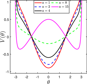
Figure 9. The potential of system (8)against θ with different values of a. Other parameters are fixed as follows: α = 0.1, β = −1, n = 2, c1 = 0.05, c2 = 0.5,t = 5, ω2 = 0.01, ω1 = n ω2.
Download figure:
Standard image High-resolution imageNext, considering the impact of the external driving force amplitude f, figure 10(a) shows the bursting pattern formed when f is increased to 0.1 with the other parameters still fixed as in figure 4. The diminishing amplitude threshold oscillation in the quiescent state is similar to those shown in figure 4, while the spikes in the up state and down state occur with rough edges. This implies that after the perturbation, the reverse mode of the system will not be as sharp as in figure 4 but will occur with some intermittent delays. Figures 10(b), (c) show that as the value of f increases, the time taken for the up state and the down state to reverse increases. In practice, the appearance of either a sharp reverse mode or a delayed reverse mode can be effected by adjusting the value of f to yield the desired result.

Figure 10. Complex bursting pattern in system (8) for different values of the amplitude f: (a) f = 0.1, (b) f = 0.2, (c) f = 0.3, and (d) f = 0.4. The other parameters were fixed as follows: α = 0.1, β = −1, n = 2, c2 = 0.5, a = 1, ω2 = 0.01, c1 = 0.05.
Download figure:
Standard image High-resolution image4. Fast-slow and bifurcation analysis
4.1. Fast-slow analysis
Equation (8) describes a fast–slow system with two slow excitations (0 < ω1,2 ≪ 1). It is when a system exhibits fast-slow dynamics that bursting oscillations may occur. In system (8) the parametric excitation provides the fast dynamics while the external forcing is taken as the slow dynamics, with the two commensurate frequencies ω1 and ω2 related by ω1 = n ω2. Therefore, we obtain the transformed fast-slow system as

where

is the only slow variable of the system. Based on De Moivre's theorem, the trigonometric polynomial function,  , resulting from
  is
is

where m(m ≤ n) is the maximum odd number not larger than n and i is a complex number. Substituting the slow variable ψ(t) in equation (14) leads to a fast subsystem, given as

where  is the control parameter.
In order to establish the transition condition, we examine the behaviour of the fast subsystem. If  , the fast subsystem has two equilibrium points, (θ1, θ2), where θi
, (i = 1, 2) is determined from the real roots of
, the fast subsystem has two equilibrium points, (θ1, θ2), where θi
, (i = 1, 2) is determined from the real roots of

For simplicity, we assume that θ is small and as a and χ approach the critical escape (CE) condition  i.e.
i.e.  , the equilibrium will tend to infinity. Hence, at the CE condition, equilibrium does not exist. Noting that β = −1 in our computations, the CE condition becomes
  . This condition shall be explored later while examining the PSE associated with the equilibrium points.
4.2. Bifurcation analysis
When a system's trajectory transits between attractors, bursting can be created. Consequently, bursting can be obtained in the system (8) when the trajectory transits between the different attractors and the dynamical mechanism of bursting patterns shown in figures 4–7 can then be analysed. Recall that bursting is a complex oscillation, where the trajectory undergoes transitions between an active state of rapid spike oscillations and a state of quiescence; the dynamical mechanism (bifurcation) underlying the process can be explored.
Based on the transition condition obtained earlier, we now examine the PSE associated with the equilibrium points by analysing the bifurcation of system 8 s a function of χ with different values of n (say n = 2, 4, 8 and 10), exploring the PSE related to equilibrium. We start with the bifurcation behaviour when n = 2. Figure 11(a) shows the bifurcation behaviour of the fast subsystem for n = 2 which exhibits two critical escapes (CE) lines at CE1 = (−0.73,0) and CE 2 = (0.73, 0) where a fold bifurcation related to CE transitions takes place. As the slow variable, χ, increases from −1, −0.4 where a large-amplitude oscillation takes place. It then switches to a rest state between −0.4 ≤ χ ≤ 0.4, after which it switches to an active regime between 0.4 ≤ χ ≤ 0.9,and finally comes to a rest state between 0.9 ≤ χ ≤ 1 through small-amplitude oscillations.

Figure 11. One parameter bifurcation of the variable θ as function of χ for system (8) with control parameter χ for different values of n: (a) n = 2, (b) n = 4, (c) n = 8 and (d) n = 10. The other parameters were fixed as follows: α = 0.1, β = −1, a = 1, c2 = 0.5, f = 0.05, ω2 = 0.01, c1 = 0.05.
Download figure:
Standard image High-resolution imageFor other values of n (i.e. n = 4, 8 and 10), figures 11(b)–(d) depicts the bifurcation behaviour of the fast subsystem as a function of the control parameter, χ. PSEs showing more than two peaks can be observed in the fast subsystem with n ≥ 4. When n = 4 the bifurcation behaviour of the fast subsystem exhibits four CE lines at CE1 = (−0.9, 0), CE2 = (−0.45, 0), CE 3 = (0.45, 0) and CE 4 = (0.9, 0) as shown in figure 11(b), where a fold bifurcation related to CE transitions takes place. Between −1 ≤ χ ≤ −0.85, the dynamics is in an active regime with appreciably high-amplitude oscillation. The rest state with small-amplitude oscillations follows between −0.85 ≤ χ ≤ −0.55. It then switches to an active domain between −0.55 ≤ χ ≤ −0.3 before entering a quieter rest state between −0.3 ≤ χ ≤ 0.3. The active regime between 0.3 ≤ χ ≤ 0.55 is followed by a small-amplitude quiescent state between 0.55 ≤ χ ≤ 0.85 and finally switches to an active regime between 0.85 ≤ χ ≤ 1. Figure 11(c) displays six CE lines at CE1 = (−0.95, 0), CE2 = (−0.85, 0), CE3 = (−0.5, 0), CE 4 = (0.5, 0), CE 5 = (0.85, 0) and CE 6 = (0.95, 0) with n = 8. The rest states in-between the active regimes exhibit small-amplitude oscillations. Figure 11(d) shows a fold bifurcation related to CE transitions with n = 10 having eight CE lines at CE1 = (−1, 0), CE2 = (−0.85, 0), CE3 = (−0.75,0), CE4 = (−0.4, 0), CE 5 = (0.4, 0), CE 6 = (0.75, 0), CE 7 = (0.85, 0) and CE 8 = (1, 0) and every rest state exhibits small-amplitude oscillations. Obviously, the system (8) displays stability within − 1 ≤ χ ≤ 1 which connotes a stable PSE of the equilibrium attractor.
Finally, we examine the mechanism of bursting by analyzing the stability of the fast subsystem given by Eqn (17). The equilibrium point of the fast subsystem can be written in the form (θ1, θ2), where θ2 = 0 and θ1 is determined by the real roots of equation (18). Linearization of the fast subsystem at the equilibrium points (θ1, θ2) leads to the Jacobian matrix

where

 and
and  . From equation (19), we obtain the characteristic equation as

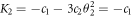
The equilibrium point is stable if K2 < 0 and 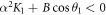 , and unstable if K2 > 0. For the set of parameters values used in the numerical simulations,
  and K2 < 0. In addition, the condition
  is never satisfied. Hence, the equilibrium point is never at infinity. We found that the transition between the rest state and active state is associated with the appearance of a zero eigenvalue of the characteristic equation when
  . That is, the asymptotic stability of the equilibrium point is lost when a transition occurs between the rest and active states. The active state exists between the critical values of χ, where
  and are shown in the shaded regions of figure 12(a) and 13(a).

Figure 12. Fast-slow analysis for the case n = 2. (a) Overlay of the bifurcation diagram of the equilibrium point θ with respect to the control parameter χ (thick blue curve) and the transformed phase diagram in the plane (χ, θ) (dashed black curve). (b) Time series of θ(t) (thick black curve) overlaid with χ as a function of t (dashed red curve).
Download figure:
Standard image High-resolution imageWe now discuss the transition mechanism for the two cases as illustrated in figures 12(a) and 13(a), where we show the superposition of the bifurcation diagram of the equilibrium point θ with respect to the control parameter χ and the transformed phase diagram in the (χ, θ) plane. First, let us consider the Periodic-One bursting reported for n = 2 and illustrated in figure 4. Figure 12(a) shows that, as χ changes from −1 to +1, a zero eigenvalue appears for a broad range of χ values and a transition to the active state takes place in the region spanning 0.63 ≤ χ ≤ 0.79 (denoted as Region 1). Figure 12(a) shows that as θ starts from a near zero negative value, it becomes positive as it crosses χ = 0 values. However, as χ approaches Region 1 in the neighbourhood of χ = 0.63, the equilibrium point increases sharply with the appearance of an active state, reaching a maximum at χ = 0.63. Evidently, there is a decrease in the equilibrium point to a local minimum at χ = 0.71 and an increase to the maximum value as χ approaches 0.79. Moreover, as χ leaves Region 1, there is a sharp decrease in the equilibrium point as the system undergoes a transition from the active state to the rest state. From figure 12(a), the transformed phase diagram shows that the transition to the active state from the rest state occurs within Region 1. Note that, due to the trigonometric nature of the control parameter, χ, for every region where there is a transition between the rest and active states, there is another transition region on the other side of the χ = 0 line. That is, for a transition in the Region 1 between 0.63 ≤ χ ≤ 0.79, there is a corresponding transition due to Region 1 also between −0.63 ≥ χ ≥ −0.79, herein denoted as Region 2 in figure 12(b). These observations from figure 12(a) are further corroborated in figure 12(b). In figure 12(b), we display the time series θ(t), overlaid with the χ as a function of t. The transition region with 0.63 ≤ χ ≤ 0.79 (the up state) and −0.63 ≥ χ ≥ −0.79 (the down state) as predicted from figure 12(a) are indicated. It can be seen that the transition to the active state occurs when χ values coincide with the aforementioned transition regions. The up state occur at χ values lying between 0.63 ≤ χ ≤ 0.79 and the down state occurs at χ values between −0.63 ≥ χ ≥ -0.79.
For n = 4 where Period-Two bursting was found in figures 5, 13(a) shows that the transition to the active state occurs within the regions labelled Region 1 (−0.90 ≥ χ ≥ −0.95) and Region 2 (0.35 ≤ χ ≤ 0.42). In addition, there exist two transition regions located within 0.90 ≤ χ ≤ 0.95 and −0.35 ≥ χ ≥ −0.42 - corresponding to Region 1 and Region 2, respectively. There are an additional two regimes denoted as Regions 3 and Regions 4. Hence, as χ increases from −1 to +1, there are four transition regimes from rest state to active state. Figure 13(b) shows the time series θ(t) overlaid with the χ as a function of t for n = 4, in which the four transition regions are clearly indicated. Again, the transition to the active state occurs when χ values are chosen within the transition regions. The up states occur in the interval 0.35 ≤ χ ≤ 0.42 and 0.90 ≤ χ ≤ 0.95, while the down states occur in the neighborhood of −0.35 ≥ χ ≥ −0.42 and −0.90 ≥ χ ≥ −0.95. In general, for any n = 2, 4, 6, ..., there are 2n transition regions as χ switches between its peak values from −1 to +1. Moreover, the large amplitude oscillations created as the system moves from the rest state to active states within the transition regions are induced by the loss of asymptotic stability due to the appearance of a zero eigenvalue of the equilibrium point when  .
.

Figure 13. Fast-slow analysis for the case n = 4. (a) Overlay of the bifurcation diagram of the equilibrium point θ with respect to the control parameter χ (thick blue curve) and the transformed phase diagram in the plane (χ, θ) (dashed black curve). (b) Time series of θ(t) (thick black curve) overlaid with χ as a function of t (dashed red curve).
Download figure:
Standard image High-resolution image
5. Summary and concluding remarks
We have examined the occurrence of bursting oscillations in a gyroscope oscillator subjected to a low frequency external driving force and a low frequency parametric excitation force. The oscillation observed exhibits a PSE pulse-shaped bursting pattern with changing bursting periods as the frequency of the parametric excitation is progressively varied. A change in the amplitude of the parametric excitations, as well as a change in the amplitude of the external forcing, affects this bursting pattern. The bifurcation diagram of the fast subsystem was found to exhibit different numbers of CE lines where fold bifurcations related to CE transitions take place. In general, the bursting patterns found in this model arise from losses in the asymptotic stability of equilibrium point between the rest and active states associated with the appearance of zero eigenvalue. Understanding the bursting oscillations pattern in the gyroscope oscillator could be useful in its application to micro-electromechanical systems (MEMS) gyroscopes with multiple driving forces [44, 45] where the phenomenon can be employed to achieve rapid movement and control [19]. These can readily be explored in control systems and devices such as: RF switches; a phase shifter for spacecraft communication; lab-on-a-chip microsensors for remote chemical detection; compact thermal control systems for pico- and nano-satellites and inertial sensors for spacecraft navigation, which are all products of MEMS technology [46].
Acknowledgments
We are grateful for support from the Engineering and Physical Sciences Research Council (United Kingdom) under research Grant No. EP/P022197/1.
Data availability statement
No new data were created or analysed in this study.