


Abstract
We provide an updated study of some electronic properties of graphene nanoscrolls, exploiting a related curved space Dirac equation for the charge carriers. To this end, we consider an explicit parametrization in cylindrical coordinates, together with analytical solutions for the pseudoparticle modes living on the two–dimensional background. These results are then used to obtain a compact expression for the sample optical conductivity, deriving from a Kubo formula adapted to the 1 + 2 dimensional curved space. The latter formulation is then adopted to perform some simulations for a cylindrical nanoscroll geometry.
1. Introduction
The discovery of graphene–like materials has determined a great interest deriving form the synthesis of real, prototypical two–dimensional systems [1, 2]. Graphene, in particular, has emerged as an exciting framework with notable physical properties [3–6].
A graphene layer consists in a single–atom–thick sheet of hexagonally arrayed carbon atoms. It has attracted attention because of its electronic, mechanical and optical characteristics [7–9] together with a variety of quantum phenomena that are characteristic of 2D Dirac fermions, such as specific integer and fractional quantum Hall effects or peculiar oscillations exhibiting non–zero Berry's phase [10–16]. All these properties, combined with its stability, flexibility and near-ballistic transport at room temperature, make graphene an ideal material for many nanoscale applications [4, 17–21].
The substrate electronic properties are naturally described in terms of charge carriers that, near the Fermi energy, mimic particles with zero mass and an effective limiting speed. It is then possible to observe a relativistic–like particle motion at sub-luminal velocities [3, 7, 22]. We then find the equivalent of a 2D gas of charged particles described by a relativistic Dirac equation, rather than a non-relativistic Schrödinger equation with an effective mass. The particle zero–mass description is a robust feature of graphene, being protected, by a certain extent, from the presence of time–reversal and parity symmetry of the system. The introduction of electron-electron interactions or substrate distortions turn out to be quite irrelevant at low energies, and do not alter the massless formulation [23–26].
From the perspective of high energy physics, the existence of observable pseudoparticles moving in a real, curved background is of great interest. The first remarkable consequence is the possibility to examine quantum fields living in a laboratory system which acts as a lower–dimensional curved spacetime [5, 8, 27, 28]. This provides a bridge between condensed matter and theoretical quantum models, where the analogues of many high energy physics effects can be explored in a solid state system [7, 9, 22, 29–34]. Moreover, the massless pseudoparticle motion realizes the analog of a relativistic system, with characteristic limiting velocity given by the Fermi velocity vF rather than the speed of light c. 1 Then, one is naturally led to consider this special relativistic–like behaviour combined with a supporting curved geometric background, the latter obtained by geometrically deforming the graphene layer. This would give rise to a tabletop general relativistic–like system, the charge carriers acting as Dirac pseudoparticles in a lower–dimensional curved spacetime [9, 27, 30, 34–46]. This unique combination therefore offers the possibility of observing quantum fields in a real, curved background, giving rise to many peculiar effects affecting the electronic properties of the substrate. The study of 2D Dirac materials could then provide new insights in theoretical as well as in experimental physics.
Another fascinating opportunity would be to exploit the general relativistic nature of a geometrically deformed layer to test some quantum gravity scenarios [47–49]. This approach is dubbed bottom–up formulation, and considers suitable condensed matter system as supporting frameworks in which to observe analogues of gravitational effects. The sine qua non of any 'analogue model' is, in particular, the existence of some emerging effective metric that captures the notion of curved spacetime arising in general relativity [48, 49]: the latter effective metric controls the dynamics of quantum particles, and it is then possible to exploit some convenient techniques usually belonging to general relativity (or quantum gravity). On the other hand, there is the possibility that direct observation of unexpected or unconventional effects could, in some cases, lead to suitable variants of these analogue models, which would in turn provide some hints towards new (or more complete) formulations of quantum gravity theories in high energy physics.
In the following, we will not address issues related to quantum gravity models. We will instead take advantage of the described analogue–gravity approach to investigate some physical features of specific curved configurations for a graphene–like substrate, using the related effective metric to study the pseudoparticle motion. 2 In particular, we will focus on graphene nanoscrolls optical properties, exploiting a curved space formulation that, in turn, gives rise to a Dirac equation in cylindrical geometry. The latter can be used to describe the dynamics of the fermionic charge carriers, and will be instrumental in determining a simple, explicit form of an adapted Kubo formula for the sample optical conductivity.
2. Dirac formalism
The hypothesis that carbon–based materials may realize the physics of massless Dirac fields dates back to the 1980s [53], a property that discriminates graphene from other bidimensional systems and makes it a privileged framework for theoretical investigations and experimental applications.
The origin of the Dirac formulation in graphene is different from the one in high energy physics. 3 The spinorial nature of the fields in graphene–like materials emerges as a consequence of the lattice topological structure. In the honeycomb lattice, a unit cell is composed of two adjacent atoms belonging to the two inequivalent, interpenetrating triangular sublattices giving rise to the global hexagonal geometry. The same structure is present in the reciprocal momentum space and reflects in the single–electron wavefunction. The latter is conveniently expressed as a two–component spinor, satisfying a 2D Dirac Hamiltonian describing massless fermions [3, 6, 22], the characterization being not affected by lattice deformations retaining the topological configuration [7, 26].
Electronic structure. The graphene honeycomb crystal structure is characterized by two types of C-C bonds (denoted by σ, π) constructed from the four valence orbitals. In particular, three in–plane σ bonds join every C atom to its three neighbours. An additional type of bond is associated with the overlap of out–of–plane π orbitals (or pz orbitals, z being the direction perpendicular to the sheet). In general, one expects the electronic wavefunctions from different lattice atoms to overlap. However, there is no overlap between the pz orbitals and the s, px , py orbitals involved in the σ bonds. Consequently, the pz electrons, which form the π bands in graphene, can be treated independently from the other valence electrons [54].
The pseudorelativistic characterization of the pz charge carriers is manifest in the reciprocal momentum space, where the energy turns out to be a linear function of the quasi-momentum at the vertices of the first Brillouin zone (FBZ). The latter, in its turn, has an hexagonal structure, rotated by a π/2 angle with respect to the honeycomb lattice. The six corners of the FBZ hexagons are subdivided into two inequivalent classes, since only two are truly independent, while the other four can be reached by means of a reciprocal lattice vector. The mentioned vertices of the hexagonal FBZ are referred to as Dirac points.
The substrate intrinsic Fermi surface is reduced to the six Dirac points of the FBZ, where the π band electronic dispersion is found to be linear, like in relativistic massless particles. This is in contrast with the usual, quadratic energy-momentum relation obeyed by electrons at band edges in conventional semiconductors. Graphene turns then out to be a special semimetal (zero–gap semiconductor), featuring massless Dirac charge carriers with relativistic–like behaviour with respect to vF. In particular, three–dimensional plots of the two–dimensional linear bands produce Dirac cones, whose conical apices touch at the FBZ corners. The Fermi level is then taken as the zero–energy reference, and the Fermi surface is defined by means of the Dirac points. Since only the bonding π states lie in the vicinity of the Fermi level, the σ bonds are usually neglected in the calculations of the electronic properties of graphene around the Fermi energy. 4 The electronic properties are then determined by the π orbitals, which give rise to wide electronic valence and conduction bands. Within the discussed approximation, it is then easy to describe the electronic spectrum of single–layer graphene in terms of a rather simple tight–binding Hamiltonian, leading to analytical solutions for their eigenstates [43, 55]. 5
When a graphene sheet is bent, the bond angles between the σ and π orbitals varies, introducing peculiar curvature effects into the electronic properties of the material. We will analyse this occurrence more in detail in the following sections.
Continuum limit. Graphene can be warped in the out–of–plane direction, similar to a sheet of paper [56, 57]. The electronic structure of graphene is directly affected by curvature [58], the specific folding inducing various and intriguing physical effects. The analysis of certain curved configurations can bring out some peculiar features of the pseudoparticles, originating from the discussed massless behaviour in the curved substrate [59–62]. A suitable choice of the sample geometry and related parametrization would give rise to some remarkable (and detectable) physical properties.
The quantum Dirac formulation is fully realized for the quasiparticles when restricting to low–energy excitations: for energy regimes well below Eℓ ∼ vF/ℓ, the charge carriers wavelength is large with respect to the lattice average parameter ℓ ∼ 0.142 nm, so that the pseudoparticles do not perceive the discrete layer nature, then justifying the continuum picture.
Furthermore, electrons featuring very large wavelengths are more susceptible to substrate (spacetime) curvature, again suggesting to limit ourselves to low–energy ranges, where the quasiparticles wavelengths are large if compared with the honeycomb dimensions,

Finally, we should also demand that the curvature be small with respect to a limiting value, related to the lattice dimension: otherwise, the geometric formulation cannot be given in terms of a smooth metric. The peculiar lattice structure is then naturally combined with the possibility to move through suitable energy regimes, where some discrete aspects and the continuum spacetime picture coexist.
2.1. Curved space Dirac equation
Graphene–like flat layers are two–dimensional analogues of relativistic systems, the role of limiting speed being played by the Fermi velocity vF. The dynamics of the ψ pseudoparticles in the long wavelength regime (continuum limit) is given in terms of a massless Dirac action that, dropping spinorial indices, we write as

where a = 1, 2, 3 is the flat spacetime index.
A suitable set of matrices for a 1 + 2 flat dimensional background can be given in terms of the Pauli matrices as


The matrices satisfy the well-known Clifford algebra


where ηab is the inverse flat Minkowski metric

Curved background. In order to take into account the presence of curvature, we consider the customary curved background generalization of (2) for zero mass fermions [9, 27, 34–42]:

where the curved index μ = 0, 1, 2 refers to the deformed background with metric gμ ν , while derives from the requirement of a diffeomorphic–covariant form of the new curved spacetime action. 6

The γμ matrices for the curved background can be retrieved from the flat–frame counterparts using the vielbein as: 7


whereas the inverse vielbein implements the transformation in the opposite way. The upper indexed gamma matrices are easily obtained through the action of the inverse metric,


and satisfy the curved space Clifford algebra:

The diffeomorphic covariant derivative reads

where

are the Lorentz generators and is the spin connection, acting as the gauge field of the local Lorentz group. In a torsionless framework, and are not independent [65, 66] and the former can be expressed in terms of the latter as [67, 68]


where is the affine connection


If we consider the above (10), Ωμ plays the role of a gauge field encoding the geometric deformations of the substrate [7, 53]. The equations of motion for the massless Dirac fermions of action (6) are written as 8 [9, 27, 34–36, 38, 43]

which can be regarded as a generalized form of the flat–space massless Dirac equation. The whole procedure has then led to the substitutions

In summary, we have derived a large–wavelength (continuum) formulation for the Dirac modes on the curved graphene–like layer. The curvature effects can be characterized coupling the Dirac spinors to the new gμ ν metric, the latter directly affecting the fermion dynamics in the curved background [9, 27, 30, 34, 38, 39, 43]. In this regime, we can also neglect lattice imperfections if the defects are homogenously distributed and not too much concentrated, to avoid reciprocal interactions.
In the following sections we will consider an explicit parametrization of the curved membrane, also providing analytic solutions of the Dirac equation in the related curved background.
2.2. Cylindrical geometry
Let us consider a two–dimensional surface tightly wrapped around itself. The (cylindrical) symmetry of the space will determine the explicit form of the Dirac equation solutions, while the boundary conditions will lead to a quantization condition on the transverse component of the charge carriers momentum.
The parametrization can be written in terms of three–dimensional spacetime coordinates :


and, using cylindrical coordinates, one has

where we have made explicit the φ–dependence of the radius. The Jacobian reads

where .

The metric gμ ν of the curved space has the form:

so that the line element reads

We parameterize the vielbein as

and the curved matrices for the cylindrical space then read:


with

It is easily demonstrated that the gamma matrices with upper indices γμ = gμ ν γν satisfy the Clifford algebra (9).
2.2.1. Solution of Dirac equation in cylindrical coordinates
Having obtained the curved γ matrices and having suitably expressed the covariant derivative, we can exploit the Dirac formulation to characterize the electron dynamics in the curved framework.
Let us consider the discussed, cylindrically symmetric background. The general curved space Dirac equation reads: 9

where the γ matrices are those of equation (22), while the covariant derivative has been defined in (10). The spin connection vanishes as a consequence of the space symmetry, so that the Dirac equation simplifies in:

An explicit solution of the above equation reads:

where

with

and where λ labels hamiltonian eigenstates with positive or negative eigenvalues [43]. The above solution satisfies the Dirac equation (25), once imposed the on-shell condition:

where .

Boundary conditions. The periodicity condition on the angular φ–coordinate of the cylindrical tightly wrapped membrane can be written as

Periodic solutions in φ requires the exponential term in (27)

to be subject to the boundary condition:

This in turn determines the definition of a geometrical parameter ζ,

expressing a measure of the cylinder circumference and giving rise to a quantization condition for the kφ –momentum:

In the following sections, we will consider a possible application of the described theoretical framework to Dirac materials, featuring massless charge carriers. In particular, we will apply our geometric tools in the definition of a suitable Kubo formula for curved space configurations.
3. Optical conductivity
Now we consider some detectable properties of a graphene–like curved substrate, whose charge carriers are described by a massless Dirac spectrum (m = 0). To this end, we will exploit the mathematical tools derived from our analogue–gravity approach. In particular, we will be interested in a suitable definition for the optical conductivity of a graphene–like curved layer.
3.1. Kubo formula
Let us start from the Kubo formula for the optical conductivity [69–71] adapted to a bidimensional background [72–75]:

In the above expression, is the Fermi–Dirac function


kB is the Boltzmann constant, T is the system temperature, is the chemical potential, Ω is the light energy, Ωα
β
= Eβ
− Eα
is the transition energy between states α and β, is a prefactor depending on the electric charge of the pseudoparticles and layer dimension S,  represents an infinitesimal quantity.


The objects express the matrix elements of the velocity operator , defined as:


The operator is obtained from the standard quantum mechanical expression


The exact expressions of the operators can be found once given the explicit form of the system Hamiltonian. In Sect. 4 we will explicitly study the case of a cylindrical geometry.
Longitudinal conductivity. Let us now consider the longitudinal optical conductivity, namely:

For infinitesimal values of , one has

and the real part of the optical conductivity reads:

with

The Dirac delta acts as an energy-conservation constraint. The latter, together with the on-shell condition (29), can be used to fix the momentum values. In particular, we find:

the energy transition Ωα β explicitly depending on the k· momentum component. The summation runs over the values that are roots of the Dirac delta argument g(k·), that is, the values solving the energy conservation constraint Ω = Ωα β .

Putting all together, we obtain an explicit form for the real part of the optical conductivity, reading:

with

In the following section we are going to apply the described formalism to investigate the optical properties of graphene nanoscrolls. This will allow for an easier description of some optical properties of the substrate, taking advantage of the geometrical formulation.
4. Graphene nanoscrolls
The richness of optical and electronic properties of graphene–like materials has attracted a great interest. In particular, high mobility and peculiar optical transitions of the π electron bands make this kind of substrate ideal for nanoscale applications (for example, electronic devices, photonic and optoelectronic systems), thanks to its unique optical and electronic properties [4, 18–20, 76].
Nanoscrolls. Graphene nanoscrolls [56, 57, 77] have received great attention due to their unusual properties and potential applications [78–82]. They consist in carbon–based structures obtained by rolling a graphene layer into a cylindrical geometry [56], and exhibit some exciting electronic and mechanical properties due to their distinctively different structure [83, 84], making them conceptually interesting and experimentally relevant.
Nanoscrolls formation is dominated by two major energetic contributions, the elastic energy increase caused by bending the graphene sheet (decreasing stability) and the free energy decrease generated by the van der Waals interaction energy of overlapping regions of the sheet windings (increasing stability). The final structure may have lower energy (higher stability) than the original flat sheet and the scroll formation is a self–sustained curling process, after a critical overlap area is reached [85].
As the bidimensional sheet is rolled up to form the cylindrical structure, its core alters its characteristics, then suggesting a dependency of the nanoscroll properties on its geometrical configuration. Then, nanoscroll electronic features are quite distinct from those of simple flat graphene sheets or carbon nanotubes. In particular, the electronic transport in carbon nanoscrolls is affected by the interlayer π–π windings interactions, also providing structural stability [78, 86].
4.1. Cylindrical geometry
Unusual electronic and optical properties of carbon nanoscrolls are due to their unique topology and distinctive structure [58]. From a geometrical point of view, nanoscrolls geometry can be parameterized in terms of Archimedean–type spirals in cylindrical coordinates [87–89]. In order to describe nanoscroll optical properties, we have to elaborate the results of previous Sect. 3, taking into account the geometry of the system.
In particular, in order to find a handy expression for the real part of the optical conductivity, we need the explicit form of the velocity operators matrix element (37) and of the function of equation (45).

Optical conductivity. The Hamiltonian of the cylindrical graphene membrane can be obtained from the curved–background Dirac equation. Starting from the time–dependent quantum mechanics equation

Using the explicit expressions of the gμ ν inverse metric and curved γμ matrices, one can isolate the 0–term of the massless Dirac equation (25) obtaining

and the cylindrical–space Hamiltonian operator then reads:

The velocity operator can be the calculated from

giving the explicit expressions


The final expression for the matrix elements

defines the optical conductivity (41) and is obtained from the solution Ψα of equations (26), (27), (28) and velocity operators of (50).
We label the wavefunction solution Ψα in terms of the natural number n, coming from the quantization condition (34), and Hamiltonian eigenvalue label λ:

The matrix element for the velocity operator vφ is given by

with

and

The number N takes into account the windings of the wrapped graphene layer. From a physical point of view, it acts as a momentum cutoff, correctly restricting the analysis to the long wavelength continuum approximation [43]. The latter requires that the number N be small when compared with the ratio of the cylinder circumference to the graphene lattice dimension,

To obtain a final expression for the formula (44), we also have to consider the constraint originating from the presence of the Dirac delta. The solution of the latter constraint, Ω = Ωα β (kz ), fixes the the kz component, in the massless formulation, to the value (see (43)):


where, for the kφ –component, we use the adapted version of (34):

The matrix element for the operator is obtained similarly as:


with

where, again, kz is fixed to the value and kφ and comes from equation (58). The explicit form of the membrane parametrization should be used to determine the functions , that modulate the amplitude of the velocity operator matrix elements. Finally, the function of equation (45), in the massless case, can be expressed as:


We then find a final, compact expression for the real part of the longitudinal optical conductivity (41) in cylindrical geometry, reading:


where the function is defined in equation (42). As in expression (52), the labels and β = (λ, n) depend on natural numbers and Hamiltonian energy eigenvalues .


![$n,n^{\prime} \in [1,N]$](https://content.cld.iop.org/journals/1402-4896/97/6/064005/revision2/psac6d22ieqn33.gif)

4.2. Experimental effects. a worked out model
Let us now analyse the generic structure of equations (62) determining the longitudinal optical conductivity for our wrapped layer in cylindrical geometry.
The functions , are geometrical factors, determined by the manifold topology characterizing the substrate, modulating the amplitude of . In the chosen framework, they explicitly depend on the surface parametrization, as well as on the number of windings of the layer.


![$\mathrm{Re}[\sigma ]$](https://content.cld.iop.org/journals/1402-4896/97/6/064005/revision2/psac6d22ieqn37.gif)
The function of equation (61) features a certain number of poles, coinciding with the energy values Ω0 for which the momentum vanishes:


giving rise to a number of singularities in the optical conductivity, leading to a multiple peak structure. We also note that the singularities arising from the function are partially removed in real samples by the presence of internal disorder, for example imperfections of the substrate and carrier density inhomogeneities; this cuts out the infinities, leaving us with a configuration characterized by multiple but finite peaks. 10

Interband and intraband transitions. Let us now briefly analyse the expected effects due to different types of state transitions characterizing the optical conductivity.
In the case of intraband transition, i.e. transitions between states with same energy eigenvalues , the factor Δ FD in general strongly suppresses the value of , according to Pauli exclusion principle. In our curved configuration, however, it is possible to have intraband transition between different windings () that is, between different quantum states. In the latter case, is still a suppressed quantity, but we can find transition featuring and energy values Ω ≈ Ω0, then approaching the poles of the function. We then expect a narrow peak structure for for small values of Ω, the peaks coinciding with the poles of equation (63).

![$\mathrm{Re}[{\sigma }^{\mathrm{intra}}]$](https://content.cld.iop.org/journals/1402-4896/97/6/064005/revision2/psac6d22ieqn42.gif)

![$\mathrm{Re}[{\sigma }^{\mathrm{intra}}]$](https://content.cld.iop.org/journals/1402-4896/97/6/064005/revision2/psac6d22ieqn44.gif)


![$\mathrm{Re}[{\sigma }^{\mathrm{intra}}]$](https://content.cld.iop.org/journals/1402-4896/97/6/064005/revision2/psac6d22ieqn47.gif)
In the case of interband transition, that is transition between states with different energy eigenvalues , the matrix element vanishes for Ω = Ω0. In particular, we also have:


so that the poles of the function are cancelled by the zeros of the matrix elements, giving rise to a minimum of for Ω → Ω0 . The optical conductivity is then expected to reflect the quantization condition (58) of the kφ –momentum, featuring a certain number of oscillation related to the number N (i.e. to the curved sample geometry). On the other hand, the matrix element is different from zero for Ω = Ω0, and there is no cancellation of the poles originating from : this suggests again the presence of a strongly peaked behaviour for .

![$\mathrm{Re}[{\sigma }_{\varphi \varphi }^{\mathrm{inter}}]$](https://content.cld.iop.org/journals/1402-4896/97/6/064005/revision2/psac6d22ieqn51.gif)


![$\mathrm{Re}[{\sigma }_{{zz}}^{\mathrm{inter}}]$](https://content.cld.iop.org/journals/1402-4896/97/6/064005/revision2/psac6d22ieqn54.gif)
Clearly, in both interband and intraband case, the conductivity is suppressed for very large values of Ω. We will directly verify the above considerations in the next section, where we will provide an explicit parametrization of the surface and consider suitable values of the other involved physical parameters.
4.2.1. Explicit parametrization and simulations
Let us write an explicit parametrization for the cylindrical geometry of our layer surface as: 11

where the coefficient D controls the distance between the layers and R is a typical dimension for the average radius of the cylinder, see Figures 1 and 2.
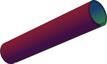
Figure 1. Nanoscroll topology.
Download figure:
Standard image High-resolution image
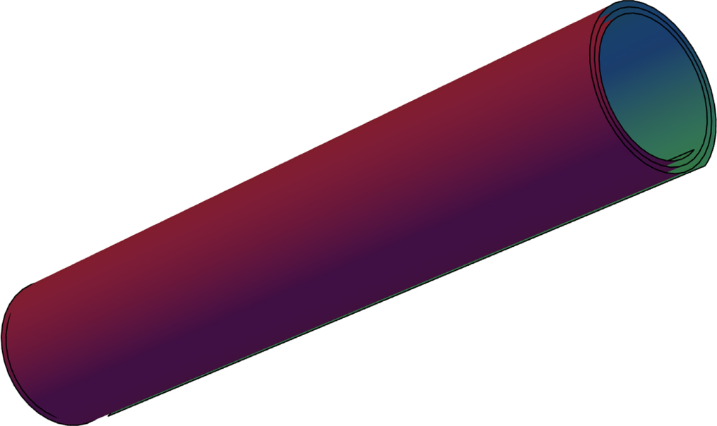
Figure 2. Parametric plot for r(φ)/R, with D = 25 and N = 5.
Download figure:
Standard image High-resolution imageThe functions and can be obtained using equations (54), (60), depending on the number of windings N and parameter D. In figures 3, 4, we plot them for N = 5 and D = 120.


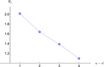
Figure 3. Example of the function for N = 5, D = 120.

Download figure:
Standard image High-resolution image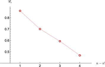
Figure 4. Example of the function for N = 5, D = 120.

Download figure:
Standard image High-resolution imageThe poles of the function come from (63). In particular, if we choose R = 90 nm, N = 5 and D = 120, we find:


We expect unconventional optical responses from the nanoscroll sample in a range of energy [0.4 ÷ 5] eV. Remarkably, the latter energy interval includes the visible light energy range.
In figures 5, 6, 7, 8 we plot the real part of the longitudinal optical conductivity as a function of the energy Ω, for interband and intraband transitions of a nanoscroll geometry with number of windings N = 5. As expected from our analysis, the intraband transitions are in general suppressed, except for narrow peaks around the singular points (66). The interband transitions, on the contrary, show optical responses for the expected energy ranges. The zeros of the interband transitions exactly occur for the points identified by (64). In figure 9 we plot for interband transitions with N = 3. For the latter number of windings, the intraband transition features strongly suppressed values of the optical conductivity ( has isolated peaks with maximum values of the order of 10−10 or less). Finally, in figure 10 we plot for the same parameters but a different chemical potential. 12 We can see that this requires larger minimum energy to observe optical responses: in particular, the critical incident light energy triggering the transition increases as the chemical potential rises [91].
![$\mathrm{Re}[{\sigma }_{\mu \mu }]$](https://content.cld.iop.org/journals/1402-4896/97/6/064005/revision2/psac6d22ieqn61.gif)
![$\mathrm{Re}[{\sigma }_{\varphi \varphi }^{\mathrm{inter}}]$](https://content.cld.iop.org/journals/1402-4896/97/6/064005/revision2/psac6d22ieqn62.gif)
![$\mathrm{Re}[{\sigma }_{\varphi \varphi }^{\mathrm{inter}}]/{{ \mathcal I }}_{S}$](https://content.cld.iop.org/journals/1402-4896/97/6/064005/revision2/psac6d22ieqn63.gif)
![$\mathrm{Re}[{\sigma }_{\varphi \varphi }^{\mathrm{inter}}]$](https://content.cld.iop.org/journals/1402-4896/97/6/064005/revision2/psac6d22ieqn64.gif)

Figure 5. Real part of the interband longitudinal optical conductivity for a nanoscroll geometry with parameters N = 5, D = 120, R = 90 nm, T = 300 K, .
![$\mathrm{Re}[{\sigma }_{\varphi \varphi }^{\mathrm{inter}}]$](https://content.cld.iop.org/journals/1402-4896/97/6/064005/revision2/psac6d22ieqn65.gif)

Download figure:
Standard image High-resolution image
Figure 6. Real part of the intraband longitudinal optical conductivity for a nanoscroll geometry with parameters N = 5, D = 120, R = 90 nm, T = 300 K, .
![$\mathrm{Re}[{\sigma }_{\varphi \varphi }^{\mathrm{intra}}]$](https://content.cld.iop.org/journals/1402-4896/97/6/064005/revision2/psac6d22ieqn67.gif)

Download figure:
Standard image High-resolution image
Figure 7. Real part of the interband longitudinal optical conductivity for a nanoscroll geometry with parameters N = 5, D = 120, R = 90 nm, T = 300 K, .
![$\mathrm{Re}[{\sigma }_{{zz}}^{\mathrm{inter}}]$](https://content.cld.iop.org/journals/1402-4896/97/6/064005/revision2/psac6d22ieqn69.gif)

Download figure:
Standard image High-resolution image
Figure 8. Real part of the intraband longitudinal optical conductivity for a nanoscroll geometry with parameters N = 5, D = 120, R = 90 nm, T = 300 K, .
![$\mathrm{Re}[{\sigma }_{{zz}}^{\mathrm{intra}}]$](https://content.cld.iop.org/journals/1402-4896/97/6/064005/revision2/psac6d22ieqn71.gif)

Download figure:
Standard image High-resolution image
Figure 9. Real part of the interband longitudinal optical conductivity for a nanoscroll geometry with parameters N = 3, D = 120, R = 90 nm, T = 300 K, .
![$\mathrm{Re}[{\sigma }_{\varphi \varphi }^{\mathrm{inter}}]$](https://content.cld.iop.org/journals/1402-4896/97/6/064005/revision2/psac6d22ieqn73.gif)

Download figure:
Standard image High-resolution image
Figure 10. Real part of the interband longitudinal optical conductivity for a nanoscroll geometry with parameters N = 3, D = 120, R = 90 nm, T = 300 K, .
![$\mathrm{Re}[{\sigma }_{\varphi \varphi }^{\mathrm{inter}}]$](https://content.cld.iop.org/journals/1402-4896/97/6/064005/revision2/psac6d22ieqn75.gif)

Download figure:
Standard image High-resolution imageThe massless formulation for charge carriers in graphene nanoscrolls has been recently studied in [87], the gapless nature of the material being preserved especially for high overlap ratio (as it happens for our multiple wrapped surfaces).
5. Concluding remarks
A deeper intertwining of different scientific areas has always proved to be a powerful tool for improving our understanding of many fascinating physical aspects of our world. In particular, by intersecting outcomes from condensed matter and high energy physics, many developments can be found in a multidisciplinary environment, see e.g. [93–121]. Inspired by these approaches, we combined techniques from general relativity, differential geometry and solid state physics to analyse some interesting properties of quantum modes in a concrete, two–dimensional curved background.
The study of graphene–like materials naturally involves a relativistic quantum field formulation, these special materials realizing the physics of Dirac fermions in a real laboratory system. As we have seen, the presence of curvature may give rise to peculiar physical consequences, that can be interpreted as the analogues of (lower–dimensional) gravitational effects, the deformed layer acting as a curved spacetime. In this paper, in particular, we constructed analytical solution to the Dirac equation in a deformed framework representing a cylindrical nanoscroll topology. We then introduced a suitable Kubo formula for a bidimensional background, deriving a compact form for the real part of the optical conductivity. The latter was exploited to obtain some remarkable experimental predictions about the optical response of the nanoscroll in the visible–light energy range at room temperature T = 300 K. Clearly, the same approach finds application also in different spacetime geometries, like for instance the BTZ geometry [122] that, under certain conditions, may be reproduced in suitable graphene configurations with constant negative curvature [123, 124].
The results have been obtained exploiting a bottom–up formulation, the geometry of the graphene–like substrate affecting the propagation of the quantum fields in the material. The dynamics of the charge carriers therefore depends on an effective metric, so that it is possible to exploit some mathematical tools from General Relativity and quantum field theory in curved spacetime. On the other hand, some studies theorize that graphene–like membranes could realize alternative (unconventional) forms of supersymmetry [125–129], the latter becoming in turn a new tool to inspect the properties of quantum fields in Dirac materials. This kind of construction exploits an holographic top–down approach, where the substrate description originates from an higher–dimensional geometrical formulation of a (super)gravity theory [130, 131]. A more detailed comparison between these two kinds of approach will be pursued in a future work.
Acknowledgments
I would like to thank Profs M Trigiante, G A Ummarino, F Laviano and A Carbone that supported these studies with their funds.
Data availability statement
All data that support the findings of this study are included within the article (and any supplementary files).
Footnotes
- 1
For graphene, one has vF ∼ c/300 .
- 2
- 3
In high energy physics, the Dirac equation emerges from the request of spacetime Lorentz invariance and other general considerations related to special relativity and quantum mechanics.
- 4
The σ bands are well separated in energy (more than 10 eV in the center of the FBZ) and are neglected in calculations, since they are too far away from the Fermi level to play a role.
- 5
A tight–binding model describes electrons in the limit of far apart ions, the single–particle eigenstates referring to a charge carrier affected by a single ion; this results in a set of lattice sites with a single–level state, where the electrons can tunnel to their first neighbour atoms only.
- 6
- 7
The vielbein defines a local set of tangent frames of the spacetime manifold and is expressed as , where ya (x0) denote a coordinate frame inertial at the space-time point x0.
- 8
from now on we work in (pseudo)natural units: ℏ = vF = 1
- 9
Here we consider, for completeness, the generic formulation that takes into account also massive fermions; in the following, we will restrict to the study of Dirac materials featuring massless fermionic charge carriers (m → 0 limit).
- 10
Internal disorder of the sample can be simulated, in the calculations, by performing an ensemble averaging over a distribution of the model parameters [90].
- 11
- 12
The chemical potential of doped graphene can be controlled by chemical doping or external gate voltage [92].

