

Abstract
The effects of external magnetic field, hydrostatic pressure, temperature and radius of the quantum dots (QDs) on refractive index changes (RICs) of tuned QDs are studied in detail theoretically. In the framework of effective mass approximation, energy levels and wave functions are derived. Simultaneously, the nonlinear RICs are obtained by compact-density-matrix approach and iterative method. Then, the numerical simulations show that under various constraint factors, the resonant peak position of RICs moves to high energy or low energy, that is, blue shift or red shift, and the peak value of RICs will also alter with the change of parameters.
Export citation and abstract BibTeX RIS
1. Introduction
At present, the rapid development of the information industry has higher and higher requirements for the integration of integrated circuit devices, which urges people to constantly explore ways to break through the size limit of devices [1–3]. With the in-depth study of submicron and deep submicron, low dimensional semiconductor quantum devices have emerged [4–7]. The development of low dimensional semiconductor materials actually promotes the rapid development of quantum research [8–10]. When approaching or reaching the nano size, the low dimensional semiconductor structure will show some new quantum phenomena and effects. These quantum effects can be used to develop optical communication quantum devices with new functions. They are widely favored by people because of their low transmission loss, great broadband, anti-electromagnetic interference, transmission quality number, good confidentiality, and so on [11–14]. Consequently, the development of the semiconductor materials industry has always been one of the focuses of research.
Various quantum structures will produce different nonlinear optical properties for low dimensional semiconductor quantum devices. Therefore, many researchers have done a lot of work to meet the needs of production and life. In 2016, L. Shi et al [15] theoretically studied the electric field and shape effect on the linear and nonlinear optical absorption coefficients (OACs) and RICs of multi-shell ellipsoidal QDs. In 2020, S. Mo et al [16] found that the exciton effect in quantum wells significantly enhanced linear and nonlinear OACs and RICs. In 2020, M. Kria et al [17] studied the linear and nonlinear OACs and RICs of the donor impurity 1s-1p transition in the AlAs/GaAs cylindrical nuclear shell QDs. In 2021, E.B. Al [18] discussed the influence of size modulation and donor position on intersubbands RICs of a donor within a spherical core/shell/shell semiconductor QDs. In 2021, L. Máthé et al [19] investigated the linear together with the third-order nonlinear OACs and RICs under inversely quadratic Hellmann potential. However, in theory, RICs of tuned QDs in the perpendicular magnetic field, hydrostatic pressure and temperature have not been studied, so the effects of the perpendicular magnetic field and hydrostatic pressure in the tuned QDs will be studied theoretically in this paper.
Driven by these previous works, this paper theoretically studies the effect of the parabolic inverse square confinement potential modulated by a modified Gaussian potential on the RICs in two-dimensional single-electron quantum dot systems. In section 2, we solve the Schrödinger equation, then obtain the analytical expressions of the wave function and energy level, and deduce the simple analytical formula of RICs. Section 3 presents a numerical analysis and discussion. The results show that the perpendicular magnetic field, hydrostatic pressure, and temperature have significant effects on the RICs. Section 4 gives a brief summary.
2. Theory
2.1. Theoretical model
We study a model with modified Gaussian and parabolic inverse square constraint potential, and the electron in the model is affected by a magnetic field perpendicular to its plane. This bound potential in the model  [20] consists of a parabolic and inverse square potential functions in the form

where  is the harmonic confinement frequency,
  is the dimensionless parameter,
  [21–23] is an effective mass, for GaAs/Ga0.7Al0.3As materials connected to temperature
  and hydrostatic pressure
  and it can be expressed as follows

where  is the momentum-dependent energy and is equal to 7.51 eV,
  is the mass of free electron,
  is the spin–orbit splitting energy and is equal to 294.2 meV. The energy gap function
  is related to hydrostatic and temperature, analyzed as follows

among, ![${E}_{g}^{{\rm{\Gamma }}}(0,T)=\left[1.519-(5.405\times {10}^{-4}{T}^{2})/(T+204)\right].$](https://content.cld.iop.org/journals/1402-4896/97/6/065803/revision2/psac6a20ieqn11.gif)
The modified Gaussian potential [13] may be expressed as follows

where  and
and  is the depth of limiting potential and the radius of the quantum dot, respectively. While assuming q = 2 and
  ≪ 1, so that the modified Gaussian potential can be expressed as the harmonic oscillator potential

so the total restricted potential is given by

The Hamiltonian of the stationary electron in the system [24] under the effective mass approximation mode, it is

where  denotes the vector potential, it can be written as
  after using the Coulomb gauge, so the aforementioned Hamiltonian can also be expressed as

where  this model adequately expresses two-dimensional quantum dot, whose confinement potential is in its form in accordance with the transverse electrostatic constraints of the electron in the x-y plane.
The Schrödinger equation can be expressed as

where  is the two-dimensional eigenstates for quantum dot and its form can also be expressed as

where  is the magnetic quantum number. Substitute equations (8) and (10) into the equation (9), we can get
where  to a further replacement for the convenience of the calculation, ordered

Equation (11) becomes

among them, 
 which
which  For further solution, order
 and
and  Substituting into equation (13), can get

because the wave function is asymptotic at the origin and at infinity, it can be supposed

substitute equation (15) into equation (14) to obtain

make  and
and  further simplify, equation (16) can be written as

this formal equation is mathematically solved as a confluent hypergeometric function. To make  finite, order
  we can get

where  is the Euler-Gamma function,
  for the associated Laguerre polynomial, hence

combined equations (12) and (19) are be obtained

so the normalized wave function of the quantum dot obtained by the equation (10) is

where 
 =
= 
The energy eigenvalue of quantum dot system is given by

2.2. Nonlinear optical properties
Assuming that the system is excited by an electromagnetic field, which can be expressed as

the evolution of the density matrix operator  follows the Liouville equation [25]

where  is the un-perturbative density matrix operator,
  is the relaxation rate, and
  is the Hamiltonian for no electromagnetic field system. Equation (24) can be calculated using the iterative method


the electrical polarization of quantum dot due to the electromagnetic field  can be expressed as [26]

among  is the vacuum dielectric constant,


 are the linear susceptibility, the second-harmonic coefficients, the third-harmonic coefficients and the third-order polarizability, respectively. The n-order polarization is

where  is the trace,
  express the volume of the system. Expression for the linear and third-order nonlinear RICs of the integrated available system [27–31]

the total change in the refractive index is

where 
 represents the electron density in the system,
  is the refractive index,
  is the permeability,
  is the incident light intensity,
  is the matrix element.
3. Results and discussion
We will systematically analyze the RICs in GaAs/Ga0.7Al0.3As QDs under a perpendicular magnetic field in this section, mainly discussing the effects of the perpendicular magnetic field  hydrostatic pressure
  temperature
  harmonic confinement frequency
  quantum dot radius
  limiting potential depth
  dimensionless parameters
  and incident light intensity
  The following are the reference values of parameters and variables used in the whole calculation process [18, 21, 27, 30–33]:


Table 1 shows the values of asymmetric dipole matrix elements  and energy level intervals
  at various factor values. It is worth noting that the energy level interval
  will directly affect the moving direction of the resonant peak position of RICs, and the alternation of dipole matrix elements
  mainly determines the change of the peak value of RICs. In figure 1, we draw the function curves of linear, nonlinear and total RICs and incident light energy
  under different quantum dot radii
  = 10, 11, 12 nm, respectively. On one hand, it can be seen from the figure that the resonant peak of RICs shifts to the low-energy region with the growth of the radius size of QDs. This is because the enlargement of the radius of QDs will lead to the diminish of the modified Gaussian potential, then reduce the subband energy level interval of the confined electron. On the other hand, the peak value of RICs will continue to raise with the growth of quantum dot radius. That is because the wave function overlap phenomenon becomes more and more obvious with the build-up of
  and then the dipole matrix element
  enlarges with the increase of quantum dot radius. The corresponding change trends can be found in table 1, regardless of the characteristics of formant position and peak size change under different quantum dot radii.
Table 1. Matrix elements and energy level intervals under various parameter values.
| Parameter | Value | ∣M10∣ (×10−8m) | ΔΕ (×10−20J) |
|---|---|---|---|
| R (nm) | 10 | 0.7071 | 1.9738 |
| 11 | 0.7778 | 1.8290 | |
| 12 | 0.8485 | 1.7106 | |
| V0(meV) | 200 | 0.7425 | 1.6253 |
| 300 | 0.7778 | 1.8290 | |
| 400 | 0.8132 | 1.9804 | |
| ξ | 0.5 | 0.7333 | 1.8290 |
| 1.0 | 0.7778 | 1.8290 | |
| 1.5 | 0.8053 | 1.8290 | |
| ω0(THz) | 30 | 0.8096 | 1.6827 |
| 40 | 0.7778 | 1.8290 | |
| 50 | 0.7460 | 1.9936 | |
| B(T) | 0 | 0.8202 | 1.7524 |
| 8 | 0.7778 | 1.8290 | |
| 16 | 0.7354 | 1.9201 | |
| P(kbar) | 0 | 0.8026 | 2.2558 |
| 10 | 0.7778 | 1.8290 | |
| 20 | 0.7531 | 1.5857 | |
| T(K) | 300 | 0.7392 | 1.4732 |
| 400 | 0.7778 | 1.8290 | |
| 500 | 0.8029 | 2.1630 | |
| I(MW cm−2) | 2 | 0.7778 | 1.8290 |
| 3 | 0.7778 | 1.8290 | |
| 4 | 0.7778 | 1.8290 |

Figure 1. RICs as function of photon energy at different radius of the QDs.
Download figure:
Standard image High-resolution imageThe behavior of the linear, third-order nonlinear and total RICs with the incident photon energy at different limiting potential depths are made in figure 2. From the nine curves in the figure, it can be found that the change trend of the three types of curves is similar, that is, the position of the resonance peak of RICs will blueshift for the growth of the limiting potential depth. In addition, the peak value of RICs will raise with the enlargement of the limiting potential depth. The growth of the limit potential depth will enlarge the energy difference between the first excited state and the ground state, so the position of the resonance peaks will move to the high-energy region. At the same time, the dipole matrix element  will also magnify with the increase of
  The change characteristics of this curve can be found in table 1 from the perspective of numerical value.

Figure 2. RICs along with the change of photon energy at different depths of the confinement potential.
Download figure:
Standard image High-resolution imageAs shown in figure 3, we discussed the effect of the dimensionless parameters on the RICs in the tuned QDs. It can be clearly seen from the figure that the resonant peak position of RICs does not move, because when the magnetic quantum number  takes 0, the energy level interval
  is independent of the dimensionless parameter
  Moreover, the peak value of RICs increases gradually with the growth of dimensionless parameter value. The enlargement of
  will improve the probability of electron transition. Therefore, the peak value of RICs will increase with the enlargement of

Figure 3. RICs along with the change of photon energy under different dimensionless parameters.
Download figure:
Standard image High-resolution imageIn figure 4, the effect of harmonic confinement frequency on the RICs in tuned QDs is discussed and the harmonic confinement frequencies are taken:  = 30, 40, 50 THz, respectively. As can be seen from this figure, the RICs resonance peaks move towards the high-energy region with the harmonic confinement frequency increasing. The physical source of this displacement is the quantum confinement effects in these nanostructures, which cause energy level separation, and the stronger the confinement effect, the more pronounced. We know that with
  increasing, the binding potential
  also increases, and then the quantum restricted effect increases, the
  of confined electron enlarges, therefore, the position of the resonance peak of RICs is blue shifted. At the same time, the figure shows that the RICs magnifies with the growth of harmonic confinement frequency, because the dipole transition matrix elements
  raise with increasing of harmonic confinement frequency, which in turn affects the size of the peak RICs.

Figure 4. RICs along with the change of photon energy at different harmonic confinement frequencies.
Download figure:
Standard image High-resolution imageThe variation of the linear, third-order nonlinear and total RICs as function of the incident photon energy for different hydrostatic pressure values are given in figure 5(a) and we plotted functional relationship between effective mass  of electron and hydrostatic pressure
  in figure 5(b). The RICs resonance peaks move to the low-energy region as the hydrostatic pressure
  increases. As can be seen from figure 5(b), hydrostatic pressure will lead to the increase of the effective mass of electron within the value range, which makes the hydrostatic pressure have the effect similar to diminishing the constraint, resulting in the decrease of the constraint strength. The energy level interval
  between the first excited state and the ground state is reduced by growing the value of hydrostatic pressure. Consequently, by growing the hydrostatic pressure, the resonant peak position of RICs is redshifted. More than this, the peak of RICs observed from the variation diagram decreases with the increase of hydrostatic pressure. We have noticed that there are still many studies on hydrostatic pressure. For example, [20] has the same theoretical model as this paper, but this paper adds the factor of adjustable effective quality, which makes the whole system more flexible. More than this, [7] also obtained similar conclusions, however, it is worth noting that the growth rate of RICs in this paper is higher for hydrostatic pressure, which shows that our system is more sensitive to hydrostatic pressure.

Figure 5. (a) RICs along with the change of photon energy under different hydrostatic pressures; (b) Effective mass of electron as function of hydrostatic pressure.
Download figure:
Standard image High-resolution imageFigure 6(a) illustrates the linear  the third-order nonlinear
  and the total RICs
  as a function of the incident photon frequency, with three different values of temperatures
  It can be seen from the figure that the position of the resonance peak of RICs is blue shifted. As can be seen from figure 6(b), the effective mass of the electron
  decreases with the enhancement of temperature. The decrease of
  will lead to a larger energy difference between the ground state and the first excited state, so the position of the formant moves to the high-energy region. We can also clearly observe that the maximum value of RICs enlarges with the growth of temperature as a consequence of the enlargement of temperature will raise the square of dipole matrix elements. Compared with figure 5, the influence of hydrostatic pressure and temperature on the peak value (resonance peak) of RICs is exactly the opposite, and both external factors directly affect the effective mass of electron, so as to regulate the value of RICs. It is similar to the influence of electric field on RICs in [15] and [31], but this paper makes a detailed study on the effective mass, which makes the whole system more flexible. Once the QDs with a certain structure is prepared, the size and internal parameters of the QDs will be determined. Then we can enhance the performance of the quantum device by adjusting the external environmental conditions.

Figure 6. (a) RICs along with the change of photon energy at different temperatures; (b) Effective mass of electron as function of temperature.
Download figure:
Standard image High-resolution imageThe figure shows the variation of RICs as a function of incident photon energy under different vertical magnetic field values as shown in figure 7. We can clearly see that the peaks of linear, third-order nonlinear and total RICs diminish with the increase of magnetic field B, and the resonant peak position of RICs shifts towards the high-energy region. This is because with the growth of magnetic field, the quantum confinement effect weakens and the energy level interval enhances, resulting in blue shift behavior. These behaviors are fully illustrated in table 1.
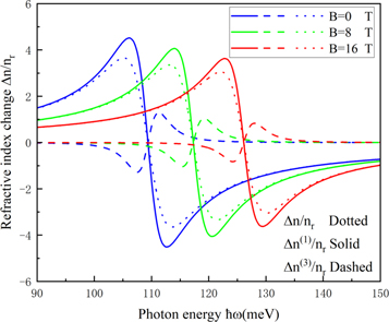
Figure 7. RICs along with the change of photon energy under different vertical magnetic fields.
Download figure:
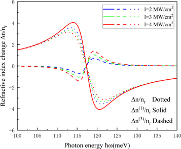
Standard image High-resolution imageAs shown in figure 8, the effect of incident light intensity on the RICs in tuned QDs is discussed and injected light intensities are taken separately:  = 2, 3, 4 MW cm−2. It can be seen from the figure that the peak value of third-order nonlinear RICs raise with the growth of incident light intensity, while the peak value of the total RICs becomes smaller. Because the linear part of RICs is independent of the incident light intensity, and there is no quantitative relationship between the energy level interval
  and
and  the linear RICs under the three incident light intensities overlap into a curve, while the third-order nonlinear RICs has a negative correlation linear relationship with the incident light intensity
  Coincidentally, the data in [34] also show this change.
Figure 8. RICs along with the change of photon energy in situations of several different intensity of incident light.
Download figure:
Standard image High-resolution image
4. Conclusion
Numerical simulations expound that the peaks of RICs will grow with the growth in dimensionless parameter, temperature, quantum dot radius and limiting potential depth, while decrease with the raise of perpendicular magnetic field, hydrostatic pressure and harmonic confinement frequency. Moreover, the enlargement in limiting potential depth, vertical magnetic field, temperature and harmonic confinement frequency can move the RICs resonance peaks towards the high energy direction, however as the hydrostatic pressure and quantum dot radius magnify, the RICs resonance peaks move towards the low energy direction.
Acknowledgments
Project supported by Support National Natural Science Foundation of China (Grant Nos. 52174161, 12174161, 51702003, 61775087, and 11674312), the Natural Science Foundation of Anhui Province (No.1508085QF140) and Plan Fund for Outstanding Young Talents in Colleges and Universities (No. gxyqZD2018039).
Data availability statement
All data that support the findings of this study are included within the article (and any supplementary files).
Ethical statement
I, the Corresponding Author, declare that this manuscript is original, has not been published before and is not currently being considered for publication elsewhere.
Declaration of interest statement
We declare that we have no financial and personal relationships with other people or organizations that can inappropriately influence our work, there is no professional or other personal interest of any nature or kind in any product.