Abstract
In this paper, a novel meshfree approach for three-dimensional free vibration analysis of thick laminated composite conical, cylindrical shells and annular plates is presented. The theoretical model for free vibration analysis of thick shells and plates is formulated by applying the three-dimensional theory of elasticity, and all displacement components are approximated by a novel meshfree Tchebychev-point interpolation method (TPIM) shape function using Tchebychev polynomials as a basis. After deriving the governing equations and boundary conditions for individual layers of the laminated shell, the governing equations and boundary conditions of the entire system are derived by combining them according to the order of layers. The boundary and combination conditions are generalized by introducing the artificial spring technique, and the type of conditions is selected by the spring stiffness values. The accuracy and reliability of the proposed method are verified by comparison with the results of literatures and finite element software ABAQUS. The free vibration characteristics such as the natural frequency and mode shape of laminated conical, cylindrical shells and annular plates under different boundary conditions are presented through some numerical examples.
Export citation and abstract BibTeX RIS
1. Introduction
Thick laminated conical, cylindrical shells and annular plates are very important structures widely used in many engineering fields such as aerospace, shipbuilding and mechanical industry. With the development of science and technology, various composite materials with good performance are used in manufacturing machinery. Among them, fiber-reinforced composite laminates are easy to make and have good performance, so their applications are becoming more and more extensive. By now, there were many studies on static and dynamic characteristic of laminated shell and plate.
In particular, many studies were conducted to more accurately obtain the natural frequency, which is an important technical characteristic of laminated shells and plates. For thin and moderately thick laminated shell and plate, the classical plate theory (CPT), first order shear deformation theory (FSDT) and higher order shear deformation theory (HSDT) were used. CPT is the earliest theory applied in the vibration analysis of composite laminated shell and plate, but it does not consider the transverse shear deformations [1–10]. Therefore, the vibration analysis results of the moderately thick shell and plate using CPT are not very accurate. In order to overcome this defect and to obtain more accurate natural frequencies, FSDT was introduced considering the transverse shear deformations by applying the shear correction factor [11–19]. Qin et al [20] constructed the theoretical models in the framework of FSDT and introduced the multi-segment segmentation strategy to perform free vibration analysis of composite laminated rectangular plates according to arbitrary boundary conditions. Civalek et al [21, 22] conducted studies on free vibration and buckling behavior of carbon nanotube (CNT)-reinforced cross-ply laminated composite and functionally graded plates based on FSDT. In addition, HSDT was applied to consider the transverse shear deformations more correctly in dynamic characteristic analysis of laminated structure [23–26]. However, for more thick shells and plates, it is difficult to obtain accurate natural frequencies through the above theories. In other words, accurate solutions can be determined by applying the three-dimensional theory of elasticity to the free vibration analysis of thick structures.
In the past period, some studies were carried out to calculate the natural frequencies of thick shells and plates using the three-dimensional theory of elasticity. Ye et al [27] developed a unified three-dimensional elasticity method for the free vibration analysis of thick cylindrical shell resting on elastic foundations. In this method, the displacements of shell were expanded as a standard Fourier cosine series. Jin et al [28] conducted three-dimensional free vibration analysis of isotropic and orthotropic conical shells with elastic boundary restraints. Khare et al [29] conducted three-dimensional vibration analysis of the thick laminated circular and annular plates using the finite element method (FEM). Rastogi et al [30] used FEM to conduct three-dimensional free vibration analysis of the isotropic and laminated plates. Gao et al [31] applied a power series expansion method to conduct three-dimensional free vibration analysis of a laminated square plate with piezoelectric layers. Chen et al [32] conducted free vibration analysis of the laminated cylindrical shell using a three-dimensional state-space approach. Malekzadeh [33] used a hybrid method to carry out three-dimensional free vibration analysis of thick laminated annular plates. Tong et al [34] conducted three-dimensional vibration analysis of laminated cylindrical shells using a differential quadrature method. Jin et al [35] took place three-dimensional free vibration analysis of thick functionally graded rectangular plates with general boundary conditions. Ye et al [36] conducted three-dimensional analysis on the free vibration of laminated functionally graded spherical shells with general boundary conditions. Su et al [37] studied three-dimensional vibration of thick functionally graded conical, cylindrical shells and annular plates with arbitrary elastic restraints. Jin et al [38] conducted three-dimensional vibration analysis of thick functionally graded annular sector plates with general boundary conditions. Ye et al [39] conducted three-dimensional vibration analysis of functionally graded sandwich deep open spherical and cylindrical shells with general boundary conditions. As can be seen from the literature review, there are little studies on three-dimensional free vibration analysis of thick laminated shell and plate, and in particular, the free vibration of thick laminated conical shell is rarely mentioned. Unlike functionally graded shells, the material properties of laminated shells change discontinuously with the thickness direction. Therefore, it is difficult to obtain a three-dimensional analysis model of the whole laminated structure.
In this paper, first, the governing equations and boundary conditions of the individual layers of the laminated shell are derived, and then they are combined to obtain those of the whole system. The obtained governing equations and boundary conditions are solved using the meshfree strong form method.
Meshfree method does not have a long history of development, but its idea is very unique and has good computational effect. So, it is increasingly attracting the attention of many scholars, and many studies are being conducted to analyze the static and dynamic characteristics of laminated shells and plates using it [40–48]. As with the other numerical solution methods, the meshfree shape function plays a very important role in ensuring the effectiveness of solution. In addition, the development of more effective shape functions is one of the hottest areas in the research of meshfree methods. The point interpolation method (PIM) is a meshfree interpolation method to construct shape functions using the nodes distributed locally in the developing process of meshfree weak-form methods. PIM is one of series representation methods on functions, and a convenient meshfree shape function possessing Kronecker delta function property can be constructed using it. Up to now, the presented PIM shape functions can be separated into 2 kinds according to the form of basis functions. That is, one is the method using pure polynomial basis functions, and the other is that using radial basis functions. However, when using the traditional PIM shape function to perform vibration analysis of complex laminated structures, it has low accuracy than other methods. Therefore, the development of more effective shape functions is still an important task in the research of meshfree methods.
In this paper, a new TPIM shape function is proposed in which the Tchebychev polynomial basis with exponential convergence behavior is applied to the PIM shape function. The main difference between the proposed TPIM and traditional PIM shape functions is to use Tchebychev polynomial instead of pure polynomial as a basis function. First, three-dimensional free vibration analysis of thick laminated conical shell is conducted by using the proposed method. Then, thick laminated cylindrical shell and annular plate are treated as a special state of thick laminated conical shell. The displacement field in the individual layers of thick laminated conical shell is formulized by the three-dimensional theory of elasticity, and the boundary and combination conditions are generalized by the artificial spring technique. The displacement components in individual layers are approximated using the proposed shape function, and the governing equations and boundary conditions of the individual layers of thick shell are derived using Hamilton's principle. Next, the governing equations and boundary conditions of the entire system are obtained by combining the equations of individual layers through the combination condition that the displacement components of nodes are the same at the interface between layers. In addition, the natural frequencies and mode shapes of thick laminated conical, cylindrical shells and annular plates are obtained by solving the governing equations and boundary conditions of the whole system. The effect of material properties, geometric sizes and lamination schemes on the free vibration of laminated shells and annular plates is proposed with some numerical examples.
2. Theoretical formulations
2.1. Meshfree TPIM(Tchebychev point interpolation method) shape function
The method of using polynomials as basis functions in interpolation is a kind of interpolation technique with a long history and is widely used in various numerical methods. In this paper, a new TPIM shape function using the Tchebychev polynomials as the basis of the meshfree point interpolation shape function is proposed.
At any point x in problem domain, TPIM approximation of field function u( x ) can be defined as follows.

where τj ( x ) is Tchebychev polynomial basis, m is the number of basis, and aj is the unknown coefficients. In the two-dimensional domain, Tchebychev polynomial basis function is as follows.

where Ti (x) is a one-dimensional Tchebychev polynomial.

The above equation can be applied only in the range of x ∈ (−1,1). Therefore, when approximating the two-dimensional field function using Tchebychev polynomials, the problem domain is limited to the range of x, y ∈ (−1,1). In order to obtain the unknown coefficient aj , equation (1) is applied to n nodes in the support domain of x .
The matrix form of equation (4) is

where Us is the vector of nodal function values and a the vector of unknown coefficients.


In equation (5), Tm is as follows.

If n = m, then T m is a square matrix with the dimension of n × n. From equation (5)

Substituting equation (9) into equation (1)

where ΦT ( x ) is the TPIM shape function vector.

From equation (11), the  th derivatives of the shape function are

2.2. Description of the model
Figure 1 shows a thick laminated shell. In here, h is the total thickness of laminated shell. The geometry and coordinate system of the kth layer of laminated shell are shown in figure 2. In the conical shell, α is the cone semi-vertex angle, L the length, and R1 the inner radius of conical shell at the small end. The curvilinear coordinate system (x, θ, y) is introduced to the kth layer of laminated shell, and the displacements in x, θ and y directions are u, v and w. hk is the thickness of kth layer. The distance R between any point of the conical shell and the revolution axis is

Moreover, the cylindrical shell and annular plate are considered as conical shells with α = 0° and α = 90°, respectively.
Figure 1. Configuration of thick laminated shell (a) cross-section of laminated composite shell (b) boundary condition of laminated composite shell.
Download figure:
Standard image High-resolution image
Figure 2. Geometry and coordinate system of one-layered conical, cylindrical shells and annular plate (a) conical shell (b) cylindrical shell (c) annular plate.
Download figure:
Standard image High-resolution image2.3. Governing equation and boundary conditions of laminated thick conical shell
2.3.1. Governing equation and boundary conditions
In the three-dimensional theory of elasticity, displacements of any point are directly represented by three spatial coordinates without considering the rotation components of the middle surface, and the geometrical curvatures of a three-dimensional shell are expressed by the relative displacements of the points. According to the three-dimensional theory of elasticity, the strain-displacement relationship in kth layer of a thick conical shell can be expressed as
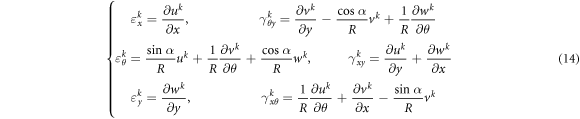
where  and
and  are the normal and shear strain components of kth layer, and uk
, vk
, wk
are the displacement components. In a thick laminated shell, the ply angle of each layer is arbitrary, so the material coordinate system is inconsistent with the curvilinear coordinate system (x, θ, y). Therefore, the constitutive relation of each layer is expressed as follows.
are the normal and shear strain components of kth layer, and uk
, vk
, wk
are the displacement components. In a thick laminated shell, the ply angle of each layer is arbitrary, so the material coordinate system is inconsistent with the curvilinear coordinate system (x, θ, y). Therefore, the constitutive relation of each layer is expressed as follows.

where  and
and  are the normal and shear stress components, and
  is the elastic constants determined by the material parameters and ply angle of kth layer.
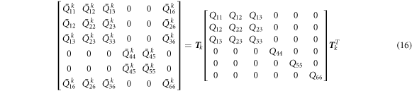
In equation (16), the transformation matrix T k corresponding to the kth layer can be obtained as follows.
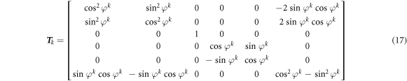
where φk is the ply angle of kth layer.
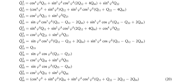
In equation (16), the material elastic stiffness coefficients Qij are as
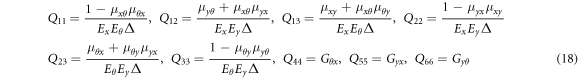
where

From equations (16) and (17),  can be expressed as follows.
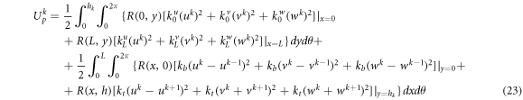
Then, in order to derive the governing equations and boundary conditions in kth layer of thick conical shell, the energy functions have to be obtained. For this, the linear elastic strain energy of shell can be written as the following integral form.

The kinetic energy of kth layer is

where hk is the thickness of kth layer and ρ the density. The potential energy stored in the boundary springs of kth layer is consisted of the energy stored in the boundary of shell with x = 0, L and that stored in the interface between the upper and lower layers.
where 

 are the stiffness values of boundary spring with x = 0, and

 are those of boundary spring with x = L. uk−1, vk−1 and wk−1 are the displacement components on the upper surface of k − 1th layer, and uk+1, vk+1 and wk+1 are those on the lower surface of k + 1th layer. Then, kb
is the combination stiffness value between the lower surface of kth layer and the upper surface of k − 1th layer, and kt
is that between the upper surface of kth layer and the lower surface of k + 1th layer. The combination stiffness values must be large enough to reflect a fixed combination. In the bottom and top layers, kb
= 0 and kt
= 0 , respectively. In the absence of external force, the following equation is established according to Hamilton's principle.
are those of boundary spring with x = L. uk−1, vk−1 and wk−1 are the displacement components on the upper surface of k − 1th layer, and uk+1, vk+1 and wk+1 are those on the lower surface of k + 1th layer. Then, kb
is the combination stiffness value between the lower surface of kth layer and the upper surface of k − 1th layer, and kt
is that between the upper surface of kth layer and the lower surface of k + 1th layer. The combination stiffness values must be large enough to reflect a fixed combination. In the bottom and top layers, kb
= 0 and kt
= 0 , respectively. In the absence of external force, the following equation is established according to Hamilton's principle.

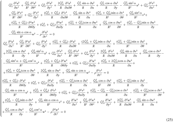
Substituting equations (14), (15), (21)–(23) into equation (24), the governing equation of thick conical shell can be obtained.
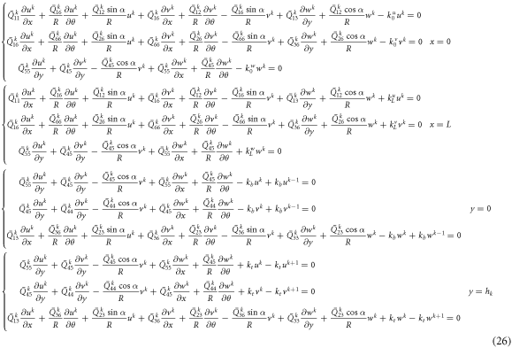
The boundary conditions are
Considering the circumferential symmetry of conical shell, the displacement components of shell can be expanded as a form of modified Fourier series.

After substituting equation (27) into equation (25), multiply the first and third expressions of the governing equation by cos(nθ), and the second expression by sin(nθ). And the expressions are integrated in the range (0, 2π). Considers the following equations.

Then the governing equation can be rewritten as follows.
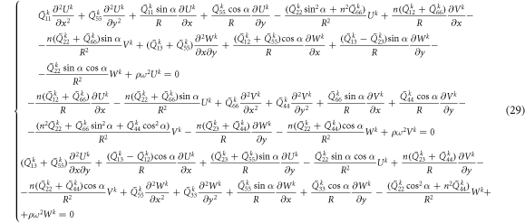
As the same way, the boundary conditions can be rewritten as follows.
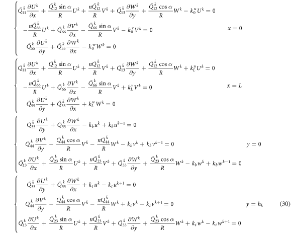
The governing equations and boundary conditions of the cylindrical shell and annular plate can be obtained by taking α = 0° and α = 90° in equations (29) and (30), respectively. The matrix form of the governing equation (29) is as follows.

where the displacement vector u k , mass matrix m k and stiffness matrix k k are expressed as follows.


2.3.2. Meshfree discretization
The problem domain corresponding to the kth layer is discretized into N nodes, and the displacements of a node I in the domain are approximated by the meshfree TPIM shape function Φ( x I ) as

where

where n is the number of nodes in the support domain of node I. In addition, the nodal displacement vector  is as follows.

Substituting equation (35) into equation (31), the nodal discrete equation is obtained.

where the stiffness matrix  and mass matrix
  for node I are expressed as follows.


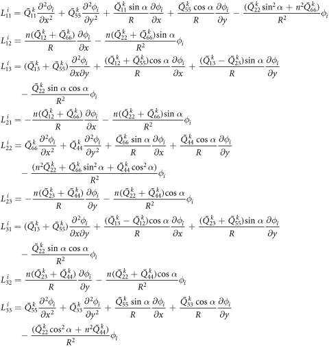
The elements of matrix  are shown in appendix A. In the same way, by establishing nodal discrete equations for all nodes in the problem domain and grouping them according to node number, the discrete equation for the kth layer is obtained.

where the stiffness matrix K k and mass matrix M k for kth layer are


In equation (41),  is the nodal displacement vector for kth layer.

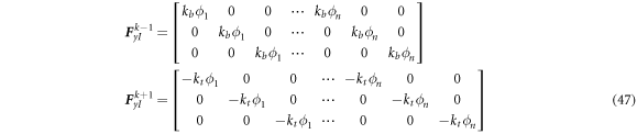
Substituting equation (35) into equation (30), the discretized boundary conditions for kth layer are obtained.

where the coefficient matrices  and
and  are as

The elements of matrixes  and
and  are shown in appendix B. In equation (45),
  and
and  are the coupling matrices between the upper and lower layers.
2.3.3. Combination of governing equation and boundary conditions
The governing equation of the whole system can be obtained by combining the discrete equations of each layers.

where U s is the nodal displacement vector for the whole system. In addition, the stiffness matrix K and mass matrix M for the whole system can be obtained by combining those of each layers.


where Nk
is the number of layers, and 
 are the coupling matrices obtained by arranging the matrices
  and
and  for nodes on the interface according to the number of nodes. The boundary conditions for the whole system can be obtained by combining those of each layers.

3. Numerical results and discussions
3.1. Convergence and verification study
In order to verify the accuracy of the proposed method, the natural frequencies of different laminated shells are obtained using the proposed TPIM shape function and the results are compared with those of literatures and ABAQUS. Table 1 shows the spring stiffness values of foundation corresponding to various boundary conditions used in this paper.
Table 1. Spring stiffness values of different boundaries.
| B.C. | ku | kv | kw |
|---|---|---|---|
| F | 0 | 0 | 0 |
| S1 | 0 | 1015 | 1015 |
| S2 | 1015 | 0 | 1015 |
| S3 | 1015 | 1015 | 0 |
| C | 1015 | 1015 | 1015 |
In tables 2, 3 and 4, the non-dimensional frequencies of thick isotropic conical, cylindrical shells and annular plates obtained by the proposed method are compared with the results of literatures. From the tables, it can be seen that the results obtained by the proposed method agree well with those of the literatures.
Table 2. Comparison of non-dimensional frequencies for isotropic cylindrical shells with different boundary conditions (L/R = 1, h/R = 0.3, μ = 0.3,  ).
).
| m = 1 | m = 2 | m = 3 | |||||
|---|---|---|---|---|---|---|---|
| B. C. | n | [27] | Present | [27] | Present | [27] | Present |
| 1 | 0.0000 | 0.0000 | 0.0001 | 0.0001 | 1.0709 | 1.0707 | |
| 2 | 0.2576 | 0.2577 | 0.3799 | 0.3825 | 1.3532 | 1.3553 | |
| F–F | 3 | 0.6884 | 0.6888 | 0.9252 | 0.9297 | 1.8689 | 1.8711 |
| 4 | 1.2302 | 1.2310 | 1.5158 | 1.5222 | 2.4753 | 2.4773 | |
| 5 | 1.8426 | 1.8440 | 2.1341 | 2.1423 | 3.1169 | 3.1184 | |
| 1 | 0.7516 | 0.7551 | 1.7569 | 1.7560 | 1.8811 | 1.8805 | |
| 2 | 0.6622 | 0.6678 | 1.8982 | 1.8977 | 2.1325 | 2.1307 | |
| C–F | 3 | 0.9247 | 0.9301 | 2.0632 | 2.0636 | 2.5179 | 2.5179 |
| 4 | 1.4021 | 1.4071 | 2.4052 | 2.4067 | 2.9930 | 2.9940 | |
| 5 | 1.9814 | 1.9865 | 2.8687 | 2.8713 | 3.5259 | 3.5272 | |
| 1 | 1.7911 | 1.7900 | 2.6049 | 2.6050 | 3.4259 | 3.4240 | |
| 2 | 1.7507 | 1.7495 | 3.2948 | 3.2950 | 3.5027 | 3.5006 | |
| C–C | 3 | 1.8921 | 1.8909 | 3.6111 | 3.6094 | 3.9443 | 3.9456 |
| 4 | 2.2012 | 2.2002 | 3.8204 | 3.8187 | 4.2781 | 4.2791 | |
| 5 | 2.6421 | 2.6414 | 4.1375 | 4.1358 | 4.7028 | 4.7037 | |
Table 3. Comparison of non-dimensional frequencies for isotropic conical shells with different thickness parameters (R1/L = 0.25, α = 30°, E = 168 GPa, ρ = 5700 kg m−3, μ = 0.3,  ).
).
| F–F | C–C | ||||||||
|---|---|---|---|---|---|---|---|---|---|
| n | Mode | h/L = 0.25 | h/L = 1 | h/L = 0.25 | h/L = 1 | ||||
| [28] | Present | [28] | Present | [28] | Present | [28] | Present | ||
| 0 | 1 | 1.928 | 1.928 | 1.274 | 1.272 | 3.049 | 3.051 | 3.171 | 3.172 |
| 2 | 2.956 | 2.951 | 1.880 | 1.879 | 3.226 | 3.226 | 3.310 | 3.303 | |
| 3 | 3.523 | 3.508 | 3.218 | 3.219 | 4.733 | 4.740 | 4.865 | 4.865 | |
| 4 | 3.650 | 3.656 | 3.650 | 3.652 | 5.740 | 5.748 | 5.351 | 5.354 | |
| 1 | 1 | 2.158 | 2.161 | 1.768 | 1.765 | 2.483 | 2.485 | 3.000 | 2.995 |
| 2 | 2.965 | 2.965 | 1.961 | 1.960 | 4.295 | 4.298 | 3.650 | 3.649 | |
| 3 | 3.476 | 3.481 | 3.622 | 3.621 | 4.839 | 4.845 | 5.203 | 5.211 | |
| 4 | 5.168 | 5.158 | 3.963 | 3.962 | 5.462 | 5.466 | 5.498 | 5.504 | |
| 2 | 1 | 0.618 | 0.620 | 0.786 | 0.786 | 2.555 | 2.558 | 3.203 | 3.196 |
| 2 | 1.468 | 1.464 | 1.076 | 1.074 | 4.900 | 4.904 | 4.248 | 4.249 | |
| 3 | 3.004 | 3.003 | 2.774 | 2.766 | 5.532 | 5.538 | 5.330 | 5.341 | |
| 4 | 3.696 | 3.705 | 2.799 | 2.798 | 6.393 | 6.394 | 5.828 | 5.826 | |
| 3 | 1 | 1.496 | 1.506 | 1.687 | 1.685 | 3.323 | 3.325 | 3.766 | 3.756 |
| 2 | 3.095 | 3.087 | 2.198 | 2.191 | 5.530 | 5.534 | 4.984 | 4.989 | |
| 3 | 4.224 | 4.219 | 3.667 | 3.654 | 6.573 | 6.578 | 5.581 | 5.589 | |
| 4 | 4.791 | 4.811 | 3.732 | 3.732 | 7.932 | 7.935 | 6.244 | 6.240 | |
| 4 | 1 | 2.508 | 2.523 | 2.537 | 2.534 | 4.439 | 4.441 | 4.411 | 4.395 |
| 2 | 4.448 | 4.442 | 3.157 | 3.147 | 6.566 | 6.569 | 5.687 | 5.694 | |
| 3 | 5.438 | 5.431 | 4.404 | 4.397 | 7.755 | 7.758 | 6.100 | 6.113 | |
| 4 | 6.497 | 6.502 | 4.515 | 4.515 | 9.001 | 9.004 | 6.693 | 6.687 | |
Table 4. Comparison of first six non-dimensional frequencies for isotropic annular plates with different boundary conditions (L = 3.5 m, R1 = 1.5 m, h = 1m, E = 206.8428 GPa, μ = 0.29, G = 77.4971 GPa, 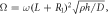 D = Eh3/12(1-μ2)).
| B. C. | Method | Ω1 | Ω2 | Ω3 | Ω4 | Ω5 | Ω6 |
|---|---|---|---|---|---|---|---|
| C-C | 3D FEM ([29]) | 28.888 | 29.474 | 32.256 | 37.797 | 45.810 | 55.339 |
| 3D Ritz ([29]) | 30.743 | 31.474 | 34.370 | 40.266 | 48.736 | 53.072 | |
| Present | 30.621 | 31.333 | 34.184 | 40.029 | 47.745 | 52.711 | |
| S-S | 3D FEM ([29]) | 17.167 | 18.150 | 22.614 | 22.620 | 26.116 | 27.121 |
| 3D Ritz ([29]) | 18.328 | 20.113 | 25.256 | 25.424 | 28.019 | 28.316 | |
| Present | 18.158 | 19.905 | 25.154 | 25.352 | 28.280 | 28.424 | |
| F-F | 3D FEM ([29]) | 4.315 | 7.363 | 10.429 | 14.191 | 14.191 | 17.673 |
| 3D Ritz ([29]) | 4.620 | 7.894 | 11.143 | 15.189 | 15.662 | 18.826 | |
| Present | 4.612 | 7.887 | 11.204 | 15.084 | 15.540 | 18.872 | |
| F-C | 3D FEM ([29]) | 9.772 | 14.994 | 24.027 | 33.980 | 35.126 | 37.800 |
| 3D Ritz ([29]) | 10.448 | 16.026 | 25.650 | 36.220 | 37.346 | 39.602 | |
| Present | 10.514 | 15.998 | 25.519 | 36.029 | 37.164 | 39.481 | |
| F-S | 3D FEM ([29]) | 4.236 | 10.426 | 14.638 | 14.639 | 19.270 | 26.031 |
| 3D Ritz ([29]) | 4.540 | 11.240 | 15.742 | 15.904 | 20.852 | 27.931 | |
| Present | 4.565 | 11.139 | 15.786 | 15.859 | 20.695 | 27.989 |
In table 5, the natural frequencies of orthotropic conical shells with various cone semi-vertex angles and thicknesses obtained by TPIM shape function are compared with those of literatures. The material properties are E1 = 137.9 GPa, E2 = E3 = 8.963 GPa, μ12 = μ13 = 0.3, μ23 = 0.49, G12 = G13 = 7.101 GPa, G23 = 6.205 GPa and ρ = 1605 kg m−3 . In table 6, the natural frequencies of thick laminated conical shells with various cone semi-vertex angles obtained by the proposed method are compared with the results of finite element software ABAQUS. The material properties of laminated shell are E1 = 150 GPa, E2 = E3 = 10 GPa, μ12 = μ13 = μ23 = 0.25, G12 = G13 = 6 GPa, G23 = 5 GPa and ρ = 1450 kg m−3 . In the ABAQUS, the element type is C3D8R, and the number of element is 14800. From tables 5 and 6, it can be seen that the natural frequencies of orthotropic laminated shell obtained by the proposed method agree well with those of literature and ABAQUS. In figures 3, 4 and 5, the four mode shapes of laminated conical shell with cone semi-vertex angle of α = 30°, cylindrical shell and annular plate are compared with the results of ABAQUS.
Table 5. Comparison of natural frequencies of thick orthotropic conical shells with various cone semi-vertex angles and thicknesses (Lcos α = 2 m, R1 = 1 m).
| C-C | S2-S2 | C-S2 | |||||
|---|---|---|---|---|---|---|---|
| α | h/R1 | [27] | Present | [27] | Present | [27] | Present |
| 15° | 0.1 | 253.10 | 253.14 | 170.45 | 169.69 | 194.49 | 194.50 |
| 0.2 | 362.08 | 362.17 | 210.05 | 209.41 | 196.62 | 196.64 | |
| 0.5 | 460.17 | 459.98 | 218.22 | 218.00 | 202.55 | 202.56 | |
| 1.0 | 489.29 | 488.13 | 197.06 | 196.86 | 210.67 | 210.69 | |
| 30° | 0.1 | 203.91 | 203.93 | 138.93 | 138.33 | 137.69 | 137.70 |
| 0.2 | 302.26 | 302.35 | 173.31 | 172.80 | 139.97 | 139.97 | |
| 0.5 | 401.82 | 401.72 | 182.48 | 182.33 | 146.47 | 146.47 | |
| 1.0 | 434.25 | 433.36 | 170.57 | 170.43 | 156.00 | 156.02 | |
| 45° | 0.1 | 139.11 | 139.11 | 102.35 | 101.90 | 87.39 | 87.35 |
| 0.2 | 215.35 | 215.43 | 133.76 | 133.37 | 88.97 | 88.94 | |
| 0.5 | 311.01 | 311.02 | 145.61 | 145.50 | 93.60 | 93.57 | |
| 1.0 | 345.90 | 345.43 | 141.11 | 141.04 | 100.79 | 100.77 | |
| 60° | 0.1 | 72.28 | 72.28 | 60.27 | 60.05 | 44.60 | 44.20 |
| 0.2 | 116.99 | 117.03 | 88.10 | 87.91 | 45.32 | 44.95 | |
| 0.5 | 193.11 | 193.20 | 104.78 | 104.69 | 47.45 | 47.16 | |
| 1.0 | 230.06 | 229.98 | 104.94 | 104.98 | 50.91 | 50.70 | |
Table 6. Comparison of natural frequencies of thick laminated conical shells with various cone semi-vertex angles and boundary conditions (L = 2m, R1 = 1m, h = 0.4m, [0°/90°]).
| Natural frequencies(Hz) | ||||||||||
|---|---|---|---|---|---|---|---|---|---|---|
| α | B.C. | Method | 1 | 2 | 3 | 4 | 5 | 6 | 7 | 8 |
| 0° | C-C | ABAQUS | 389.22 | 389.22 | 412.92 | 412.92 | 485.87 | 485.87 | 508.13 | 663.32 |
| Present | 391.28 | 391.28 | 413.99 | 413.99 | 489.31 | 489.31 | 508.54 | 667.73 | ||
| C-F | ABAQUS | 179.81 | 179.81 | 186.82 | 186.82 | 254.11 | 352.85 | 352.85 | 445.49 | |
| Present | 181.22 | 181.22 | 189.25 | 189.25 | 254.27 | 355.84 | 355.84 | 447.53 | ||
| 5° | C-C | ABAQUS | 384.76 | 384.76 | 413.09 | 413.09 | 463.35 | 463.35 | 508.52 | 617.87 |
| Present | 386.70 | 386.70 | 414.14 | 414.14 | 466.60 | 466.60 | 508.90 | 622.08 | ||
| C-F | ABAQUS | 162.94 | 162.94 | 165.61 | 165.61 | 233.91 | 300.06 | 300.06 | 434.17 | |
| Present | 164.70 | 164.70 | 166.27 | 166.27 | 234.04 | 303.27 | 303.27 | 435.95 | ||
| F-C | ABAQUS | 192.49 | 192.49 | 196.13 | 196.13 | 275.14 | 342.32 | 342.32 | 450.53 | |
| Present | 194.20 | 194.20 | 197.26 | 197.26 | 275.29 | 345.04 | 345.04 | 452.37 | ||
| 15° | C-C | ABAQUS | 379.11 | 379.11 | 412.09 | 412.09 | 433.61 | 433.61 | 510.70 | 553.45 |
| Present | 380.62 | 380.62 | 412.99 | 412.99 | 436.26 | 436.26 | 511.02 | 557.07 | ||
| C-F | ABAQUS | 130.41 | 130.41 | 142.55 | 142.55 | 202.26 | 227.51 | 227.51 | 373.01 | |
| Present | 131.68 | 131.68 | 143.71 | 143.71 | 202.35 | 230.01 | 230.01 | 375.94 | ||
| F-C | ABAQUS | 205.45 | 205.45 | 222.99 | 222.99 | 311.48 | 327.81 | 327.81 | 460.75 | |
| Present | 206.59 | 206.59 | 223.61 | 223.61 | 311.62 | 329.86 | 329.86 | 461.71 | ||
| 30° | C-C | ABAQUS | 372.53 | 372.53 | 405.01 | 405.01 | 409.37 | 409.37 | 498.19 | 498.19 |
| Present | 373.61 | 373.61 | 405.80 | 405.80 | 411.38 | 411.38 | 501.30 | 501.30 | ||
| C-F | ABAQUS | 101.90 | 101.90 | 116.39 | 116.39 | 166.76 | 166.76 | 169.35 | 272.30 | |
| Present | 102.61 | 102.61 | 117.29 | 117.29 | 168.40 | 168.40 | 170.39 | 275.33 | ||
| F-C | ABAQUS | 222.48 | 222.48 | 247.54 | 247.54 | 318.40 | 318.40 | 354.27 | 457.40 | |
| Present | 222.59 | 222.59 | 247.63 | 247.63 | 319.55 | 319.55 | 354.39 | 459.7 | ||
| 90° | C-C | ABAQUS | 332.32 | 332.32 | 334.08 | 344.56 | 344.56 | 387.48 | 387.48 | 460.07 |
| Present | 334.20 | 334.20 | 335.87 | 346.85 | 346.85 | 390.50 | 390.50 | 463.82 | ||
| C-F | ABAQUS | 62.55 | 62.55 | 69.12 | 69.12 | 87.33 | 113.96 | 113.96 | 117.35 | |
| Present | 63.17 | 63.17 | 70.73 | 70.73 | 89.42 | 115.28 | 115.28 | 118.70 | ||
| F-C | ABAQUS | 141.44 | 157.20 | 157.20 | 232.70 | 232.70 | 331.33 | 331.33 | 427.04 | |
| Present | 142.77 | 157.70 | 157.70 | 233.79 | 233.79 | 334.06 | 334.06 | 427.60 | ||
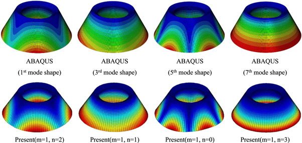
Figure 3. Mode shape comparison of laminated conical shell (C-F, α = 30°).
Download figure:
Standard image High-resolution image
Figure 4. Mode shape comparison of laminated cylindrical shell (C–C).
Download figure:
Standard image High-resolution image
Figure 5. Mode shape comparison of annular plate (F–C).
Download figure:
Standard image High-resolution imageThen, the convergence study on boundary spring stiffness is conducted. In this study, the geometric sizes of laminated shells and annular plate are L = 2 m, R1 = 1 m, h = 0.4 m, and material properties are E1 = 125 GPa, E2 = E3 = 10GPa, μ12 = 0.4, μ13 = μ23 = 0.2, G12 = G23 = 5.9 GPa, G13 = 3 GPa and ρ = 1643 kg m−3. The fiber direction is [0°/90°] and cone semi-vertex angle is α = 30°. In order to investigate the convergence of boundary spring stiffness, one boundary of the laminated shell is set as an elastic boundary and the other boundaries are fixed. Figure 6 shows the change of non-dimensional frequencies  according to the spring stiffness values of elastic boundary in laminated conical, cylindrical shells and annular plate. As shown in figure 6, the non-dimensional frequencies are rapidly changed in the spring stiffness value range of 108–1013, and then they are maintained in a stable value. Therefore, the spring stiffness value of clamped boundary can be set to 1015 as table 1.

Figure 6. Convergence of non-dimensional frequencies on the boundary spring stiffness (a) Conical shell (b) Cylindrical shell (c) Annular plate.
Download figure:
Standard image High-resolution image3.2. Numerical example
In this subsection, the study on vibration characteristics of laminated conical, cylindrical shells and annular plates with various boundary conditions, lamination structures, material properties and geometric sizes is conducted. First, the effect of fiber direction of thick laminated shell on the change of non-dimensional natural frequency is considered. Figure 7 shows the change of non-dimensional frequency  according to the ply angle φ of middle layer in the three-layered [0°/φ/0°] conical, cylindrical shells and annular plates with C–C and S1-S1 boundary conditions. The geometric sizes and material properties are the same as figure 6. As can be seen in figure 7, the five non-dimensional frequencies are symmetric about the axis φ = 90°, smallest at φ = 0° and largest around φ = 60° or φ = 90°.
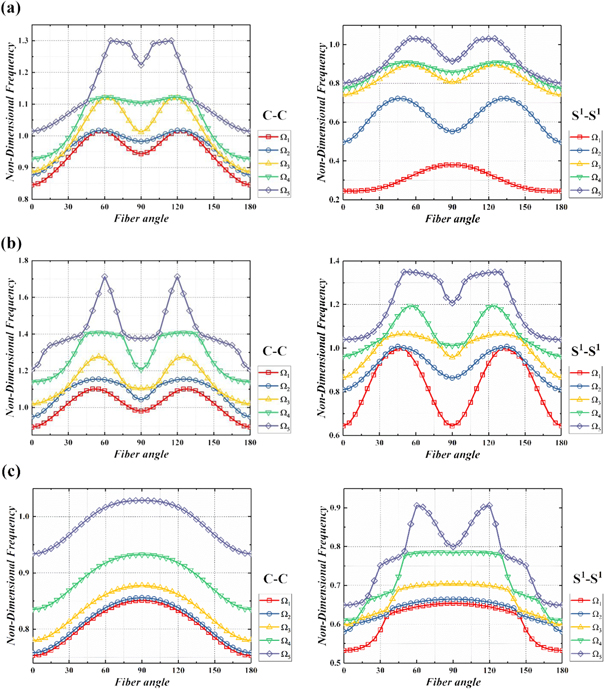
Figure 7. Change in non-dimensional frequencies according to fiber direction of middle layer (a) Conical shell (b) Cylindrical shell (c) Annular plate.
Download figure:
Standard image High-resolution imageThen, the change of non-dimensional frequencies according to Young's modulus ratio is considered. Figure 8 shows the change of Ω according to Young's modulus ratio E1/E2 in the laminated conical, cylindrical shells and annular plate with the thickness of h = 0.3m and the fiber direction of [0°/45°/0°]. The cone semi-vertex angle of laminated conical shell is α = 15°, and other geometric sizes and material properties are the same as figure 6.
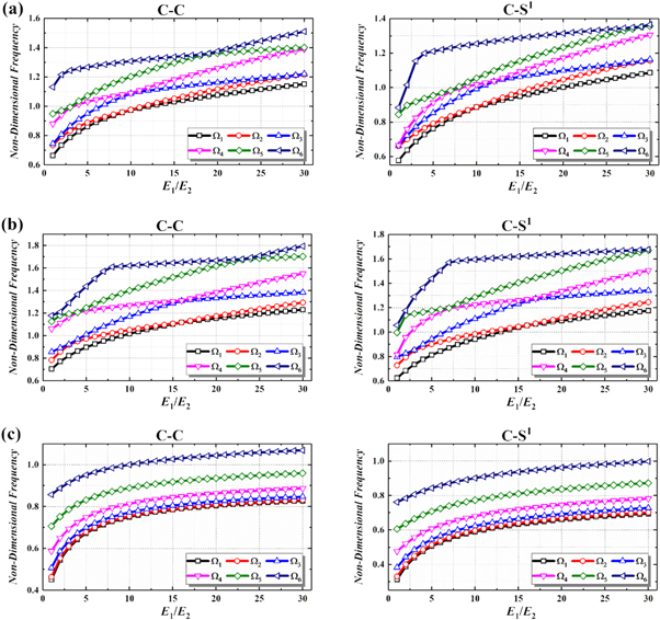
Figure 8. Change in non-dimensional frequencies according to Young's modulus ratio (a) Conical shell (b) Cylindrical shell (c) Annular plate.
Download figure:
Standard image High-resolution imageFrom figure 8, it can be seen that the non-dimensional frequency increases with the increase of the Young's modulus ratio regardless of the boundary conditions.
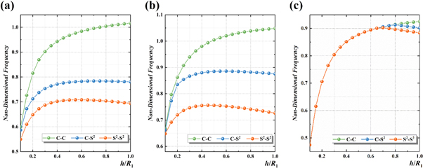
Then, the change of fundamental frequencies according to the thickness of laminated shell is considered. Figure 9 shows the change of non-dimensional fundamental frequencies according to the thickness ratio in the laminated conical, cylindrical shells and annular plate with fiber direction of [0°/90°/0°]. The cone semi-vertex angle of laminated conical shell is α = 30°, and other geometric sizes and material properties are the same as figure 6. In this study, the three types of boundary conditions are considered. From figure 9, it can be seen that the non-dimensional fundamental frequency increases with the increase of the thickness ratio under the C–C boundary condition. When the thickness ratio passes certain limit, the fundamental frequency decreases gradually under C-S2 and S2-S2 boundary conditions. In the conical and cylindrical shells, the non-dimensional fundamental frequencies under the three boundary conditions have a clear difference regardless of the thickness ratio. However, in the annular plate, the non-dimensional fundamental frequencies under the three boundary conditions are similar in the region of thickness ratio of 0–0.6. In other words, it can be seen that the fundamental frequency of the annular plate with a thickness ratio less than a certain value is not significantly related to the circumferential degree of freedom of nodes on the boundaries.
Figure 9. Change in non-dimensional fundamental frequencies according to thickness parameter (a) Conical shell (b) Cylindrical shell (c) Annular plate.
Download figure:
Standard image High-resolution image
Tables 7–9 show the non-dimensional frequencies of laminated conical, cylindrical shells and annular plates according to the length parameter under various boundary conditions. As can be seen from tables, as L/R1 increases, the non-dimensional frequencies decrease for all boundary conditions. This is because when length parameter increases, the stiffness of the structure decreases. Table 10 shows the non-dimensional frequencies of thick laminated conical shells with various cone semi-vertex angles and boundary conditions. It is obvious that the non-dimensional frequencies of the conical shell can be decreased by increasing the cone semi-vertex angle. Tables 11–13 show the non-dimensional frequencies of laminated conical, cylindrical shells and annular plate with different lamination structures and boundary conditions. As shown in tables 11–13, there is no clear regulation in the change of non-dimensional frequencies, but the fundamental frequencies of conical and cylindrical shells are the smallest in two-layered structures and the largest in five-layered structures. In tables 7–13, the material properties are the same as table 5.
Table 7. Non-dimensional frequencies of laminated conical shells with various length parameters and boundary conditions (R1 = 1m, h = 0.3m, [0°/45°/0°], α = 30°).
| Boundary condition | ||||||||||
|---|---|---|---|---|---|---|---|---|---|---|
| L/R1 | Ω | C-C | C-S1 | C-S2 | C-S3 | S1-S1 | S2-S2 | S3-S3 | C-F | F-C |
| 1 | 1 | 2.608 | 2.320 | 1.683 | 1.334 | 0.495 | 1.027 | 0.966 | 0.952 | 1.259 |
| 2 | 2.616 | 2.323 | 1.907 | 1.341 | 1.089 | 1.936 | 0.969 | 0.959 | 1.300 | |
| 3 | 2.626 | 2.335 | 2.308 | 1.374 | 1.982 | 2.390 | 1.002 | 1.037 | 1.322 | |
| 4 | 2.638 | 2.372 | 2.489 | 1.458 | 2.200 | 2.551 | 1.112 | 1.066 | 1.380 | |
| 2 | 1 | 1.210 | 1.036 | 0.700 | 0.733 | 0.327 | 0.697 | 0.675 | 0.347 | 0.654 |
| 2 | 1.216 | 1.041 | 0.911 | 0.755 | 0.819 | 1.026 | 0.689 | 0.359 | 0.688 | |
| 3 | 1.278 | 1.088 | 1.082 | 0.763 | 0.944 | 1.131 | 0.734 | 0.441 | 0.811 | |
| 4 | 1.281 | 1.107 | 1.154 | 0.788 | 0.948 | 1.239 | 0.773 | 0.467 | 0.894 | |
| 3 | 1 | 0.738 | 0.611 | 0.400 | 0.510 | 0.223 | 0.475 | 0.484 | 0.178 | 0.445 |
| 2 | 0.750 | 0.633 | 0.565 | 0.516 | 0.561 | 0.632 | 0.495 | 0.199 | 0.483 | |
| 3 | 0.803 | 0.683 | 0.658 | 0.570 | 0.582 | 0.694 | 0.557 | 0.262 | 0.626 | |
| 4 | 0.836 | 0.718 | 0.704 | 0.573 | 0.621 | 0.785 | 0.567 | 0.284 | 0.669 | |
| 4 | 1 | 0.510 | 0.416 | 0.263 | 0.383 | 0.173 | 0.348 | 0.367 | 0.103 | 0.291 |
| 2 | 0.527 | 0.444 | 0.398 | 0.401 | 0.386 | 0.441 | 0.388 | 0.132 | 0.387 | |
| 3 | 0.568 | 0.476 | 0.456 | 0.425 | 0.415 | 0.482 | 0.417 | 0.165 | 0.510 | |
| 4 | 0.621 | 0.546 | 0.487 | 0.464 | 0.459 | 0.557 | 0.462 | 0.210 | 0.520 | |
| 5 | 1 | 0.381 | 0.308 | 0.187 | 0.305 | 0.146 | 0.273 | 0.294 | 0.151 | 0.290 |
| 2 | 0.401 | 0.339 | 0.304 | 0.329 | 0.290 | 0.335 | 0.318 | 0.187 | 0.311 | |
| 3 | 0.429 | 0.357 | 0.343 | 0.334 | 0.321 | 0.361 | 0.329 | 0.285 | 0.410 | |
| 4 | 0.496 | 0.446 | 0.363 | 0.393 | 0.349 | 0.421 | 0.391 | 0.298 | 0.411 | |
Table 8. Non-dimensional frequencies of laminated cylindrical shells with various length parameters and boundary conditions (R1 = 1m, h = 0.3m, [0°/45°/0°]).
| Boundary condition | |||||||||
|---|---|---|---|---|---|---|---|---|---|
| L/R1 | Ω | C-C | C-S1 | C-S2 | C-S3 | S1-S1 | S2-S2 | S3-S3 | C-F |
| 1 | 1 | 2.697 | 2.489 | 2.121 | 1.685 | 1.184 | 1.179 | 1.289 | 1.176 |
| 2 | 2.697 | 2.512 | 2.294 | 1.694 | 2.331 | 2.091 | 1.312 | 1.207 | |
| 3 | 2.754 | 2.514 | 2.478 | 1.694 | 2.344 | 2.452 | 1.340 | 1.327 | |
| 4 | 2.789 | 2.531 | 2.577 | 1.789 | 2.357 | 2.792 | 1.379 | 1.428 | |
| 2 | 1 | 1.314 | 1.188 | 1.063 | 1.059 | 1.079 | 0.808 | 0.935 | 0.534 |
| 2 | 1.335 | 1.216 | 1.149 | 1.102 | 1.110 | 1.106 | 0.973 | 0.666 | |
| 3 | 1.470 | 1.362 | 1.201 | 1.211 | 1.184 | 1.262 | 1.129 | 0.712 | |
| 4 | 1.534 | 1.445 | 1.296 | 1.348 | 1.264 | 1.504 | 1.242 | 1.024 | |
| 3 | 1 | 0.841 | 0.748 | 0.709 | 0.757 | 0.671 | 0.583 | 0.697 | 0.336 |
| 2 | 0.913 | 0.835 | 0.769 | 0.831 | 0.766 | 0.737 | 0.775 | 0.464 | |
| 3 | 1.008 | 0.950 | 0.784 | 0.947 | 0.907 | 0.888 | 0.907 | 0.552 | |
| 4 | 1.197 | 1.150 | 0.900 | 1.135 | 1.108 | 1.189 | 1.092 | 0.709 | |
| 4 | 1 | 0.610 | 0.537 | 0.532 | 0.574 | 0.473 | 0.468 | 0.542 | 0.253 |
| 2 | 0.732 | 0.682 | 0.581 | 0.697 | 0.639 | 0.557 | 0.669 | 0.310 | |
| 3 | 0.760 | 0.712 | 0.588 | 0.739 | 0.684 | 0.723 | 0.720 | 0.510 | |
| 4 | 1.063 | 1.044 | 0.727 | 1.044 | 1.023 | 1.042 | 0.964 | 0.532 | |
| 5 | 1 | 0.477 | 0.418 | 0.426 | 0.458 | 0.364 | 0.398 | 0.440 | 0.081 |
| 2 | 0.605 | 0.560 | 0.462 | 0.595 | 0.532 | 0.450 | 0.584 | 0.310 | |
| 3 | 0.642 | 0.610 | 0.480 | 0.625 | 0.583 | 0.639 | 0.610 | 0.426 | |
| 4 | 0.851 | 0.851 | 0.640 | 0.851 | 0.834 | 0.828 | 0.804 | 0.612 | |
Table 9. Non-dimensional frequencies of laminated annular plates with various length parameters and boundary conditions (R1 = 1m, h = 0.3m, [0°/45°/0°]).
| Boundary condition | ||||||||||
|---|---|---|---|---|---|---|---|---|---|---|
| L/R1 | Ω | C-C | C-S1 | C-S2 | C-S3 | S1-S1 | S2-S2 | S3-S3 | C-F | F-C |
| 1 | 1 | 2.449 | 2.095 | 1.341 | 0.939 | 1.004 | 0.974 | 0.250 | 0.747 | 1.039 |
| 2 | 2.454 | 2.107 | 1.608 | 0.962 | 1.314 | 1.928 | 0.506 | 0.748 | 1.070 | |
| 3 | 2.472 | 2.144 | 2.217 | 1.032 | 1.950 | 2.449 | 0.773 | 0.759 | 1.166 | |
| 4 | 2.513 | 2.214 | 2.449 | 1.151 | 1.977 | 2.451 | 1.057 | 0.799 | 1.337 | |
| 2 | 1 | 1.042 | 0.798 | 0.493 | 0.322 | 0.675 | 0.681 | 0.134 | 0.215 | 0.361 |
| 2 | 1.046 | 0.805 | 0.805 | 0.338 | 0.686 | 1.042 | 0.263 | 0.215 | 0.401 | |
| 3 | 1.061 | 0.829 | 1.042 | 0.385 | 0.722 | 1.045 | 0.392 | 0.220 | 0.514 | |
| 4 | 1.098 | 0.880 | 1.046 | 0.462 | 0.791 | 1.059 | 0.531 | 0.247 | 0.685 | |
| 3 | 1 | 0.579 | 0.412 | 0.259 | 0.158 | 0.329 | 0.518 | 0.083 | 0.098 | 0.179 |
| 2 | 0.583 | 0.417 | 0.557 | 0.170 | 0.337 | 0.579 | 0.156 | 0.099 | 0.213 | |
| 3 | 0.595 | 0.434 | 0.579 | 0.203 | 0.364 | 0.582 | 0.230 | 0.101 | 0.317 | |
| 4 | 0.625 | 0.471 | 0.583 | 0.255 | 0.417 | 0.594 | 0.313 | 0.119 | 0.446 | |
| 4 | 1 | 0.364 | 0.247 | 0.159 | 0.094 | 0.193 | 0.364 | 0.054 | 0.051 | 0.050 |
| 2 | 0.367 | 0.250 | 0.364 | 0.102 | 0.198 | 0.366 | 0.100 | 0.058 | 0.154 | |
| 3 | 0.377 | 0.263 | 0.367 | 0.127 | 0.219 | 0.376 | 0.149 | 0.061 | 0.210 | |
| 4 | 0.402 | 0.291 | 0.377 | 0.164 | 0.260 | 0.401 | 0.205 | 0.064 | 0.311 | |
| 5 | 1 | 0.247 | 0.163 | 0.106 | 0.062 | 0.126 | 0.247 | 0.037 | 0.009 | 0.028 |
| 2 | 0.249 | 0.165 | 0.247 | 0.069 | 0.130 | 0.249 | 0.069 | 0.058 | 0.093 | |
| 3 | 0.258 | 0.175 | 0.249 | 0.088 | 0.146 | 0.258 | 0.104 | 0.059 | 0.158 | |
| 4 | 0.278 | 0.197 | 0.258 | 0.115 | 0.178 | 0.278 | 0.138 | 0.060 | 0.228 | |
Table 10. Non-dimensional frequencies of thick laminated conical shells with various cone semi-vertex angles and boundary conditions (R1 = 1m, L = 2.5m, h = 0.3m, [0°/45°/0°]).
| Boundary condition | ||||||||||
|---|---|---|---|---|---|---|---|---|---|---|
| α | Ω | C-C | C-S1 | C-S2 | C-S3 | S1-S1 | S2-S2 | S3-S3 | C-F | F-C |
| 0° | 1 | 1.030 | 0.923 | 0.851 | 0.889 | 0.834 | 0.676 | 0.803 | 0.411 | 0.411 |
| 2 | 1.076 | 0.979 | 0.919 | 0.942 | 0.893 | 0.884 | 0.858 | 0.566 | 0.566 | |
| 3 | 1.197 | 1.123 | 0.949 | 1.075 | 1.060 | 1.033 | 1.017 | 0.592 | 0.592 | |
| 4 | 1.322 | 1.256 | 1.053 | 1.217 | 1.184 | 1.306 | 1.152 | 0.851 | 0.851 | |
| 15° | 1 | 0.981 | 0.849 | 0.638 | 0.746 | 0.153 | 0.612 | 0.693 | 0.307 | 0.496 |
| 2 | 0.987 | 0.862 | 0.788 | 0.746 | 0.778 | 0.826 | 0.698 | 0.349 | 0.569 | |
| 3 | 1.094 | 0.980 | 0.877 | 0.849 | 0.789 | 0.922 | 0.835 | 0.424 | 0.693 | |
| 4 | 1.113 | 1.001 | 0.941 | 0.870 | 0.885 | 1.070 | 0.836 | 0.526 | 0.838 | |
| 30° | 1 | 0.926 | 0.777 | 0.517 | 0.604 | 0.265 | 0.571 | 0.570 | 0.245 | 0.533 |
| 2 | 0.935 | 0.793 | 0.704 | 0.609 | 0.706 | 0.790 | 0.572 | 0.256 | 0.568 | |
| 3 | 0.993 | 0.854 | 0.826 | 0.650 | 0.710 | 0.868 | 0.641 | 0.329 | 0.705 | |
| 4 | 1.013 | 0.861 | 0.883 | 0.683 | 0.722 | 0.967 | 0.661 | 0.354 | 0.766 | |
| 45° | 1 | 0.879 | 0.718 | 0.441 | 0.478 | 0.349 | 0.552 | 0.447 | 0.200 | 0.517 |
| 2 | 0.881 | 0.720 | 0.655 | 0.491 | 0.593 | 0.772 | 0.465 | 0.212 | 0.562 | |
| 3 | 0.917 | 0.741 | 0.795 | 0.499 | 0.643 | 0.837 | 0.477 | 0.259 | 0.626 | |
| 4 | 0.935 | 0.748 | 0.847 | 0.504 | 0.653 | 0.914 | 0.498 | 0.278 | 0.730 | |
| 60° | 1 | 0.828 | 0.647 | 0.393 | 0.364 | 0.409 | 0.553 | 0.332 | 0.173 | 0.468 |
| 2 | 0.838 | 0.648 | 0.637 | 0.366 | 0.522 | 0.768 | 0.333 | 0.189 | 0.495 | |
| 3 | 0.844 | 0.650 | 0.781 | 0.374 | 0.569 | 0.820 | 0.340 | 0.201 | 0.538 | |
| 4 | 0.848 | 0.672 | 0.825 | 0.412 | 0.603 | 0.848 | 0.377 | 0.236 | 0.549 | |
| 75° | 1 | 0.785 | 0.584 | 0.363 | 0.263 | 0.446 | 0.571 | 0.180 | 0.155 | 0.350 |
| 2 | 0.785 | 0.588 | 0.642 | 0.271 | 0.481 | 0.774 | 0.194 | 0.16 | 0.355 | |
| 3 | 0.792 | 0.603 | 0.778 | 0.300 | 0.517 | 0.785 | 0.240 | 0.172 | 0.414 | |
| 4 | 0.820 | 0.639 | 0.785 | 0.354 | 0.569 | 0.803 | 0.316 | 0.186 | 0.540 | |
| 90° | 1 | 0.762 | 0.560 | 0.348 | 0.219 | 0.458 | 0.589 | 0.105 | 0.136 | 0.250 |
| 2 | 0.765 | 0.566 | 0.656 | 0.233 | 0.467 | 0.762 | 0.200 | 0.139 | 0.288 | |
| 3 | 0.779 | 0.586 | 0.762 | 0.272 | 0.498 | 0.765 | 0.296 | 0.141 | 0.394 | |
| 4 | 0.812 | 0.629 | 0.765 | 0.335 | 0.559 | 0.778 | 0.401 | 0.163 | 0.545 | |
Table 11. Non-dimensional frequencies of thick laminated conical shells with different lamination structures and boundary conditions (R1 = 1m, L = 2.5m, h = 0.5m, α = 30°).
| Boundary condition | ||||||||||
|---|---|---|---|---|---|---|---|---|---|---|
| Lamination | Ω | C-C | C-S1 | C-S2 | C-S3 | S1-S1 | S2-S2 | S3-S3 | C-F | F-C |
| 0/90 | 1 | 0.804 | 0.675 | 0.350 | 0.668 | 0.345 | 0.645 | 0.632 | 0.221 | 0.517 |
| 2 | 0.873 | 0.783 | 0.681 | 0.758 | 0.557 | 0.754 | 0.729 | 0.236 | 0.558 | |
| 3 | 0.920 | 0.787 | 0.763 | 0.766 | 0.601 | 0.898 | 0.749 | 0.350 | 0.775 | |
| 4 | 1.139 | 1.035 | 0.903 | 0.988 | 0.736 | 1.150 | 0.984 | 0.400 | 0.812 | |
| 0/90/0 | 1 | 0.964 | 0.839 | 0.350 | 0.656 | 0.378 | 0.720 | 0.587 | 0.284 | 0.547 |
| 2 | 1.002 | 0.906 | 0.772 | 0.702 | 0.564 | 0.913 | 0.655 | 0.294 | 0.603 | |
| 3 | 1.030 | 0.913 | 0.926 | 0.758 | 0.780 | 1.011 | 0.711 | 0.350 | 0.738 | |
| 4 | 1.139 | 1.091 | 1.017 | 0.861 | 0.865 | 1.177 | 0.841 | 0.382 | 0.812 | |
| 0/90/0/90 | 1 | 0.886 | 0.764 | 0.350 | 0.692 | 0.368 | 0.690 | 0.652 | 0.257 | 0.575 |
| 2 | 0.923 | 0.838 | 0.731 | 0.778 | 0.568 | 0.843 | 0.743 | 0.350 | 0.598 | |
| 3 | 1.052 | 0.932 | 0.851 | 0.826 | 0.699 | 1.037 | 0.812 | 0.537 | 0.812 | |
| 4 | 1.139 | 1.139 | 1.040 | 1.083 | 0.796 | 1.223 | 1.081 | 0.793 | 0.922 | |
| 0/90/0/90/0 | 1 | 0.972 | 0.845 | 0.350 | 0.679 | 0.385 | 0.735 | 0.619 | 0.350 | 0.627 |
| 2 | 0.997 | 0.901 | 0.785 | 0.770 | 0.570 | 0.927 | 0.732 | 0.497 | 0.664 | |
| 3 | 1.093 | 0.975 | 0.938 | 0.777 | 0.780 | 1.079 | 0.740 | 0.556 | 0.812 | |
| 4 | 1.139 | 1.139 | 1.082 | 0.986 | 0.857 | 1.212 | 0.977 | 0.780 | 0.897 | |
Table 12. Non-dimensional frequencies of thick laminated cylindrical shells with different lamination structures and boundary conditions (R1 = 1m, L = 2.5m, h = 0.5m).
| Boundary condition | |||||||||
|---|---|---|---|---|---|---|---|---|---|
| Lamination | Ω | C-C | C-S1 | C-S2 | C-S3 | S1-S1 | S2-S2 | S3-S3 | C-F |
| 0/90 | 1 | 0.863 | 0.752 | 0.559 | 0.809 | 0.668 | 0.717 | 0.767 | 0.381 |
| 2 | 0.888 | 0.804 | 0.794 | 0.852 | 0.717 | 0.831 | 0.821 | 0.460 | |
| 3 | 1.119 | 1.108 | 0.846 | 1.119 | 0.741 | 1.118 | 1.108 | 0.559 | |
| 4 | 1.186 | 1.119 | 1.179 | 1.141 | 1.053 | 1.173 | 1.119 | 0.947 | |
| 0/90/0 | 1 | 1.010 | 0.924 | 0.559 | 0.856 | 0.717 | 0.787 | 0.758 | 0.448 |
| 2 | 1.017 | 0.953 | 0.888 | 0.929 | 0.855 | 0.969 | 0.863 | 0.475 | |
| 3 | 1.119 | 1.119 | 0.989 | 1.077 | 0.902 | 1.116 | 0.994 | 0.559 | |
| 4 | 1.221 | 1.159 | 1.213 | 1.119 | 1.109 | 1.206 | 1.119 | 0.842 | |
| 0/90/0/90 | 1 | 0.940 | 0.869 | 0.559 | 0.893 | 0.717 | 0.756 | 0.838 | 0.409 |
| 2 | 0.970 | 0.876 | 0.838 | 0.893 | 0.803 | 0.941 | 0.853 | 0.559 | |
| 3 | 1.119 | 1.119 | 0.955 | 1.119 | 0.815 | 1.118 | 1.119 | 0.563 | |
| 4 | 1.366 | 1.300 | 1.362 | 1.299 | 1.119 | 1.358 | 1.257 | 1.101 | |
| 0/90/0/90/0 | 1 | 1.013 | 0.946 | 0.559 | 0.904 | 0.717 | 0.800 | 0.816 | 0.559 |
| 2 | 1.041 | 0.952 | 0.894 | 0.935 | 0.880 | 1.007 | 0.874 | 0.868 | |
| 3 | 1.119 | 1.119 | 1.023 | 1.119 | 0.892 | 1.118 | 1.119 | 0.935 | |
| 4 | 1.360 | 1.296 | 1.355 | 1.233 | 1.119 | 1.350 | 1.163 | 1.190 | |
Table 13. Non-dimensional frequencies of thick laminated annular plates with different lamination structures and boundary conditions (R1 = 1m, L = 2.5m, h = 0.5m).
| Boundary condition | ||||||||||
|---|---|---|---|---|---|---|---|---|---|---|
| Lamination | Ω | C-C | C-S1 | C-S2 | C-S3 | S1-S1 | S2-S2 | S3-S3 | C-F | F-C |
| 0/90 | 1 | 0.703 | 0.534 | 0.228 | 0.223 | 0.473 | 0.687 | 0.131 | 0.128 | 0.302 |
| 2 | 0.707 | 0.540 | 0.689 | 0.232 | 0.478 | 0.707 | 0.269 | 0.153 | 0.358 | |
| 3 | 0.741 | 0.579 | 0.707 | 0.297 | 0.525 | 0.730 | 0.440 | 0.182 | 0.548 | |
| 4 | 0.862 | 0.710 | 0.734 | 0.448 | 0.676 | 0.853 | 0.511 | 0.228 | 0.781 | |
| 0/90/0 | 1 | 0.885 | 0.697 | 0.228 | 0.291 | 0.632 | 0.866 | 0.143 | 0.202 | 0.367 |
| 2 | 0.891 | 0.707 | 0.873 | 0.307 | 0.645 | 0.885 | 0.282 | 0.204 | 0.421 | |
| 3 | 0.916 | 0.745 | 0.885 | 0.360 | 0.691 | 0.889 | 0.425 | 0.212 | 0.571 | |
| 4 | 0.980 | 0.829 | 0.890 | 0.457 | 0.755 | 0.912 | 0.584 | 0.228 | 0.776 | |
| 0/90/0/90 | 1 | 0.766 | 0.592 | 0.228 | 0.249 | 0.526 | 0.766 | 0.142 | 0.228 | 0.323 |
| 2 | 0.772 | 0.601 | 0.766 | 0.255 | 0.535 | 0.766 | 0.303 | 0.257 | 0.415 | |
| 3 | 0.832 | 0.676 | 0.768 | 0.335 | 0.620 | 0.828 | 0.495 | 0.449 | 0.651 | |
| 4 | 0.985 | 0.845 | 0.830 | 0.502 | 0.794 | 0.981 | 0.565 | 0.466 | 0.911 | |
| 0/90/0/90/0 | 1 | 0.875 | 0.683 | 0.228 | 0.283 | 0.611 | 0.875 | 0.148 | 0.228 | 0.390 |
| 2 | 0.882 | 0.696 | 0.875 | 0.298 | 0.625 | 0.881 | 0.304 | 0.382 | 0.429 | |
| 3 | 0.924 | 0.753 | 0.882 | 0.363 | 0.691 | 0.921 | 0.475 | 0.433 | 0.632 | |
| 4 | 1.029 | 0.880 | 0.923 | 0.493 | 0.777 | 0.931 | 0.661 | 0.543 | 0.880 | |
4. Conclusions
In this paper, three-dimensional free vibration analysis of thick laminated conical, cylindrical shells and annular plates was performed using a new meshfree TPIM shape function with Tchebychev polynomial basis. The laminated shell and plate were divided into individual layers and the three-dimensional displacement components of the layers were approximated by the TPIM shape function. The three-dimensional governing equations and boundary conditions of the laminated conical shell were derived by combining those of the one-layered shell obtained by Hamilton's principle and FSDT using the compatibility of displacement. The equations and boundary conditions of whole system were solved using the meshfree strong form method to obtain the natural frequencies and mode shapes of thick laminated conical, cylindrical shells and annular plates. The boundary and combination conditions were generalized by introducing the artificial spring technique, and the type of the conditions was selected by the spring stiffness values. The convergence study on boundary spring stiffness was conducted, and the results by the proposed method were compared with those of literatures and finite element software ABAQUS. Based on this, new solutions for the three-dimensional free vibration analysis of thick laminated conical, cylindrical shells and annular plates with various boundaries and geometric sizes were proposed. This study shows that the meshfree strong form method applying the TPIM shape function is a reliable method for three-dimensional free vibration analysis of laminated shells and annular plates. And, the governing equations and boundary conditions of three-dimensional laminated shell and plate can be obtained by combining those of the single-layered shell and plate. Regardless of thickness, cylindrical shells and annular plates can be considered special states of conical shells.
Acknowledgments
I would like to take the opportunity to express my hearted gratitude to all those who makes a contribution to the completion of my article.
Data availability statement
All data that support the findings of this study are included within the article (and any supplementary files).
Conflict of interest
The authors declare that there is no conflict of interest regarding the publication of this paper.
Disclosure statement
No potential conflict of interest was reported by the authors.
Data Availability
The data that support the findings of this study are available within the article.
Appendix A
Appendix B