


Abstract
High-frequency gravitational wave (HFGW) detection is a great challenge, as its signal is significantly weak compared with the relevant background noise in the same frequency bands. Therefore, besides designing and running the feasible installation for the experimental weak-signal detection, developing various effective approaches to process the big detected data for extracting the information about the GWs is also particularly important. In this paper, we focus on the simulated time-domain detected data of the electromagnetic response of the GWs in high-frequency band, typically such as Gigahertz. Specifically, we develop an effective deep learning method to implement the classification of the simulated detection data, which includes the strong electromagnetic background noise in the same frequency band, for the parameter estimations of the HFGWs. The simulatively detected data is generated by the transverse first-order electromagnetic responses of the HFGWs passing through a high stationary magnetic field biased by a high-frequency Gaussian beam. We propose a convolutional neural network model to implement the classification of the simulated detection data, whose accuracy can reach more than 90%. With these data being served as the positive sample datasets, the physical parameters of the simulatively detected HFGWs can be effectively estimated by matching the sample datasets with the noise-free template library one by one. The confidence levels of these extracted parameters can reach 95% in the corresponding confidence interval. Through the multiple data experiments, the effectiveness and reliability of the proposed data processing method are verified. The proposed method could be generalized to big data processing for the detection of experimental HFGWs in the future.

Original content from this work may be used under the terms of the Creative Commons Attribution 4.0 license. Any further distribution of this work must maintain attribution to the author(s) and the title of the work, journal citation and DOI.
1. Introduction
Gravitational waves (GWs) are ripples in time and space, i.e. the gravitational field energy is radiated and propagated in the form of waves [1]. In 2015, the LIGO-Virgo group first detected the mechanical tidal effects of the GWs in the low- and middle- frequency bands [2], i.e. from several to hundreds of Hertz [3–9]. Theoretically, GWs have wider frequency bands than electromagnetic (EM) waves [10], e.g. from 10−9 Hz to 1011 Hz [11,12–18], or even higher. Beyond the LIGO-Virgo observations, the detections of GWs in the low or the high-frequency bands are also significant, as these detections could not only provide the experimental tests for various theoretical models [19, 20] (in or beyond the general relativity) but also be useful to enlarge the observable window of the GW astronomy [21, 22].
Besides the low- and middle-frequency bands, the gravitational radiations in high-frequency bands, such as Megahertz (MHz), Gigahertz (GHz), and even the above, have also been predicted by a series of theoretical models. For example, the Big Bang cosmological theory predicts the existence of relic gravitational waves, with extensive frequency bands, i.e. from 10−16 Hz to 1010 Hz [23, 24]. Specific high-energy astrophysical processes, typically such as the celestial thermal plasma interacting with an electromagnetic field, also predicted the existence of the GWs in Hz bands [25–27]. Furthermore, HFGWs with frequency bands as high as 1014Hz are predicted in specific scientific experiments under extreme conditions [28, 29]. Additionally, the existence of the HFGW radiations is predicted in various gravitational theories, typically including the brane oscillations in the extra-dimensions [30], the pre-heating and the thermal gravitational radiations in the very early Universe [17, 31, 32].

Certainly, the detection of the HFGWs is not easy, as their response signals are significantly weak, while the background noises are significantly strong [33]. Therefore, besides the installations are expected to be built for the experimental detections, various effective big data processing approaches are also required to be developed for the abundant raw data (with strong noise) processings, typically including the matched filtering algorithms [34] used in LIGO-Virgo observations [2]. Interestingly, big data technologies developed in recent years, such as deep learning, association rule, and data mining, etc. [35] have been utilized to implement the high-efficiency analysis of the detected GW data. For example, it was shown that [36], the speed by using the convolutional neural network (CNN) algorithm to process the detected GW data is 13 times faster than that by using the traditional matching filtering one. Specifically, most of the glitches presented in different datasets can be effectively identified by using machine learning [37, 38]. In addition, CNN, combined with a wavelet detection filter trigger generator, has been proposed to implement the accurate classification of one- and two- dimensional data [39]. With the classification of the detected gravitational wave data, the astrophysical parameters of GWs can be quickly estimated by using machine learning [40, 41]. For example, by using the deep neural network method to analyze the experimentally detected GW signals, the mass and spin size of Kerr black holes can be estimated with higher precision and faster speed [42–44].
Given the deep neural network algorithm has been successfully utilized to implement the identification of the simulatively detected data of the HFGWs in the spatial domain [33], here we further develop an effective deep learning method to identify the simulatively detected data in the time domain. The simulatively detected signal is generated by the first-order transverse EM responses in the Li-Baker detector [45, 46] but can be easily generated in the other potential HFGW detectors. The frequency and dimensionless amplitude of the simulatively HFGW signal are typically set in the region: Hz and , respectively. The simulatively detected data are obtained by adding the stochastically thermal noises to the first-order transverse perturbation photon flow (PPF) signals generated by the simulatively HFGWs passing through a high stationary field biased with a Gaussian beam. For the processing of the simulatively detected data, we first develop an effective approach by using the convolution neural network (CNN) algorithm to identify the subset of the data containing the HFGW signal and select them as the positive samples. Next, we show that the information (typically including the amplitude and frequency parameters) of the simulatively detected HFGWs can be estimated by matching the positive data samples with the templates without any noise.


This paper is organized as follows. In section 2, we briefly review the basic principle of the Li-Baker detector for the electromagnetic response (EMR) detection of the HFGWs. We also verify specifically that if the detector is located at the waist position of the applied Gaussian beam, the behaviors of the PPF signals calculated in the usual TT gauge/frame and those calculated in the proper detector frame (PDF) [47–49] are almost the same, although their strengths are significantly different. This implies that, by choosing the proper signal-noise rate (SNR), each of the signals calculated in either the usual frame or PDF can be used to generate the simulatively detected data. Furthermore, in section 3, we show how to generate the simulatively detected data in the time domain by superposing the first-order transverse PPF, calculated in the usual TT frame, with the background white noise. Then, a CNN model is proposed to implement the deep learning algorithm to generate the subsets with the signals from the noise background. With such a data identification, in section 4, we discuss how to estimate the typical parameters of the simulatively detected HFGWs by matching the identified positive sample data with the signal template without any noise. Multiple data tests verify the reliability of the data processing method presented above. Finally, in section 5, we summarize our work and discuss its possible development in the future.
2. Detection principle and data generation method
It is believed that the HFGWs could be detected by probing their EM responses. Based on the original Gertsenshtein effect [50–52], the second-order perturbation photon flux (PPF) signal, whose intensity is proportional to the square of the amplitude of the passing GW [53, 54], can be generated. Certainly, such an effect is too weak to be realistically detected [55]. However, by using the resonant effect between the applied Gaussian beam and the generated second-order PPF, the signal can be amplified as the first-order effect [45], i.e. the intensity of the desired signal is proportional to the amplitude of the HFGW and thus could be detected by the current weak-signal detection technique. Typically, figure 1 [56] shows how the Li-Baker detector could be utilized to implement the first-order EMRs of the HFGWs in the GHz band [45, 56], wherein a Gaussian beam is applied along the z-axis, and a HFGW along the same direction is assumed to pass through a high stationary magnetic field .

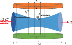
Figure 1. A simplified configuration of the Li-Baker detector for the EMR detection of a HFGW [56]. Here, the HFGW is assumed to pass through the static magnetic field along the z-axis. A Gaussian beam (the blue region) is applied in the same direction and the generated transverse first-order PPF signal is detected by a single-photon detector located at the waist of the Gaussian beam.

Download figure:
Standard image High-resolution imageWithout loss of the generality, we assume that a modulated Gaussian beam:

is applied to the static magnetic field along the z-axis direction [45]. Here, with W0 being the waist radius of the Gaussian beam, and , , . Also, λe , κe , , and δ are the wavelength, wave vector, center frequency, the Rayleigh length, and the phase factor of the Gaussian beam, respectively. In this work, we specifically take that [33, 57], (the corresponding power of the used laser is about 10 W), , and . The high stationary magnetic field is assumed to be distributed in the region: , with [45]. Formally, a modulated function is introduced to extend the detection bandwidth, wherein the modulated parameter is taken as: and β = 5.0. The spectral distribution of the modulated Gaussian beam is shown in figure 2, which means that the GW whose frequency is within the range: Hz might be detected.


![$z = [-l_1,l_2]$](https://content.cld.iop.org/journals/1367-2630/26/5/053015/revision2/njpad4204ieqn15.gif)


Figure 2. The normalized spectrum of the applied modulated Gaussian beam, which indicates that the detectable bandwidth of the GWs is Hz, centered at Hz.


Download figure:
Standard image High-resolution image2.1. First-order transverse PPF signals
Physically, the applied Gaussian beam, which is along the z-direction with the electric field being , is also a strong background noise source. Therefore, to avoid such a strong background noise, we perfectly detect the transverse EMRs (e.g. along the x-direction) of the passing HFGWs (whose transports are assumed to be along the z-direction), given the z-direction electric field of the applied Gaussian beam, i.e. . This implies that if the detectors are set at the directions, whose photon receiving faces are parallel to the yz places, then the z-direction applied Gaussian beam itself (except its scattering along the other directions) could not be coupled to the detector. Therefore, the transverse EMRs (along the x-direction) of the HFGWs are perfectly detected by the detectors located near the waist of the applied Gaussian beam, and the detectable signals could be calculated by solving the Einstein–Maxwell equation for the proposed configuration shown in figure 1.


In the usual TT gauge/frame, the non-zero elements of the metric of the monochromatic gravitational wave passing through the detection system reads:

with and kg , respectively, are the dimensionless amplitude and wave number of the HFGW, and c is the light velocity. By solving the relevant Einstein–Maxwell equation, the first-order perturbation electric field along the y direction can be obtained as [45]


near the waist of the applied Gaussian beam. Above, and are the y-direction electric field and the z-direction magnetic field of the applied Gaussian beam, respectively.


Strictly speaking, as the applied Gaussian beam is naturally defined in the detector proper frame (PDF), the detectable signals should be calculated by solving the Einstein–Maxwell equation in the PDF [47–49], wherein the non-zero elements of the metric of the passing HFGW alternatively reads

with is the linearized Riemann tensor. Again, we solve numerically the Einstein–Maxwell equation with the above metric for the same detection configuration and then get the time-domain PPF signals in the PDF.
![$R_{ijkl} = [h_{il,jk}+h_{jk,il}-h_{jl,ik}-h_{ik,jl}],\,i,j,k,l = 0,1,2,3$](https://content.cld.iop.org/journals/1367-2630/26/5/053015/revision2/njpad4204ieqn28.gif)
Obviously, if the frequency of the Gaussian beam equals to that of the passing HFGW, i.e. , the density of the first-order transverse PPF along the x direction can be calculated by:


Here, and are the electric fields of the first-order PPF signal and the magnetic field of the applied Gaussian beam. Correspondingly, the first-order energy flux density of the first-order PPF is along the x-direction, i.e. the transverse of the z-direction transporting HFGW. Thus, refers to the transverse first-order PPF, which is certainly related to the physical parameters such as the , and Ag , etc. Specifically, for a photon detector located at x = 0 (i.e. at the waist of the applied Gaussian beam), figure 3 shows the time-domain photon number distributions of the transverse first-order PPF signals by numerically solving the Einstein–Maxwell equation, either in the usual TT gauge/frame (blue line) or in the PDF (red line). Obviously, the signal behaviors calculated either in the usual TT gauge/frame or in PDF are almost the same (although their strengths are different), and the direct response (without any scattering), shown as the black line in figure 3, of the applied Gaussian beam (served as background noise) is negligible (as it transports along the z direction and thus its polarization is along the x-direction). Noted that the ±-sign in the vertical axis of the figure 3 refers to the positive- and negative of the x directions, respectively. As the detector is located at x = 0, the detected number for the positive x-direction photons and that for negative x-direction are the same, i.e. . Given the account rate of the current single-photon detector, which can reach GHz order, the signals are really sufficiently strong to be detected experimentally.


Figure 3. The time domain distribution of the first-order transverse PPF signals (i.e. the photon number) at x = 0 (near the waist of the applied Gaussian beam). At this point, the response of the Gaussian beam background applied along the z-direction vanishes, and the behaviors of the signals calculated in the usual TT gauge/frame (blue line) and the PDF are almost the same (although their strengths and transporting directions are different). The parameters are the same as those used in figure 2.
Download figure:
Standard image High-resolution imageConsequently, at the detection time , the photon number of the first-order PPF signals detected by the detector (located at x = 0) can be calculated as can be calculated as [45], i.e.


with t0 being the detection duration, Δs the receiving area of the detector, and are the time series of the detections.
![$t_s = kt_{0},\,k = [0,1,2, \ldots, 100]$](https://content.cld.iop.org/journals/1367-2630/26/5/053015/revision2/njpad4204ieqn36.gif)
2.2. Data generation method
As mentioned above, the behaviors of the first-order transverse PPFs calculated in either the usual TT gauge/frame or in the PDF are almost the same, although their strengths are different. Basically, the different signal strengths refer only to the choice of the signal-noise ratio (SNR) during the detected data processing. Specifically, let us first assume that the time domain signals , generated by using a photon detector with the photon receiving surface , (thus m2) [33], has been detected by the single-photon detector with the duration t0 (e.g. here). Next, the noise data should be generated, as noise is unavoidable in any signal detection. For simplicity, in the present work we only consider the Gaussian white noises (GWNs). Therefore, the simulatively detected data for the processing can be generated by superposing the signals, shown in figure 3 with the simulated GWNs [57], with the controllable SNR [58]:


Here, N is the data quantity, and are the amplitudes (i.e. photon number) of the first-order PPF signals and the added GWNs, respectively. In practice, signal detection is performed by multiple repeats, and thus these amplitudes are the accumulation of the many detection events typically such as ones. In the present work, we assume that the above data amplitudes are generated by the accumulation of 104 detected events. Each of the time-domain detected data is obtained by using the single-photon detector (located at x = 0) to detect the transverse first-order PPF signal, with the account rate being at GHz order. This is why the data amplitude in figure 4 is now sufficiently large for processing.


Figure 4. The simulated time-domain detection signals. The blue line is the pure first-order transverse PPF signal, the yellow line is the GWN, and the red line is the superposition of the pure- and noise signals with SNR = 1. Here, the frequency and dimensionless amplitude of the HFGW are Hz and , respectively. The horizontal axis represents the detector's detection time, and the vertical axis represents the magnitude of the relevant signals. Noted that, here, the data amplitude is sufficiently large, as it is accumulation of 104 time-domain detected events. The account rate of the single-photon detector, located at x = 0, is set as 1 GHz.


Download figure:
Standard image High-resolution image3. The simulated time-domain detected data processing
With the signals (i.e. the redline in figure 3) obtained by solving the Einstein–Maxwell equation in the PDF, in this section, we discuss how to extract the time-domain signals by using the single-photon detector (whose account rate is assumed to be at the GHz order), and then the simulated detected data is generated by superposing the signal data with the simulated noise data. The amplitude of each detected data is the accumulation of 104 detected events.
3.1. Data generations
The simulated time domain detection data can be generated as follows: First, we extract 101 dots from the blue line in figure 4, with s, to get a -dimension data as the pure time-domain first-order PPF signals. Here, the frequency and dimensionless amplitude of the simulatively-detected GW are set as: Hz and , respectively. Then, we add a GWN to these data with the SNR = and get a simulated 101-dimension time-domain detection data.
![$t_s = [0, t_0, 2\times t_0, \ldots, 100\times t_0]\times 10^{-9}$](https://content.cld.iop.org/journals/1367-2630/26/5/053015/revision2/njpad4204ieqn45.gif)


![$[0,1]$](https://content.cld.iop.org/journals/1367-2630/26/5/053015/revision2/njpad4204ieqn49.gif)
In our study, we aim to generate sets of simulated time-domain detection data. This total is divided into two subsets. The first subset, encompassing 8000 sets, is generated by randomly incorporating various high-frequency gravitational wave (HFGW) signals. These signals have amplitudes within the range: and frequencies within the range: Hz, this data is then combined with GWNs, featuring an SNR of , and designated as positive samples. Each data set within these positive samples is labeled as 1. The remaining 2000 sets form the second subset, composed of GWNs with varying means and variances. These sets are generated to function as negative samples, with each data set marked as 0. After normalizing both the positive- and negative samples, we disrupt them to generate the simulated time-domain detection data of sets, shown in figure 5(a). As seen in figure 5(b), the generated time-domain data is split into the training-, validation-, and the test datasets, with the ratio is set as .

![$A_g = 1.0\times[10^{-31}, 10^{-29}]$](https://content.cld.iop.org/journals/1367-2630/26/5/053015/revision2/njpad4204ieqn53.gif)
![$\omega_g = 2\pi\times[10^{8}, 10^{10}]$](https://content.cld.iop.org/journals/1367-2630/26/5/053015/revision2/njpad4204ieqn54.gif)
![$(0,1]$](https://content.cld.iop.org/journals/1367-2630/26/5/053015/revision2/njpad4204ieqn55.gif)


Figure 5. (a) The datasets of the positive samples and pure noise negative samples were randomly generated by different amplitude Ag and frequency ωg and the GWs in time-domain. Here, the vertical axis is the normalized value of the sum of the simulated time-domain detection data at different detection time ts ; (b) the training-, validation- and test datasets of the simulative time-domain detection data.
Download figure:
Standard image High-resolution image3.2. CNN model and data classification
We use a two-class CNN model, whose structure and the relevant parameters are shown in table 1, to calibrate the positive sample data. Generally, a CNN model mainly contains the convolution-, ReLU-, maxpooling-, flatten-, linear-, dropout- and softmax layers. Various layers are incorporated within a CNN model, each serving a unique purpose. Convolutional layers are responsible for feature extraction, employing filters that discern patterns within the data. Rectified Linear Units or ReLU layers infuse non-linearity into the model, preserving positive values and eliminating negative values from the convolution output. The complexity of the model is reduced by Max pooling layers, which downscale the dimensions of the input data, retaining only the maximum values from segments of the input. Finally, the output of the trained model can be used to identify if the input dimension data is the positive sample one or not.

Table 1. CNN model structure.
| Layer (type) | Output shape | Param |
|---|---|---|
| Input | (None, 1, 101, 1) | 0 |
| convolution | (None, 1, 101, 8) | 24 |
| ReLU | (None, 1, 101, 8) | 0 |
| MaxPooling | (None, 1, 51, 8) | 0 |
| convolution | (None, 1, 51, 16) | 272 |
| ReLU | (None, 1, 51, 16) | 0 |
| MaxPooling | (None, 1, 26, 16) | 0 |
| convolution | (None, 1, 26, 32) | 1056 |
| Relu | (None, 1, 26, 32) | 0 |
| MaxPooling | (None, 1, 7, 32) | 0 |
| Dropout | (None, 1, 7, 32) | 0 |
| convolution | (None, 1, 7, 64) | 4160 |
| Relu | (None, 1, 7, 64) | 0 |
| MaxPooling | (None, 1, 2, 64) | 0 |
| Dropout | (None, 1, 2, 64) | 0 |
| Flatten | (None, 128) | 0 |
| Linear | (None, 32) | 4128 |
| Relu | (None, 32) | 0 |
| Softmax | (None, 2) | 0 |
During the training, we add a L2-regularization proceeding and the dropout layer to prevent overfitting. Here, L2-regularization is realized by adding a L2 norm, with the weight λ into the loss function, as its penalty term; the dropout layer is used to temporarily discard certain units from the neural network with certain probabilities. With the CNN architecture shown in table 1, in what follows, we use Tensorflow [59] (see, e.g. www.tensorflow.org) to build the CNN model and then implement the train on the above-mentioned spatial domain training set. By changing the hyperparameters to compare the performance of the trained models, one can optimize the relevant hyperparameters. In the present work, the optimized hyperparameter of the L2-regularization can be obtained after the tuning as λ = 0.01, which implies that the probability of temporarily discarding units is optimized to 0.3. Similarly, the training times (i.e. epochs), the learning rate of Adam optimizer (called lr), and the BatchSize (i.e. the number of training data bars) can also be optimized to the desired values; typically, e.g. epochs = 100, lr = 0.001, and BatchSize = 128. After these hyperparameter optimizations, highly accurate training can be realized. The CNN architecture can be used to train a new CNN model with the datasets in the simulated time-domain detection data generated above. It is shown in figure 6(a) that the accuracies of both the training- and validation sets can reach to 95%, and the loss is decreased to 0.18. This represents that the CNN training model used has sufficiently high accuracies on both the training- and validating sets. Using such a trained CNN model to the test dataset, we get the ROC curve shown in figure 6(b) with the AUC being 0.986, which is very close to the optimal value 1.

Figure 6. (a) The training result obtained by using the CNN model for the simulated time-domain detection data. It is shown that the accuracy is approaching , and the loss is close to 0.2; (b) the ROC curve for the simulated time-domain detection with the AUC being calculated as 0.986.

Download figure:
Standard image High-resolution imageWith the above CNN model, we now develop the data; the frequency and dimensionless amplitude of the inputting HFGWs are assumed as Hz and , respectively. The original positive samples with 3000 data are obtained by the pure first-order PPF signal superposed by the GWNs with SNR = 1. The GWNs also generate the negative samples with 2000 data. Then, the simulated detection databases (with a total of 5000 samples) can be obtained by mixing the above positive- and negative samples, which are typically shown in figure 7(a), wherein the dimensions of each data are . Following this, we apply the previously validated, trained CNN model to analyze a 5000-group sample dataset. From this analysis, we successfully identify 3517 instances of effective positive samples. In this case, 2000 data are stochastically selected as the positive sample signals, as shown in figure 7(b). They will be further processed to extract the information of the simulatively detected HFGWs.


Figure 7. (a) A time-domain detection database for the simulatively detection of the HFGW, whose frequency and amplitude are assumed as Hz and , respectively. The original positive (negative) sample data (the dimensions of each data are ) are represented by the blue (red) points. (b) The positive sample signals are stochastically selected from the effective positive sample data, which is obtained from the time-domain detection databases by using the CNN identifications. Here, the horizontal axis is the mean of the GWNs, and the vertical axis represents the standard deviation of the GWNs.


Download figure:
Standard image High-resolution image3.3. Comparison with various classification algorithms
Certainly, many algorithms can be used to implement the expected data classification. We now compared the performance of the CNN model demonstrated above with the other classifiers, typically such as the K-nearest neighbor (KNN) [60], random forest (RF) [61], support vector machines (SVM) [62], naive Bayes classification (NB) [63] and logistic regression (LR) [64] algorithms, etc. For the comparison, we use the same test and training sets generated in section 3.1, and then run the different algorithm for the classification. The accuracies using different algorithms are listed in figure 8. It is seen that, compared with the other machine learning algorithms, the accuracy of the used CNN model is higher than that of the other algorithm by about 10%.

Figure 8. Accuracy comparison between the CNN model and the other machine learning algorithm, with the same data set.
Download figure:
Standard image High-resolution imageWe now discuss the possible improvements by using the trained model, compared with the usual matched filtering algorithm without the CNN pre-processing. Given that the matched filtering algorithm requires significantly powerful computing power and relatively long processing times, we simply use the Pearson correlation coefficient, defined by equation (8), to quantify the correlation between the same two vectors. It is shown in figure 9 that, compared with the usual matched filtering algorithm, the execution time of the CNN is shorted by almost two orders. However, the classification accuracy is almost the same.

Figure 9. The ROC curve and execution time comparisons between the CNN model and the usual matched filter algorithm, with the same data set.
Download figure:
Standard image High-resolution image4. Extracting the typical parameters of the simulative detected HFGWs by template matchings
With the positive sample signals shown in figure 7(b), obtained by the above deep learning on the simulated time-domain detection data, we now discuss how to extract the physical parameters of the simulatively detected HFGWs. This can be achieved by using the well-known template matching technique. Basically, the estimations of certain parameters from big data can be implemented by comparing them with the data in the relevant template library one by one. Here, we use the time-domain positive sample data obtained by the above CNN model to match the template library, which is generated by only the pure time-domain transverse PPF signals. The parameters in the pure transverse PPF signals are used to estimate the ones with the largest correlation positive sample data.
4.1. Frequency information
Firstly, we discuss how to extract the frequency information of the simulatively detected HFGWs from the classified time-domain detection data shown in figure 10(b) by using the frequency matchings. Suppose that the frequency of the simulatively detected HFGW is in the range of Hz and the dimensionless amplitude is , we get the template library data by using equation (6) to generate 2000 data (their frequency difference is the same) of the pure first-order transverse PPF signals (without any noise). Figure 10 shows the established frequency template library, wherein each data set has a defined frequency label and each point represents template data, whose dimension is also set as .
![$\omega_{g} = 2\pi\times[0.84, 1.16]\times10^{9}$](https://content.cld.iop.org/journals/1367-2630/26/5/053015/revision2/njpad4204ieqn66.gif)


Figure 10. A frequency template library of the first-order transverse PPF signals, wherein the frequency parameters of HFGWs are set as in the range: Hz (see more clearly in figure (b) with the short frequency distance). The vertical axis is the dimensionless amplitude of the HFGWs in the frequency template library. Here, the frequency template library includes 2000 data, and the nearest frequency distance between two frequency points is set as Hz.
![$\omega_{g} = 2\pi\times[0.84, 1.16]\times 10^{9}$](https://content.cld.iop.org/journals/1367-2630/26/5/053015/revision2/njpad4204ieqn69.gif)

Download figure:
Standard image High-resolution imageIt is known that, the correlation between two vectors: and , can be described by the Pearson correlation coefficient [65]:


Here, and are the mean values of X- and Y vectors, respectively. Obviously, the value range of this coefficient is: ; the larger the value of r corresponds, the higher the matching degree, and thus r = 1 means the perfect matching. On the contrary, represents the mismatch of the two vectors, and means that the two vectors are negatively correlated (i.e. their parameters are completely independent).


![$r\epsilon [-1,1]$](https://content.cld.iop.org/journals/1367-2630/26/5/053015/revision2/njpad4204ieqn75.gif)


By matching each data in the positive sample database with the data in the frequency template library shown in figure 10 (with also data) one by one, the frequencies corresponding to the largest Pearson correlation coefficients are output as the estimated frequencies of the simulatively detected HFGWs. It is seen from figure 11 that the estimated frequencies reveal a statistical distribution, which can be fitted as a Gaussian curve (i.e. the red line in figure 11). The vertical axis in figure 11 represents the number of positive sample data.


Figure 11. The statistical distribution of the estimated frequencies, obtained by matching the positive sample data (generated by the simulation detection of the HFGW with the frequency Hz) with the frequency template library (generated by the noise-free simulative detections of the HFGWs, whose frequencies are set as in the range: Hz. The red line is the fitted Gaussian distribution curve.


Download figure:
Standard image High-resolution imageThe accuracy of the above frequency parameter estimations is described below. According to the central limit theorem [66], the errors deviate stochastically from their average value. Therefore, the confidence level of the estimation is defined as the probability that the estimated value of the parameter falls in the corresponding area [67]. The confidence interval [67] refers to the error range between the sample statistical value and the overall parameter value at a certain confidence level. Of course, a larger confidence interval means a higher confidence level. From the statistical distribution shown in figure 11, we argue that the mean value of the estimated frequency is Hz, which is the same as the input frequency: Hz of the simulatively detected HFGW. The standard deviation is calculated as: Hz. With the present 2000 sample amounts, the confidence interval in: (, ) = Hz, with the variance multiple z = 1.96 [67] (describing the degree of deviation from the variance) at 95% confidence level can be obtained.


4.2. Dimensionless amplitude information
Continuously, we discuss how to extract the dimensionless amplitude of the simulatively detected HFGWs from the positive samples shown in figure 7(b). Similarly, we first generate the amplitude template library of the HFGWs wanted to be detected. It is seen from equation (7) that the amplitude of the input GW is linearly related to the amplitude of the first-order PPF signal without noise. Given that the frequency information of the simulatively detected HFGWs had been extracted by the above frequency matchings, the amplitude template library can be generated simply as follows. Inputting a series of HFGWs with different dimensionless amplitudes but the same frequency (i.e. the mean value of the estimated frequency by the above frequency matchings), a series of the noise-free first-order transverse PPF signals generated simulatively are served as the amplitude templates library. Here, the amplitudes of the input HFGWs are selected as in the range: with the step being . Figure 12 shows specifically the template data of the simulatively detected HFGW (with the estimated frequency: ), whose dimensionless amplitudes are assumed to be in the range: . In the figure, each point represents a template data with the dimensions being .

![$A_g = [10^{-32}, 10^{-28}]$](https://content.cld.iop.org/journals/1367-2630/26/5/053015/revision2/njpad4204ieqn88.gif)


![$[10^{-32}, 10^{-28}]$](https://content.cld.iop.org/journals/1367-2630/26/5/053015/revision2/njpad4204ieqn91.gif)


Figure 12. The dimensionless amplitude template library of the simulatively detected HFGW with the frequency Hz. Here, the horizontal axis is the possible amplitude in the range: , each of them generated a template data in the amplitude template library. The vertical axis represents the frequency of the HFGWs in the amplitude template library. Figure (b) is the enlarged version of the figure (a) for the shorter amplitude distance. The dimensionless amplitude template library includes 10 000 data, and the nearest amplitude distance between two points is set as .

![$A_{g} = [10^{-32}, 10^{-28}]$](https://content.cld.iop.org/journals/1367-2630/26/5/053015/revision2/njpad4204ieqn94.gif)

Download figure:
Standard image High-resolution imageDifferent from the Pearson correlation coefficients used above for the frequency matching, the amplitude information can be extracted simply by calculating the amplitude data correlation between the positive sample data and the template data. This is measured by the Euclidean distance [68]:

between the vector in the positive sample and the vector in the template. Certainly, the smaller the Euclidean distance corresponds, the greater the magnitude correlation. To this end, we match each data in the positive sample database with the amplitude template library one by one. Alternatively, a set of template data with the smallest Euclidean distances is treated as the possible amplitude values of the simulatively detected HFGWs. The matched results are also shown as a statistical distribution, shown schematically in figure 13. Here, the horizontal axis represents the output matching amplitudes, and the value on the vertical axis is the number of the positive sample data whose amplitudes fall in the amplitude range of the corresponding histograms. Again, the estimated amplitudes can also be fitted as a Gaussian curve, shown as the red line in figure 13. It shows that the mean value of the estimated amplitudes is: , which is very close to the input value: , with the standard deviation being . The confidence level of such an estimation is at 95% in the confidence interval: .


Figure 13. The dimensionless amplitude distribution obtained by the matchings between the positive signal with the amplitude template library. The red line is the fitted Gaussian distribution curve.
Download figure:
Standard image High-resolution image4.3. Multi-data testings
The reliability of the data processing method presented above could be tested by using multiple datasets for the different simulative detections.
In fact, much detection data can be simulatively generated for the different parameters of the HFGWs, as well as the background noises. For example, for the simulative detecting of the HFGWs, whose frequencies are in the range Hz and the dimensionless amplitudes are in the range , we can specifically generate the simulative test dataset shown in figure 14(a). The ROC curve of the trained CNN model to identify the positive samples with the test dataset is shown in figure 14(b), with the AUC being 0.978. One can see again that the trained CNN model possesses a sufficiently high resolution to identify whether the test dataset contains the HFGW signals accurately. Thus, the parameter estimation for the simulatively detected HFGWs is significatively accurate.
![$\omega_g = 2\pi\times [10^8, 10^{12}]$](https://content.cld.iop.org/journals/1367-2630/26/5/053015/revision2/njpad4204ieqn102.gif)
![$A_g = 1.0\times[10^{-33}, 10^{-29}]$](https://content.cld.iop.org/journals/1367-2630/26/5/053015/revision2/njpad4204ieqn103.gif)
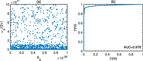
Figure 14. (a) The test set with the positive samples for the frequency band: Hz, and that of the amplitudes: ; (b) the test AUC curve of the CNN model on the test set with the ROC being 0.978.
![$\omega_g = 2\pi\times[10^8,10^{12}] $](https://content.cld.iop.org/journals/1367-2630/26/5/053015/revision2/njpad4204ieqn104.gif)
![$A_g = [10^{-33}, 10^{-29}]$](https://content.cld.iop.org/journals/1367-2630/26/5/053015/revision2/njpad4204ieqn105.gif)
Download figure:
Standard image High-resolution imageCertainly, for the input of any HFGW signal, the corresponding positive samples (containing the HFGW-induced first-order PPF signals) with 2000 or more groups of data can be obtained. By matching them with the data in the corresponding frequency- and amplitude template libraries, the confidence interval of amplitude and frequency in the HFGW signals can be effectively estimated. In table 2, we also list a series of estimated results at confidence level. This indicates that the proposed data processing method, based on deep learning, is feasible for the practice EMR detections of the HFGWs.

Table 2. Multi-data testings to extract the parameters of the simulatively detected HFGWs.
| Frequency estimations | Amplitude estimations | ||
|---|---|---|---|
| ωg ( Hz) | The confidence interval at 95% confidence level | Ag | The confidence interval at confidence level |


5. Discussions and conclusions
Based on the development of the Li-Baker detector, we developed a deep learning method to process the raw detection data for the simulative EMR detections of HFGWs. The detected data is generated by calculating the first-order transverse EMRs of the simulatively detected HFGWs in the strong GWN background. Specifically, a robust CNN model has been proposed to identify the generated detected data, at significantly high accuracy, from the simulated raw detection data. Consequently, the typical parameters, such as the frequency and dimensionless amplitude, of the simulatively detected HFGW can be effectively estimated by matching the obtained positive samples with the relevant template libraries. The confidence level of the parameter estimations can reach 95% in the corresponding confidence interval.
In principle, the accuracies of the CNN model and the estimated parameters can be further improved by using stronger computing resources to generate bigger detection data and the matched template library. Although the noises simulatively treated here are limited to the most typical GWNs, the proposed method could be developed to process the other noises. Indeed, the noise of the realistic detectors is very complicated. Also, in the present work, we only consider the simulative detections of the typical HFGWs with a given frequency and amplitude. However, most of the HFGWs are stochastic ones without the defined waveforms. Therefore, it is necessary to develop possible new data processing methods by deep learning to process the EMR detection data for stochastic HFGW detection. Novel techniques for relevant big data processing might be developed using Bayesian statistics. Also, the physical parameters of the stochastic HFGWs could be estimated by using the cross-correlation between the data obtained by the multiple detectors. Finally, we have only discussed the simulative detection by using the x-direction detectors located at x = 0, near the waist of the applied Gaussian beam. At this point, the behaviors of the transverse first-order PPF signals are relatively simple and the zero-order responses of the applied Gaussian beam (i.e. the strongest background noise) can be safely neglected. For the more general configurations, solving the Einstein–Maxwell equation in the PDF to get the detectable first-order transverse PPF signals is relatively complicated. As a consequence, the more effective method to process the data detected by the other detected configurations with the more complicated noise behaviors still needs to be solved.
Acknowledgments
This work was supported in part by the National Natural Science Foundation of China, Nos. 11974290, 11873001 and 12347101.
Data availability statement
All data that support the findings of this study are included within the article (and any supplementary files).