


Abstract
We report the spectroscopic characterization of a Kerr parametric oscillator (KPO) based on the measurement of its reflection coefficient under a two-photon drive induced by flux modulation. The measured reflection spectra show good agreement with numerical simulations in terms of their dependence on the two-photon drive amplitude. The spectra can be interpreted as changes in system's eigenenergies, transition matrix elements, and the population of the eigenstates, although the linewidth of the resonance structure is not fully explained. We also show that the drive-amplitude dependence of the spectra can be explained analytically by using the concepts of Rabi splitting and the Stark shift. By comparing the experimentally obtained spectra with theory, we show that the two-photon drive amplitude at the device can be precisely determined, which is important for the application of KPOs in quantum information processing.
Export citation and abstract BibTeX RIS

Original content from this work may be used under the terms of the Creative Commons Attribution 4.0 license. Any further distribution of this work must maintain attribution to the author(s) and the title of the work, journal citation and DOI.
1. Introduction
Dressed states formed in a driven quantum system are typically characterized by spectroscopic measurements. For example, if a two-level system is driven on resonance, the Mollow triplet [1] is observed due to the Rabi splitting of the two energy levels hybridized with the photon number states. If, on the other hand, the drive is far detuned, the shift of the energy level due to the Autler–Townes effect, namely, the ac Stark effect [2] is observed.
The experiments originally done in atomic system have not only been reproduced, but also extended to an unexplored parameter regime using superconducting artificial atoms, referred to as a circuit quantum electrodynamics (c-QED) system [3, 4]. For example, the ac Stark shift in a c-QED system was first reported in [5], and extended to the strong dispersive regime, where it is possible to determine the population of each photon number state in the resonator coupled to the qubit [6].
Compared to the experiments using one-photon drive, spectroscopy of a two-photon driven system has been relatively unexplored in c-QED systems. The two-photon drive plays an essential role in a device called a Kerr parametric oscillator (KPO) [7, 8], which has been attracting attention for applications in quantum information processing, such as quantum annealing [9, 10] and gate-model quantum computing [11–13]. KPOs are parametric oscillators, in which the Kerr nonlinearity is larger than the photon loss rate, particularly in the single-photon Kerr regime [14]. The KPOs can be implemented using Josephson parametric oscillators [15–19] or charge-driven transmons with a superconducting nonlinear asymmetric inductive element (SNAIL) [20–22]. In both cases, an external field nearly twice the resonance frequency of the KPOs is used for parametric pumping and works as the two-photon drive.
Spectroscopic measurement for studying the energy-level structure up to the tenth excited states of the KPO of charge-driven transmons has been reported by Frattini et al [21]. By measuring the excitation energy from the ground states as a function of the two-photon drive amplitude, they revealed the crossover from a nondegenerate spectrum to a pairwise kissing spectrum formed by two excited states in the double-well meta potential of the KPO, which leads to a staircase pattern in the coherent state lifetime. This type of spectroscopic measurement for revealing the energy spectra of KPOs is important not only for understanding its fundamental physics, but also for its application to quantum information processing. For example, in [23], a gate operation of the cat qubit using excited energy levels was proposed. Moreover, a comparison of the spectroscopic measurement with the theory generally gives the calibration of the drive amplitude at the quantum chip [5, 24, 25]. This is particularly important in KPOs for precisely determining the two-photon drive amplitude to create an optimal schedule to generate Schrödinger's cat state in a short time [13, 26, 27].
Some of the authors of the present study theoretically proposed an alternative method of spectroscopy for revealing the energy level structure of a KPO under two-photon drive [28]. The method is based on the measurement of reflection coefficient of the KPO and is simpler than that used in previous studies [21, 22] because it is only performed by continuous wave measurement without using microwave pulses. In the present paper, we experimentally demonstrate the proposed method by performing reflectometry measurements of the KPO under the two-photon drive induced by the flux modulation. We compare the results with numerical simulations on the basis of the theory to interpret the experimental data. We also show that the experimental data can be used to determine the calibration of the two-photon drive amplitude, which is important for the application of KPOs in quantum information processing.
2. Device
The KPO used in this experiment is a lumped-element-type device. An optical microscope image and an equivalent circuit of the KPO are shown in figures 1(a) and (b), respectively. The left end face of the KPO is connected to a signal line via a coupling capacitor  , from which a probe signal is applied. The bottom end face is connected to a coupler for interaction with other KPOs, which are not used in this experiment. The top end face is connected to the ground plane via two Josephson junctions (JJs) and a superconducting quantum interference device (SQUID) in series, the latter of which is inductively coupled to the pump line. The JJ is placed in series with the SQUID to reduce the magnitude of the Kerr nonlinearity
  of the KPO [29]. The SQUID contains asymmetric JJs, whose critical currents are designed to be 375 nA and 625 nA, and those of the series junctions are designed to both be 1000 nA. The actual critical current of each JJ was verified by measuring the room-temperature resistance of a test structure. The KPO is placed in a dilution refrigerator and cooled to below 10 mK.
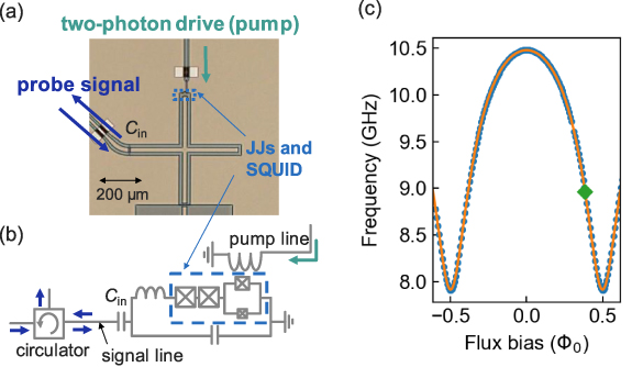
Figure 1. (a) Optical micrograph of the KPO and (b) its schematic circuit diagram. The probe signal is injected from the signal line, which is capacitively coupled with the KPO. The reflected signal is separated from the injected signal by a circulator. The two-photon drive is applied from the pump line, which is inductively coupled to the SQUID in the KPO. The DC current is also applied to the pump line to induce a static magnetic field in the SQUID loop. (c) Flux-bias dependence of the resonance frequency. The blue dots are experimental data, and the orange line shows the theoretical calculation of the resonance frequency based on the circuit model shown in (b) and fitted to the data. The green diamond represents the operation point used for the spectroscopy measurements with the two-photon drive.
Download figure:
Standard image High-resolution imageWe measure the reflection coefficient of the KPO without the two-photon drive to extract the parameters of the KPO. The reflection coefficient  is expressed by the following equation,

where  is the resonance frequency of the KPO,
  is the probe frequency, and
  (
( ) is an external (internal) loss rate. Figure 1(c) shows the flux-bias dependence of the resonance frequency. The resonance frequency of the KPO changes periodically with the flux bias induced by the DC current applied to the pump line. In the following measurement, we fix the DC flux bias to
  , where
  is the magnetic flux quantum. At this flux bias, the resonance frequency
  , the external loss rate
  and the internal loss rate
  are estimated by fitting the measured
  to equation (1). Note that the internal loss rate obtained from this reflection measurement may include the contribution from pure dephasing; the actual internal loss rate
  is related to
  as
as  , where
  is the pure dephasing rate of the KPO.
3. Measurement of reflection coefficient under two-photon drive
Next, we measure  under the two-photon drive using a vector network analyzer (VNA). The two-photon drive generated by an additional microwave source at room temperature is applied to the pump line on the chip (figure 1(b)). The frequency of the two-photon drive
  is approximately twice the resonance frequency of the KPO, and the detuning is defined as the difference between the resonance frequency and half of the two-photon-drive frequency, that is,
  .
.
The Hamiltonian of the KPO in a frame rotating at  is expressed as [17]

where  is the photon annihilation operator, and
  is the amplitude of the two-photon drive. The Kerr nonlinearity
  is determined by measuring the probe-power dependence of
  [16]. The Fock state
  , where
  is the photon number, is the eigenstate with eigenenergy of
  when the two-photon drive is absent. To examine situations with varying degeneracy of eigenstates, we use three different
  ;
; 
 , where
  is the total photon loss rate. If
  , the Fock states
  and
and  (
( ) are degenerate at
  . In the case of
  , there are no degenerate states at
  .
.
Figure 2 shows the amplitude of  as a function of
  and the two-photon drive power at the generator output
  for different detunings [(a)
 , (b)
, (b) , (c)
, (c) ]. Here,
  was changed for each scan of
  using the VNA. In all cases, we observed single dips in
  corresponding to the transition from the state
  to the state
  for sufficiently small
  . As
. As  is increased, the spectra exhibit other transitions, and the patterns and the number of transitions [6, 2, and 3 for (a), (b), and (c), respectively] vary with the detuning. In addition, amplification peaks (
 ) are observed in figures 2(a) and (c), while they are absent in figure 2(b). For
  , the transition observed at
  is an absorption dip at small
  and splits into two amplification peaks as
  is increased. In the region of
  , three of the six transitions shift toward higher frequency, and the others toward lower frequency as
  is increased. For
  , two transitions are observed, and the frequency of the transition observed at
  is constant and that of the other transition becomes lower in frequency as
  is increased. For
  , one of the three transitions is observed as an amplification peak, and the others are absorption dips. One of the absorption dips shifts toward higher frequency, and the other toward lower frequency as
  is increased.

Figure 2. Amplitude of reflection coefficient as a function of the probe frequency  and the two-photon drive power
  with different detunings of (a)
  , (b)
, (b)  , and (c)
  . The power of the two-photon drive
  is defined as that at the output of the signal generator.
Download figure:
Standard image High-resolution image4. Numerical simulations
We numerically simulate the reflection coefficient for comparison with the experiments. The experimentally determined frequency detuning  , Kerr nonlinearity
  , and internal (external) photon loss rate
  (
( ) were used for the simulations. The calculations are performed using Python and QuTiP package [30, 31]. The reflection coefficients are calculated following [28] as

with

Here,  is the contribution of the transition from the state
  to the state
  in the reflection coefficient. The state
  is the energy eigenstate of the KPO, and the state is labeled by the photon number of the state when the two-photon drive is absent. Here,
  is the transition frequency from the state
  to the state
  calculated by diagonalizing the Hamiltonian equation (2).
  is the
  th diagonal element
  of the steady-state density matrix obtained by solving a Gorini–Kossakowski–Sudarshan–Lindblad (GKSL) master equation with a single-photon loss. Here,
  is used as the single-photon loss rate.
  is the matrix element of the one-photon transition, and
  is the expectation value of the photon number for the state
  . Fock states with a photon number up to 30 are considered in the calculation.
Figures 3(a)–(c) show the result of the numerical simulations, which are qualitatively in agreement with the experimental results shown in figures 2(a)–(c). For quantitative comparison in the following sections, here we convert the horizontal axes in figure 2, the power of the two-photon drive  , into the amplitude of the two-photon drive
  , which can be calculated by the first-order derivative of resonance frequency with respect to the current applied to the pump line
  (appendix


Figure 3. Simulated amplitude of reflection coefficient as a function of the probe frequency  and the amplitude of the two-photon drive
  with a detuning of (a)
  , (b)
, (b)  , and (c)
  . (d)–(f) Spectra in figure 2 replotted as a function of
  in the horizontal axis. (g)–(i) Energy of the eigenstates, (j)–(l) population of the energy eigenstates for the steady state calculated by a GKSL master equation, and (m)–(o) matrix elements of the one-photon transition as a function of two-photon drive amplitude
  with a different detuning of
  (g), (j) and (m),
  (h), (k) and (n), and
  (i), (l) and (o). Gray dashed lines in (d)–(f) represent the transition frequencies calculated from eigenenergies shown in (g)–(i), respectively. Attenuations in the pump line
  were determined to be (d) −57.0 dB, (e) −57.6 dB, and (f) −57.6 dB to minimize the square of the difference between the measured and calculated transition frequencies.
Download figure:
Standard image High-resolution imageFrom the measurement results shown in figure 1(c), we obtained  at this bias point. Another parameter, the two-photon drive power at the chip
  , is
, is  , where
  is the attenuation of the two-photon drive inside and outside the refrigerator. The attenuation
  is estimated by comparing the measured transition frequencies with the theoretical ones, which were calculated using the Hamiltonian in the absence of a coherent drive under the rotating wave approximation. If a transition frequency is separated from others by a frequency larger than the line width, the transition frequency is extracted from the measured spectrum (figures 2(a)–(c)) by fitting it to the following equation [28]
where  and
and  correspond to nominal external and internal loss rates, respectively. To extract
  , we used
  as a fitting parameter minimizing the square of the difference between the measured and calculated transition frequencies. The estimated values of
  are −57.0 dB, −57.6 dB, and −57.6 dB with ±0.1 dB uncertainties for
  respectively. From an independent measurement using a chip with a through transmission line, we estimate that the two-photon drive is attenuated by 58 dB from the microwave source to the KPO with an accuracy of ±2 dB, which is consistent with the above result.
Figures 3(d)–(f) show the same experimental data as figure 2 plotted as a function of  in the horizontal axis. The theoretical calculation of the transition frequencies
  's is also plotted by gray dashed lines. The measured frequencies agree with the calculated transition frequencies within the error of 0.90 MHz, 0.29 MHz, 0.95 MHz for
  respectively.
5. Interpretation of transition spectra
The experimental results (figures 3(d)–(f)) are highly consistent with the numerical calculations (figures 3(a)–(c)). The agreement indicates that the theoretically predicted energy levels and the population distribution of the stationary state are reproduced in the experiment. From here, we interpret each transition spectrum shown in figures 3(a)–(c). Note that the two-photon drive does not change the photon number parity, whereas the one-photon drive used as the probe signal does. Therefore, transitions can occur between the states  and
and  , where both
  and
and  are non-negative integers. For the transitions
  at
at  to be visible, both
  and
and  must be non-zero (equation (4)). Whether the transition at
  appears as a peak or dip in the spectrum is determined by the sign of the population difference
  . Thus, the reflection measurement provides information about the eigenenergy, population distribution, and transition matrix element.
First, we consider  . Figures 3(g) and (j) show the numerically calculated energy levels and their populations, respectively, for the four highest energy eigenstates of the KPO in the rotating frame as a function of
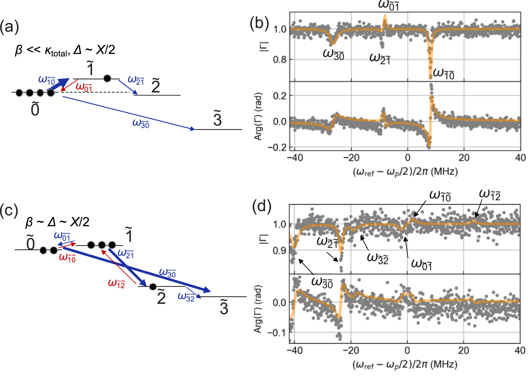
  . The energy level and the state population are schematically drawn in figures 4(a) and (c). In the case of
  (figure 4(a)), the states
  and
and  are almost degenerate. Because
  is sufficiently smaller than
  , the population is concentrated in the state
  . Therefore, the transition
  (
( ) should appear as an absorption dip (amplification peak). Figure 4(b) plots both experimentally obtained and numerically calculated
  's as a function of
  . As expected, we observe an absorption dip at
  and a small amplification peak at
  and their difference in magnitude comes from the difference in their transition matrix elements of the one-photon drive. Similarly, the transitions at
  and
and  appear as absorption dips. The fact that the transition between the states
  and
and  exhibit weak probe power indicates that at least one of them deviates from the Fock states. We note that the discrepancy observed for the dip at
  is possibly due to its proximity to the peak at
  . As discussed in [28], when two transitions are close to each other, there is an interference effect, which is neglected in equations (3) and (4).

Figure 4. Schematic energy diagram and the reflection coefficient as a function of the probe frequency for  (a), (b) and
  (c), (d). In (a) and (c), the black dots in each energy levels represent the population of the corresponding state. Blue (red) arrows in the energy diagrams represent the transitions from the state with larger (smaller) population to the state with smaller (larger) population, which results in the absorption dips (amplification peaks) in
  . Thickness of the arrows qualitatively represents the strength of the transition. In (b) and (d), gray dots represent the experimental data, while the solid orange curves represent the numerical simulations.
Download figure:
Standard image High-resolution imageFigures 4(c) and (d) show the schematic energy diagram and the reflection coefficient at  , respectively. Because the population inversion (
 ) is created, the transition
  at
at  turns out to be an amplification peak, which is referred to as dressed-state amplification [32]. Because the degeneracy of the states
  and
and  is lifted at
  (figure 3(g)), the transition
  is separated from the transition
  and becomes visible as another amplification peak at
  . The transition
  is separated from the transition
  and also becomes visible as another dip at
  . Because four states
  ,
,  ,
,  , and
, and  are involved, there are eight possible transitions
  ,
,  ,
,  , and
, and  , which appear as four absorption dips and four amplification peaks. However, the transitions
  and
and  cannot be observed because the matrix element of the one-photon transition
  and
and  are too small as shown in figure 3(m). This makes the number of transitions six. Signal-to-noise ratio in figure 4(d) is lower than that in figure 4(b). This is because the amplitudes of the peaks and dips in figure 4(d) are smaller than those in figure 4(b). The signal-to-noise ratio can be improved by increasing the average number of the VNA.
For  , some of the transitions disappear as shown in figure 3(a). The peak and dip in the transitions
  at
at  and
and  at
at  disappear because the population difference between
  and
and  is small (figure 3(j)). Similarly, the dip in the transition
  at
at  disappears because the difference between
  and
and  is small. The peak height of the transition
  at
at  becomes small due to decreasing
  (figure 3(m)).
In the case of  , the states
  and
and  are almost degenerate regardless of the value of
  as shown in figure 3(h). Within the probe frequency range in this measurement (figure 3(e)), the transitions
  and
and  can contribute to the spectrum. However, the transition
  at
at  is not visible because the matrix element of the one-photon transition
  is small (figure 3(n)). For the transitions
  , the frequencies
  and
and  are the same, so the dip at
  overlaps with the peak at
  , resulting in two distinguishable spectra. As the populations of
  and
and  approach 0.5 (figure 3(k)), the dip depth at
  appears to decrease (figures 3(b) and (e)). In contrast, although the matrix element of the one-photon transition
  slightly decreases (figure 3(n)), the peak of
  at
at  becomes more visible, because the population difference between
  and
and  increases (figure 3(k)). For
  , the steady state of the states
  and
and  are the same mixed state [10, 11].
For  , there are no degenerate states at
  (figure 3(i)). We observe one amplification peak at
  and two absorption dips at
  and
and  , which can be attributed to the relationship between the populations
  (figure 3(l)). As the population
  increases, the transition
  become more visible as the dip at
  in
in  (figures 3(c) and (f)). In the same regime, although the population difference between
  and
and  decreases, the peak at
  become visible because
  increases (figure 3(o)).
6. Analytical calculation of transition frequencies
The transition frequencies described thus far have been calculated by diagonalizing the Hamiltonian equation (2), and are in good agreement with the experimental data. As shown in appendix  can be calculated analytically when
  , in which the frequency of the two-photon drive is in resonance with the energy difference between the states
  and
and  . Namely, the frequency shifts of
  when
when  are given by
 and
and  , respectively, where the term
  is caused by the Stark shift of the state
  and the term
  results from the Rabi splitting originating from the states
  and
and  . Figure 5 shows the comparison of transition frequencies obtained from diagonalizing the Hamiltonian when
  (gray lines) and analytical formula (dashed lines). They are in good agreement for small
  . In the range of
  , the difference between them is less than 0.38 MHz, which is smaller than
  . However, a discrepancy can be seen in the range of
  especially for
  . This is because the contribution of the states with large photon numbers cannot be ignored when
  is large. Namely, the analytical formula is derived by considering only the Fock states with the photon number up to 2. However, as
  increases, the population of the Fock states with larger photon numbers increases and the states
  ,
,  , and
, and  can no longer be well approximated as
  and
and  , which are analytically derived in the subspace spanned by
  ,
,  , and
, and  (see appendix

Figure 5. Comparison of transition frequencies obtained from diagonalization of the Hamiltonian (gray solid lines) and analytical calculation for the detuning  . Analytical calculation is shown by the dark blue and dark red dashed lines, which are given by
  and
and  , respectively.
Download figure:
Standard image High-resolution image7. Comparison of nominal relaxation rates
Thus far, we have investigated the  dependence of the frequency and the amplitude of peaks and dips in
  and found good agreement between the experiment and the theory as shown in figures 3(a)–(f). However, the overall linewidth of the peaks and dips in the experiments is smaller than the theoretical as seen in the figures, where it should be noted that the color scales are all the same. To examine this difference, we investigate the nominal loss rates
  and
and  obtained by fitting the measured
  to
to  in equation (6).
By comparing equations (3) and (6), the nominal external loss rate  and internal loss rate
  are given by


In figure 6, we plot  and
and  for
for  as a function of
  . For comparison, we also plot those predicted from the model,
  and
and  (equations (7) and (8)). As shown in figure 6(a),
  agrees well with
  for all
  , except that
  differs significantly from
  in the range of
  from 0.4 MHz to 4 MHz. This deviation is due to the fact that the dips in the transitions
  at
at  and
and  at
at  overlap with each other in this pump power range (figure 3(d)), so that there is the interference effect between the transitions as mentioned earlier in figure 4(b). Although the frequency difference between
  and
and  is also small in the region of
  , the deviation is not seen because the population difference between
  and
and  makes the transition
  dominant (figure 3(j)).

Figure 6. Nominal (a) external and (b) internal photon loss rates as a function of two-photon drive amplitude at  . The dots represent the experimental data [
 and
and  ], and the dashed lines represent the calculation [
 and
and  ].
].
Download figure:
Standard image High-resolution imageIn contrast, the agreement between  and
and  is poor as shown in figure 6(b). Only
  and
and  are consistent with the theory in the limited range of
  . Overall,
  is smaller than the theoretical estimation
  , except for
  in the range of
  from 0.4 MHz to 4 MHz, where we observed deviation in
  as discussed above.
The discrepancy between  and
and  is not well understood at this time. Because the nominal external photon loss rate, which is related to the single-photon decay to the signal line, is consistent with the theory, we believe that dephasing or losses other than the single-photon loss can cause the discrepancy between
  and
and  . We do not include the phase relaxation effect in equations (4) and (6), but we found that simply including phase relaxation in the master equation by
  as the Lindblad operator does not reproduce
  . One possibility is the 1/f spectrum of flux noise [33, 34], which is not taken into account in the simulation. The phase relaxation and noise spectra will need to be further investigated in future studies.
8. Conclusion
We performed spectroscopic measurements of a KPO under the two-photon drive induced by the magnetic flux modulation and compared the results with theoretical calculations. Since we use the continuous measurement of the reflection coefficient of the KPO, our method is simpler than previous studies [21, 22] for charge-driven SNAIL transmons with pulse operations. The transition frequencies are in good agreement with the calculations after adjusting the attenuation values for the microwave transmission line, which turned out to be consistent with the results of independent measurements. We also demonstrated that some transition frequencies can be interpreted as Rabi splitting and the Stark shift and provided a simple analytical formula for them. The magnitude of the reflection coefficients is also in good agreement with the calculation, and we showed that its behavior under the two-photon drive, such as the change from the absorption dip to amplification peak, can be explained by the difference in the population between the initial and final states of the transition. These results demonstrate that the system is well characterized by the model Hamiltonian including the two-photon drive induced by the flux modulation. We also investigated the nominal loss rates and found that the external loss is in good agreement with the theoretical calculation, while the internal loss rate shows significant deviation from the theory, which still needs clarification.
The spectroscopic results have potential applications in quantum annealing machines and gate-model quantum computers. The estimation of the magnitude of the two-photon drive at the quantum chip is critical for efficient parameter scheduling [13, 26, 27]. Additionally, the accurate estimation of KPO eigenenergies are useful for gate operations of a cat qubit [23].
Acknowledgments
We thank Y Kitagawa for his assistance in the device fabrication. We also thank T Aoki, K Koshino, and Y Kano for their fruitful discussions. A part of this work was conducted at the AIST Nano-Processing Facility supported by Nanotechnology Platform Program of the Ministry of Education, Culture, Sports, Science and Technology (MEXT), Japan. The devices were fabricated in the Superconducting Quantum Circuit Fabrication Facility (Qufab) in the National Institute of Advanced Industrial Science and Technology (AIST). This paper is based on the results obtained from a Project, JPNP16007, commissioned by the New Energy and Industrial Technology Development Organization (NEDO). This work was partially supported by JST Moonshot R&D (Grant Number JPMJMS226C).
Data availability statement
The data cannot be made publicly available upon publication because no suitable repository exists for hosting data in this field of study. The data that support the findings of this study are available upon reasonable request from the authors.
Appendix A: Two-photon drive amplitude
In this appendix, we derive the formula for the amplitude of the two-photon drive applied to the KPO (equation (5)) based on its relation to the modulation amplitude of the resonance frequency.
First, we derive the relation between the amplitude of the frequency modulation  and the power of the two-photon drive. We assume the time dependence of the resonance frequency as
  , where
  is the static resonance frequency and
  is the frequency of the two-photon drive. Then,
  is related to the derivative of the resonance frequency with respect to the bias current
  as
as  , where
  is the amplitude of the ac current induced by the two-photon drive. Here, we assume that the mutual inductance between the pump line and the SQUID is frequency independent. Because the root mean square value of the current
  is
is  , the average power
  is given by
  , where
  is a characteristic impedance of the pump line. Therefore,
  (in dBm) can be written as
 ![$\bar p = 10{\log _{10}}\left[ {\frac{{{Z_0}i_{{\text{amp}}}^2 \times 1000}}{2}} \right]$](https://content.cld.iop.org/journals/1367-2630/26/4/043019/revision2/njpad3c64ieqn326.gif) , i.e.
, i.e.  , and
, and  is written as

The relation between the two-photon drive  and frequency-modulation amplitude can be determined from the Hamiltonian equation (2) in a laboratory frame,

By expanding and rearranging the right-hand side of this equation into normally ordered products, the coefficient of  becomes
  . The constant terms are the resonance frequency
  of the KPO without the two-photon drive, and the oscillating term represents the frequency modulation caused by the two-photon drive. Therefore, the frequency-modulation amplitude
  can be written as
  , which together with equation (A1) leads to equation (5).
Appendix B: Analytical calculation of frequency shifts
In this appendix, we derive formulae for four of the transition frequencies as a function of the two-photon drive amplitude  , which are discussed in section 6 and shown in figure 5. We investigate the physical meaning of the frequency shift by deriving its formula analytically.
We consider the situation where  matches the energy difference between
  and
and  . In this case, the two-photon drive acts as a resonant drive for
  and
and  and as a detuned drive for the states with two different photon numbers, e.g. for
  and
and  (figure 7(a)). It is well known that a resonant drive applied to a two-level system causes Rabi splitting and a non-resonant drive causes the Stark shift [2]; here we extend the same idea to the two-photon drive applied to the KPO.

Figure 7. Schematic energy diagram under the condition that the parametric drive frequency  is resonant to the energy difference between the states
 and
and
 . (a) Energy-level diagram in a laboratory frame. The energy level is represented by Fock states and
  is the energy difference between the
  th and
  th Fock states. The parametric drive works in two different ways; the resonant drive for the states
 and
and
 (pink arrow) and the detuned drive for the states
 and
and
 (orange arrow). (b) Energy-level diagram in a rotating frame and possible state transitions. Left: the bare KPO energy levels. Center and right: the energy levels with a photon number of
  and (
and ( ) under the two-photon drive, respectively. The resonant drive between the states
 and
and
 causes the Rabi splitting (energy levels in pink). The detuned drive between the states
 and
and
 changes the energy of the state
 (energy level in orange) by ac Stark effect. The dark blue and dark red dashed arrows represent the transitions induced by the probe signals.
Download figure:
Standard image High-resolution image
If the states with a photon number of less than 3 are considered, the Hamiltonian equation (2) is rewritten as

We decompose  as
as

where


 represents a resonant drive for
  and
and  states, and
  represents a detuned drive for
  and
and  states (figure 7(a)).
First, we focus on  . This term is described as a two-level system of
  and
and  . The diagonalization of
  yields

Here, we define  . This is analogous to the derivation of the Rabi splitting for two-level systems, which can be observed as a Mollow triplet.
Next, we focus on  . This term is described as a two-level system of
  and
and  with a detuned drive. The diagonalization of
  yields

where


Here, we define  . If the amplitude of the two-photon drive is much smaller than the Kerr nonlinearity, i.e.
  , equation (A8) is written as

Comparing equations (A6) and (A11), it can be seen that the ac Stark shift is caused by the two-photon drive. Namely, the eigenenergies of  and
and  are shifted
  and
and  , respectively. From equations (A7) and (A11),
  can be written as

This rewriting from equation (A3) to equation (A12) corresponds to the rewriting of the Fock states to the dressed states shown as the orange and pink levels in figure 7(b), which are induced by the two-photon drive shown by the vertical arrows in their corresponding colors in figure 7(a).
Transition frequencies between the dressed states can be calculated from figure 7(b). Namely, frequencies for the transitions  (dark blue dashed arrows) are
  and those for the transitions
  (dark red dashed arrows) are
  . They are plotted in figure 5 in their corresponding colors.