


Abstract
Semiconducting nanowires with strong Rashba spin–orbit coupling in the proximity with a superconductor and under a strong Zeeman field can potentially manifest Majorana zero modes (MZMs) at their edges and are a topical candidate for topological superconductivity. However, protocols for their detection based on the local and the non-local conductance spectroscopy have been subject to intense scrutiny. In this work, by taking current experimental setups into account, we detail mathematical ideas related to the entanglement entropy and the fermion parity fluctuations to faithfully distinguish between true MZMs and trivial quasi-MZMs. We demonstrate that the disconnected entanglement entropy, derived from the von Neumann entanglement entropy, provides a distinct and robust signature of the topological phase transition which is immune to system parameters, size and disorders. In order to understand the entanglement entropy of the Rashba nanowire system, we establish its connection to a model of interacting spinfull Kitaev chains. Moreover, we relate the entanglement entropy to the fermionic parity fluctuation, and show that it behaves concordantly with entanglement entropy, hence making it a suitable metric for the detection of MZMs. In connection with the topological gap protocol that is based on the conductance spectra, the aforesaid metrics can reliably point toward the topological transitions even in realistic setups.
Export citation and abstract BibTeX RIS

Original content from this work may be used under the terms of the Creative Commons Attribution 4.0 license. Any further distribution of this work must maintain attribution to the author(s) and the title of the work, journal citation and DOI.
1. Introduction
Majorana zero modes (MZMs) [1–4] in condensed matter systems have been a crucial talking point, tending to their exotic attributes, such as non-Abelian quantum statistics, which maybe leveraged for futuristic quantum technologies like fault-tolerant topological quantum computation [5]. Semiconductor–superconductor heterostructures composed of Rashba nanowires proximitised with superconductors are a prime solid-state candidate for realizing MZMs [1–4, 6]. Howbeit, conclusive and unambiguous detection of MZMs in these systems has been a matter of intense scrutiny and open deliberation due to controversies involving non-topological origins of MZM-like signatures. Major experimental efforts for the detection MZMs have been based on observing zero-bias conductance peaks (ZBCPs) in the local differential conductance of normal-topological superconductor (N-TS) setups [7–12]. However, disorder-induced near zero-energy Andreev bound states (ABS), often known as quasi-MZMs, imitate local conductance signatures of MZMs to a great extent [13–21], rendering ZBCP based detection of MZMs ambiguous.
Recent protocols have thus focused on exploiting the non-locality of MZMs through non-local transport spectroscopy using the normal metal-topological superconductor-normal metal (N-TS-N) hybrid setups [6, 22–28]. The non-local differential conductance probes the bulk-gap closing and reopening and is presumed to be uninfluenced by the trivial modes [23]. Ideas proposing measurements of the full conductance matrix, which includes both local and non-local measurements, to identify topological regimes have also been presented [29, 30]. Nonetheless, numerical [28, 31] and experimental [25] studies have portrayed several issues with the non-local conductance signatures as well, with the signals becoming faint and sputtered [28] accompanied by a premature gap closing [25, 31] in the presence of disorders. This motivates exploring other possibilities that exploit non-local correlations to classify topological orders. One such attribute which can be leveraged to ascertain non-locality in topological phases [32–34] is the degree of entanglement in the system, which may be quantified using metrics derived from the von Neumann entropy, such as the disconnected entanglement entropy (DEE) [31].
In this work, we provide an in-depth analysis of various entanglement entropy signatures of MZMs in SM-SC heterostructures. We illustrate that the DEE [35] distills out the topological contributions of  units to the entanglement entropy [35–37] and is hence apt for identifying topological phase transitions, unlike the bipartite entanglement entropy (BEE) which is padded with volume and area contributions [31, 38]. In the process, we develop a new pedagogical model, 'the spinfull Kitaev chain', to elucidate the entropy signatures of
  units in Rashba nanowires from a more first-principles perspective. We demonstrate that the entanglement entropy remains robust and quantized over a wide range of controllable parameters and withstands the test of disorder and quasi-MZMs. Further, we inquire into fermion parity noise, a physical observable closely related to entanglement entropy [39]. With recent advances in the experimental measurement of fermion parity of SC-SM heterostructures [40–42], the fermion parity noise maybe potentially used for gauging entanglement entropy. We conclude by demonstrating the reliability of the DEE over the local and non-local conductance spectroscopy [31] for the conclusive detection of MZMs.
2. Methods
In this section we briefly highlight the system Hamiltonian that we consider. We then elucidate the techniques used for calculating the three major quantities presented in this paper—bi-partite and DEE, fermion parity noise, and local and nonlocal conductance.
The three terminal N-TS-N setup [25, 29, 30] that we consider is shown in figure 1(a). The setup comprises a semiconducting nanowire (in blue) with strong Rashba type spin–orbit coupling with an epitaxial layer of s-wave superconductor (in purple), placed in contact with metallic leads 'L' and 'R' (in pink). The Hamiltonian of the nanowire system in the Bogoliubov–de Gennes (BdG) representation is

where  represents the Nambu spinor, ψσ
is the electron annihilation field operator with spin
represents the Nambu spinor, ψσ
is the electron annihilation field operator with spin  and
and  represents the BdG Hamiltonian [18] described by:

Figure 1. Device schematics. (a) The N-TS-N system considered in this work. The semiconducting nanowire SM (in blue) is proximitised with a superconductor SC (in purple) which acts as a topological superconductor under a strong spin–orbit coupling and magnetic field. Two normal contacts (in pink) L and R are used to probe the TS system. (b) The pristine setup, with no disorder potential and a homogeneous on-site potential constant throughout the nanowire. (c) The disordered system where the on-site potential varies along the nanowire due to local inhomogeneities.
Download figure:
Standard image High-resolution image

where, σi
are the set of Pauli-matrices in the spin basis, with σ0 being the identity matrix and τi
are the set of Nambu-matrices in the particle-hole basis. µ is the electrochemical potential,  is the Rashba spin–orbit coupling strength,
  is the Zeeman field, B is the magnetic field and Δ is the proximity-induced superconducting gap. In this work, we elucidate two cases. First, the pristine nanowire case with
  , portrayed in figure 1(b). Here, both the superconducting gap and the on-site potential are homogeneous and constant throughout the nanowire. As stressed upon earlier, accounting for disorder is crucial for studying conclusive MZM-identification techniques. In the second case, we study the one with disorder where V(x) is non-zero and inhomogeneous. Figure 1(c) shows the disordered setup where the gap-parameter remains homogeneous but the on-site potential varies along the nanowire due to disorder-induced local inhomogeneities.
We analyze smooth inhomogeneous potentials at the ends of the nanowire [28, 43, 44]. In experiments, such disorders occur as Schottky barrier formations due to Fermi energy mismatches with the contacts [45] or due to charge inhomogeneities in the environment or the leads [9, 46]. For our numerical simulations, we model this smooth disorder as a half-Gaussian at each end of the nanowire with a peak value of  and variance σ. For our numerical calculations, we discretize (see appendix

where,  is the Nambu spinor at site 'i' with
  being the annihilation operator at site 'i' with spin
  ,
,  ,
,  ,
,  and a is the lattice spacing. A direct diagonalization of the tight-binding Hamiltonian (3) is used to obtain the eigenspectra.
Entanglement entropy: For calculating the entanglement entropy, we leverage its intricate connection with the correlation matrix (see appendix

where,  ,
,  ,
,  ,
,  are sub-matrices with
  being matrix indices representing combined spin and site degree of freedom i.e.
  where
where  are sites and
  . The matrix elements are calculated using the expectation values of fermionic operators in the BCS ground-state. The truncated correlation matrix of any sub-region of the system, say A with M sites, can be defined as:

With a comprehensive calculation (see appendix
where k runs over the eigenvalues of the truncated correlation matrix (the summation runs till 2M because the spin doubles the degrees of freedom). When the system is partitioned into two subsystems, the von Neumann entropy of one of the sub-systems is called the bi-partite entanglement entropy (BEE). In this work, we calculate the BEE by partitioning the system into two equal halves, as shown in figure 2(a).

Figure 2. Partitions used for entanglement entropy calculations. (a) A partition in the middle of the wire used for computing the bipartite entanglement entropy. (b) Two distinct partitions, A (in green), and B (in orange), used for computing the disconnected entanglement entropy. The region A is a continuous region formed by partitioning the wire in the middle and B is a disconnected region formed by partitioning the chain into two non-intersecting regions.
Download figure:
Standard image High-resolution imageThe DEE [31, 35] is computed using linear combinations of von Neumann entropy of disconnected regions of the system, an idea similar to the topological entanglement entropy in 2D-systems [49]. The disconnected regions used in this work can be seen in figure 2(b), we call the green region A and the orange region B. The DEE SD is then calculated as:

where, SA
, SB
,  ,
,  are the von Neumann entropies of the corresponding regions. The DEE dissects out area and volume contributions [31, 33, 35] to the entanglement entropy hence distilling out only the topological contributions to it. As we will see further, BEE signatures are plagued with the issue of volume and area terms but DEE signatures are clean and quantized [31, 35].
Fermion parity noise: We also relate the entanglement entropy to a well known conserved physical observable of the system—Fermion parity [39]. The parity operator is given by  . The fermion parity noise is the statistical measurement uncertainty in
  of the BCS ground-state, defined by:

where, the expectation value is calculated in the BCS ground-state. It can be shown that the fermion parity noise of any sub-region A of a superconducting system with M sites can be related to the eigenvalues of the truncated correlation matrix [39] of that region by:
where again ξk
are the eigenvalues of the truncated correlation matrix and the summation runs till 2M to account for spin degree of freedom. We then define disconnected fermion parity noise  on the lines of the DEE, as a linear combination of fermion parity noise of distinct disconnected regions of the nanowire, given by:

Conductance: The local and non-local conductance signatures are calculated using the Keldysh non-equilibrium Green's function (NEGF) formalism [31]. This requires evaluating the retarded (advanced) Green's function  of the system by incorporating the contacts as self energies
  along with the device Hamiltonian
  . In this work, we use the wide-band approximation to define the broadening matrices
  and subsequently the self energies
  with coupling energy
  . The retarded (advanced) Green's functions along with the broadening matrices are then used to calculate the energy resolved Andreev transmission (
 ), the crossed-Andreev transmission (
 ), and the direct transmission (
 ) (For details see appendix


where V is the bias voltage applied at either contact in the three terminal configuration [26].
3. Results
We present the results obtained from numerical simulations of the system described in figure 1 based on the experimentally relevant system parameters presented in table 1. We start by calculating the entanglement entropy signatures for the pristine nanowire. Figure 3 focuses on the entanglement entropy as a function of the Zeeman field for short ( m) and long (
 m) nanowires.

Figure 3. Topological phase space and the entanglement entropy. (a) The BEE (in units of  ) of a
  m pristine nanowire. (b) The BEE (in units of
  ) of an
  m pristine nanowire. (c) The DEE (in units of
  ) of a
  m pristine nanowire. (d) The DEE (in units of
  ) of an
  m nanowire. In all the cases the entropies are plotted against the Zeeman field Vz
. The dashed red line is at the theoretically predicted critical field
m nanowire. In all the cases the entropies are plotted against the Zeeman field Vz
. The dashed red line is at the theoretically predicted critical field  for topological phase transition. The BEE shows no characteristic quantization with a minimal change in its value over the phase transition. The DEE, however, stays close to zero in the trivial regime:
  and is quantized at a value of
  in the topological regime:
  . (e) DEE phase diagram (in units of ln2) of a
  m nanowire. (f) DEE phase diagram (in units of ln2) of an
  m nanowire. In (e) and (f) the dashed black curve represents the theoretical phase boundary. The DEE stays zero in the trivial regime and attains
  value in the topological regime for a good range of µ and Vz
.
value in the topological regime for a good range of µ and Vz
.
Download figure:
Standard image High-resolution imageTable 1. Parameters used in the analysis, unless otherwise stated.
| Parameter | Value | |
|---|---|---|
| Effective mass |

|

|
| Induced order parameter | Δ |

|
| Tight-binding hopping parameter | t0 |

|
| Rashba spin–orbit coupling |

|

|
| Chemical potential | µ |

|
| Magnetic g-factor | g | 40 |
| Critical Zeeman field |

|

|
We start by evaluating the BEE signatures for the  m and
m and  m nanowires. The BEE shows no signs of quantization and exhibits a minimal change in its value over the phase transition for both
  m and
m and  m nanowires, as shown in figures 3(a) and (b), respectively, where the red dashed lines mark the critical Zeeman field for the topological phase transition. The critical Zeeman field
  is evaluated using the well-known relation:
  . The non-zero values of the BEE in the trivial phase and lack of quantization can be attributed to the area and volume contributions that arise from the bulk of the nanowire over the topological contributions from the ends. These contributions render it ineffective for the identification of the topological phase transition.
Figures 3(c) and (d) present the DEE signatures for the  m and
m and  m nanowires respectively. The red dashed line, as earlier, represents
  . Unlike the BEE, the DEE remains zero in the trivial regime
  . At the critical point, the DEE shows a sudden jump and attains a non-zero quantized value of
  in the topological regime
  . The DEE signature is robust to the system size and shows similar behavior for both short and long nanowires.
The quantization towards the value of  becomes more prominent for larger system size, as is clear from figure 3(d). We also observe other prominent features of the SM-SC hybrid system in the DEE signatures. The oscillations in the DEE, as seen in figure 3(c), correspond to the well-known parity crossings of the MZMs near zero energy [50]. The amplitude of the parity crossingsreduces as the system size increases [47]. This aligns with the reduced oscillatory behavior of the longer nanowire in figure 3(d) than the shorter nanowire in figure 3(c). The near-zero value of the DEE in the trivial regime and a quantized non-zero value in the topological regime, irrespective of system size, indicates its capability to faithfully detect the topological phase transition in the nanowire and distinguish the topological phase from the trivial phase.
In figures 3(e) and (f), we highlight the robustness of DEE as a metric to distinguish between the topological and trivial phases and detect a topological phase transition by presenting the topological phase diagram for the system. Figure 3(e) depicts the value of DEE versus an experimentally relevant range of the electrochemical potential and the Zeeman field for a pristine wire of length 4  m. The dashed black curve denotes the theoretically evaluated topological phase boundary for a fixed value of Δ and is defined by the relation
  . The region to the right of the curve represents the theoretically expected topological phase. On calculating DEE for each value of µ and Vz
in this range, we observe that DEE attains a non-zero quantized value of
. The region to the right of the curve represents the theoretically expected topological phase. On calculating DEE for each value of µ and Vz
in this range, we observe that DEE attains a non-zero quantized value of  in the region to the right of the dashed curve, whereas it stays close to zero to the left of the dashed curve. This shows that the transition in the value of DEE exactly matches the theoretically expected topological phase boundary, and the value of DEE shows a quantization in the topological regime for a wide range of experimentally relevant parameters. A precisely similar feature is observed for a longer nanowire of length
  m, as shown in figure 3(f), highlighting the robustness of DEE as a metric to the system size.
A DEE quantization value of  units is a trademark signature of MZMs [31]. In appendix
  units in the topological phase.
Next, we focus on the effects of disorder in the nanowire system and its entanglement entropy. As mentioned earlier, the disorder that we study in this work, i.e. smooth inhomogeneous potentials at the ends of the nanowire, causes the appearance of near zero-energy sub-gap states called Andreev bound state (ABS) or quasi-MZMs. These states are trivial in nature and the near zero-energy behavior of these trivial states over wide ranges of Vz and µ hinders the conclusive detection of MZMs through present protocols.
First, in figure 4, we show the energy eigenspectrum of the nanowire in the presence of smooth potentials V(x) at the ends. Figures 4(a) and (b) show the energy eigenspectrum for a 4 m and an 8
 m wire, respectively. As visible in in figure 4(a), the system hosts disorder induced near zero-energy modes prior to the topological phase transition (highlighted by the dashed red line). These states become more prominent as the system length increases, as is visible in the longer nanowire case (figure 4(b)). In figures 4(c) and (d), we show the DEE of the 4
 m and an 8
 m disordered nanowires corresponding to the energy spectra in figures 4(a) and (b). For both the lengths, the DEE is zero in the trivial phase and rises to a quantized value of
  only in the topological phase, similar to the pristine nanowire case. Hence, the DEE remains faithful in signaling MZMs and the topological phase transition with clarity in cases where near-zero energy trivial states are present. We also plot the phase diagram of DEE in the disordered case. Figures 4(e) and (f) depict the phase diagram of DEE for a 4
 m and an 8
 m wire, respectively, and highlight that the transition in DEE exactly matches the theoretically estimated topological phase boundary. Thus, the DEE conclusively detects topological phase transitions, even in the presence of disorder, for a wide range of parameters Vz
and µ.
m wire, respectively, and highlight that the transition in DEE exactly matches the theoretically estimated topological phase boundary. Thus, the DEE conclusively detects topological phase transitions, even in the presence of disorder, for a wide range of parameters Vz
and µ.

Figure 4. Energy spectra, the DEE and the topological phase space. (a) The energy dispersion (in units of Δ) of a  m disordered nanowire, (b) the energy dispersion (in units of Δ) of an
  m disordered nanowire, (c) DEE of the
  m disordered nanowire and (d) DEE of the
  m disordered nanowire plotted against the magnetic field. (e) The DEE phase diagram (in units of
  ) for the
  m disordered nanowire and (f) The DEE phase diagram (in units of
  ) for the
  m disordered nanowire. Near zero-energy states before the topological phase transition (red dashed line) are visible in (a) and (b). Nevertheless, DEE remains faithful, rising to
  units only in the topological regime for both short (c) and long (d) nanowires. DEE also remains robust to varying system parameters, even in the presence of disorder, as seen through the phase diagram (e) and (f).
Download figure:
Standard image High-resolution imageAs mentioned before, we now focus on the behavior of fermion parity noise of the nanowire system. Both the fermion parity noise and entanglement entropy can be derived from the eigenvalues of the ground-state correlation matrix. As evident from equations (6) and (9) the fermion parity noise and entanglement entropy share a closely resembling mathematical form and are expected to behave similarly. Therefore, the disconnected fermion parity noise  is a physical observable that can possibly used to gauge DEE in experiments. In figures 5(a) and (b), we plot the disconnected fermion parity noise
  of a pristine
  m nanowire and a pristine
  m nanowire against the Zeeman field Vz
. For both nanowire lengths, we observe that the fermion parity noise is zero in the trivial regime and rises to a values of 0.5 in the topological regime. The signatures closely match the DEE signature, the only change being the quantization value, thus pointing out the connection between DEE and the fermion parity noise.
m nanowire against the Zeeman field Vz
. For both nanowire lengths, we observe that the fermion parity noise is zero in the trivial regime and rises to a values of 0.5 in the topological regime. The signatures closely match the DEE signature, the only change being the quantization value, thus pointing out the connection between DEE and the fermion parity noise.

Figure 5. The disconnected fermion parity noise of the nanowire plotted against the Zeeman field Vz
for (a) a 4 m pristine nanowire, (b) an 8
 m pristine nanowire, (c) a 4
 m disordered nanowire and (d) an 8
 m disordered nanowire. The fermion parity noise of disconnected regions behaves similar to the DEE, with zero value in the trivial regime and 0.5 quantization in the topological regime both in pristine as well as disordered setups.
Download figure:
Standard image High-resolution imageTo study the robustness of this physically observable under disorder, we show the corresponding plots for the disordered nanowire case in figures 5(c) and (d). As expected, the signatures stay robust even in the presence of trivial near-zero energy modes and closely match the DEE signatures. We also plot the phase diagrams of the disconnected fermion parity noise for figure 6(a) a  m pristine nanowire, figure 6(b) an
  m pristine nanowire, figure 6(c) a
  m disordered nanowire, figure 6(d) and an
  m disordered nanowire to show that the fermion parity noise signature remains clean and robust over a good range of controllable parameters µ and B hence acting as a faithful detector of topological phase transitions.
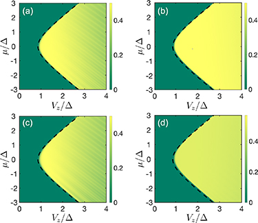
Figure 6. Phase diagram of fermion parity noise of disconnected regions for (a) a 4 m pristine nanowire, (b) an 8
 m pristine nanowire, (c) a 4
 m disordered nanowire and (d) an 8
 m disordered nanowire. The fermion parity noise of disconnected regions faithfully detects topological phase transitions for a good range of and µ.
Download figure:
Standard image High-resolution imageRecent experimental progress in the measurement of fermion parity of SC-SM heterostructures includes various techniques. Circuit-QED based methods [41, 42] involve coupling the desired system to a superconducting resonator and then a fermion parity readout is enabled through the microwave spectroscopy of transitions between the even and odd parity states. An alternative method is parity to charge conversion [40] where the system is tuned such that the parity of the sub-gap states correspond to the charge occupancy of a tunnel-coupled quantum dot. The parity of the system is thus converted to charge of the quantum dot and a measurement of the quantum dot's charge state then provides an indirect parity measurement. The challenge that lies in realizing fermion parity noise as a robust metric for MZM detection is the precise measurement of fermion parity itself. For once the parity is measured accurately, the fermion parity noise is just the statistical variance of the parity measurements. The aforementioned experimental methods can be conveniently integrated into nanowire device setups and facilitate fast electrical readout of the parity, thus helping mitigate the challenge of accurate fermion parity noise measurement.
Lastly, we find it worthwhile to demonstrate the superiority of entanglement entropy (and hence observables such as the fermion parity noise) over techniques with current experimental attention, such as local and non-local differential conductance. In figure 7, we depict the local conductance (GLL
), non-local conductance (GLR
), and the DEE (SD
) of a three-terminal N-TS-N setup involving an intermediate length  m nanowire with minimal to modest disorder. Even under low disorder, the local conductance fails to detect the phase transition with a premature closure, as shown in figure 7(a). The non-local conductance signatures, on the other hand, become obscure and faint under experimentally relevant measurement precision, unable to pinpoint the critical field as depicted in figure 7(b). The DEE, however, remains faithful and accurately signals the phase transition, as shown in figure 7(c).
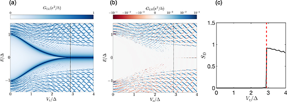
Figure 7. Conductance spectroscopy and the DEE. A comparison of (a) the local conductance, (b) the non-local conductance and (c) DEE of an  m intermediate length nanowire. The chemical potential is kept at 3.2Δ and maximum value of disorder is kept at Δ. Even under a relatively minimal value of disorder, the local conductance closes before the critical Zeeman field (black dashed line in (a)). The non-local conductance becomes faint and signature becomes obscure. Nonetheless, the DEE remains faithful—signaling the transition with pinpoint accuracy.
Download figure:
Standard image High-resolution image4. Conclusion
We proposed and analyzed in depth the use of entanglement entropy and its close relation with topological order for a fool-proof signaling of MZMs in Rashba nanowires. We showed that although the BEE is incapable of determining topological phase transitions, owing to volume and area contributions, the DEE reliably pinpoints topological phase transitions following the distillation of the size contributions. The DEE signatures stay robust to system size and controllable parameters such as chemical potential and magnetic field, even in the presence of disorders such as smooth inhomogeneous potentials at the ends of the nanowire relevant to experimental setups. We explained the quantization of the entanglement entropy in a bottom-up fashion by deconstructing Rashba nanowires as interacting Kitaev Chains. Further, we connected the entanglement entropy signatures to a conserved observable of the system, the fermion parity noise, and illustrated that it displays signatures similar to the entanglement entropy. With active advancement in parity measurement of SC-SM heterostructure, the fermion parity noise emerges as a novel metric for MZM detection. Finally, we concluded by elucidating a simple case with minimal disorder and moderate nanowire lengths where the local conductance signature closes prematurely, and the non-local conductance signature is obscure, but the DEE signature is conclusive and faithfully signals the topological transition. The theoretical methods developed here are of significant relevance toward making experimental progress for the conclusive detection of MZMs, and looking beyond conductance spectroscopy measurements.
Acknowledgments
The authors acknowledge the Visvesvaraya PhD Scheme of the Ministry of Electronics and Information Technology (MEITY), Government of India, as implemented by Digital India Corporation (formerly Media Lab Asia). This work is also supported by the Science and Engineering Research Board (SERB), Government of India, Grant No. MTR/2021/000388 under the MATRICS scheme, the Ministry of Human Resource Development (MHRD), Government of India, Grant No. STARS/APR2019/NS/226/FS under the STARS scheme.
Data availability statement
All data that support the findings of this study are included within the article (and any supplementary files).
Appendix A: Tight-binding Hamiltonian
The Rashba nanowire Hamiltonian is given by

where  is a Nambu spinor and the H is the Hamiltonian density given by

where σi
are the Pauli matrices in the spin basis, and τi
are the Nambu matrices in the particle-hole basis. For our simulation purposes, we discretize this continuous Hamiltonian through the method of finite differences, under which  is replaced by
  , where
  is the discretized annihilation operator and a is the lattice constant. Under this transformation, the Hamiltonian becomes:

where,  and
and 
Appendix B: Entanglement entropy
The entanglement entropy is a measure of entanglement in the system that is derived from the von Neumann entropy. Consider that the concerned quantum system is defined by a Hilbert Space  , the central problem in computing any entanglement entropy of the system (whether bipartite or disconnected) can be mapped to calculating the von Neumann entropy of a partition of the system
  . If the reduced density matrix associated with the subsystem Hilbert space
  is ρA
, then the von Neumann entropy of the subsystem A is given by
is ρA
, then the von Neumann entropy of the subsystem A is given by

where αk
represents the kth eigenvalue of the reduced density matrix ρA
. The steps to calculate entanglement entropy involve first, the calculation of the ground state  of the full system
  , the calculation of the complete density matrix
  of the full system, taking partial trace of the full density matrix to obtain the reduced density matrix
  and then finally diagonalizing ρA
to obtain αk
.
and then finally diagonalizing ρA
to obtain αk
.
The aforementioned procedure is quite computationally tedious. Therefore, we employ the free fermion method of calculating entanglement entropy. If the Hamiltonian of the system is free fermionic in nature, i.e. it contains no bi-quadratic interactions, then we can use Wick's theorem to express the reduced density matrix as

where  and
and  is the effective Hamiltonian for the sub-system A, often known as the entanglement Hamiltonian of the sub-system, which has the same general form as the original Hamiltonian
  , i.e. if the complete system Hamiltonian has N sites and is given in the Nambu space by:
where  . then the subsystem A with M sites has an effective Hamiltonian
  of a similar form
where  .
.
 can now be diagonalized by defining
  with
with  such that
  . Here, ɛ are the eigenvalues and
  is the eigenvector matrix of
  . In this new basis the diagonalized Hamiltonian can be expressed as:

where  .Once the eigenvalues of
  and therefore
  are known, it is straightforward to calculate the eigenvalues of ρA
from (B2) and get the entanglement entropy from (B1).
are known, it is straightforward to calculate the eigenvalues of ρA
from (B2) and get the entanglement entropy from (B1).
However, the issue is that the matrix elements of  are not known. This is where we leverage the idea of correlation matrix. As we will see, the eigenvalues of the truncated correlation matrix are related to the eigenvalues of subsystem Hamiltonian matrix
  and hence
  . But first, we define the correlation matrix and the truncated correlation matrix and how they are computed.
The correlation matrix for the entire system with N sites is defined as:

The expectation values are calculated in the ground-state of the Hamiltonian. The elements of the correlation matrix have the form  ,
,  represents sites and
  represent spins,
  is the ground state of the Hamiltonian.
To evaluate these expectation values, we must first calculate the ground-state of the complete system Hamiltonian. Following from our previous technique, we can diagonalize this Hamiltonian matrix with  , such that
  . The ground state is then constructed with the new BdG operators a as
where  is the fermionic vaccum state.
We then use  to compute the expectation values
Similarly we can get the other terms:

and
The above relations give us the entire correlation matrix C. The truncated correlation matrix  for a sub-system A with M sites is a sub-matrix of the net correlation matrix C which is defined as follows:

Now that we have defined the truncated correlation matrix, we return to our original task of deriving a relation between the eigenvalues of the entanglement Hamiltonian matrix  and the eigenvalues of the truncated correlation matrix. We start by substituting (B2) in (B11) to get:

Substituting (B5) in (B12) gives:
This can be simplified as:
where  . The value of K can be evaluated by imposing the condition
 ![$Tr[\rho_A] = 1$](https://content.cld.iop.org/journals/1367-2630/26/2/023038/revision2/njpad23a2ieqn159.gif) , which is a fundamental property of density matrices. We can now uncover the following:
, which is a fundamental property of density matrices. We can now uncover the following:
Using the above two relations we get:
We can expand  in terms of its eigenvector matrix
  and eigenvalues ɛk
as
and eigenvalues ɛk
as
where  . Thus in terms of λk
,
. Thus in terms of λk
,
It is clear that  and
and  have the same set of eigenvectors and their eigenvalues λk
and ɛk
are related as:
have the same set of eigenvectors and their eigenvalues λk
and ɛk
are related as:

These relations finally lead us to the equation for entanglement entropy in terms of the eigenvalues of the truncated correlation matrix ɛk :
Appendix C: The Keldysh NEGF approach
C.1. Current calculations
First, we start with the assumption that the leads are large enough so that they can be considered semi-infinite, and thus be effectively modeled by infinite dimensional matrices. This assumption allows using the NEGF approach [51] by partitioning the channel and the leads and working with the channel Green's function and incorporating the leads via self energies figure 8. The retarded channel Green's function can now be written as:

where E is the free variable energy, and I is the identity matrix of the dimension of the Hamiltonian, η is a small positive damping parameter, and  and
and  represent the retarded self energies for the semi-infinite contacts.
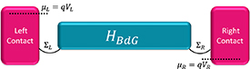
Figure 8. NEGF.
Download figure:
Standard image High-resolution imageThe self energies can be represented in two possible choice of basis: (i) in the eigenbasis of the real-space Hamiltonian, (ii) the eigen basis with wide-band approximation, where the self energy is encapsulated via a parameter  . The contact Hamiltonian can be written in its own eigenbasis as:

where  represents the creation/annihilation operator of the contact momentum eigenstate of spin
  with eigenvalue
  .
.
The coupling between the contacts and the nanowire is given by the tunneling Hamiltonian:

where  represents the annihilation/creation operator of the mth
site of the Kitaev chain and
represents the annihilation/creation operator of the mth
site of the Kitaev chain and  is an element of the tunnel coupling matrix between the
  contact's momentum state k and the mth
site of the Kitaev chain.
contact's momentum state k and the mth
site of the Kitaev chain.
In the basis of the real-space Hamiltonian, the self-energy matrices can be evaluated by a straightforward calculation of the matrix elements  :
:
where P stands for the Cauchy principal value. Recasting this integral into a real and an imaginary part ( ) provides a better physical picture , with the imaginary part
  representing the level broadening, and the real part
  α
calculated from the principal value integral.
α
calculated from the principal value integral.
In this work, we stick to the wide-band approximation basis. Under this approximation,  is independent of energy and thus the principal value integral representing the real-part of the self energy vanishes and we are just left with the broadening matrix
  such that the self energies can be represented as
  , which can be treated as an input parameter. Once we are done calculating the self energies, we need to evaluate the 'lesser' Green's function [51, 52]:

where Ga
is the advanced Green's function (Hermitian conjugate of the retarded Green's function calculated from (C1)). Calculating the lesser Green's function is equivalent to calculating the electron (hole) correlation function. Here,  represent the in-scattering functions from leads L and R respectively which can be evaluated using:

where  represents the Fermi–Dirac distribution in either leads
  with a chemical potential µα
. In this formulation, all different components of the currents can then be deduced from the current operator formula. The elements of the current operator matrix can be deduced using the correlation function and the hopping elements of the Hamiltonian. A rigorous but straightforward calculation based on fundamental consideration gives the current operator matrix:
with a chemical potential µα
. In this formulation, all different components of the currents can then be deduced from the current operator formula. The elements of the current operator matrix can be deduced using the correlation function and the hopping elements of the Hamiltonian. A rigorous but straightforward calculation based on fundamental consideration gives the current operator matrix:

Taking the trace of the above equation gives the net charge current, which is given by the current formula:

The above formula can be further simplified by the notation introduced in with the spectral function  and the electron correlation matrix
  as
as

Using simple manipulations as given below we get:
where  . Using the above in conjunction with (C5) and (C6), along with the properties of the trace operation, yields the Landauer transmission formula for the current as

where  represents the Fermi–Dirac distribution in either lead.
However, in the case involving superconductors, either functioning as a contact or as the central system or both, the net current through the contact α is the difference between electron and hole currents in Nambu space. We can now use the full fledged current operator in (C7) to evaluate the current from first principles as

where  , where is the Pauli-z matrix and is the identity matrix of dimension N × N. The next step is to take a trace of the above equation, which in general need not take the form of (C8), typically when the contacts are superconducting due to the non-diagonal structure of
  , and may lead to erroneous results, specifically when evaluating the Josephson currents. However, in our case, as the contacts are normal, and hence diagonal, (C12) indeed takes the form of (C8) with the net current becoming
where each current  can be evaluated separately using the form in (C8) or (C9). The factor of a half comes since the original Hamiltonian been doubled while writing the BdG Hamiltonian in order to write it consistently in the Nambu space. It is then instructive in our context to note that various matrices defined within the approach will have a matrix structure due to the electron–hole Nambu space. In particular, the contact broadening matrices etc can be written with a general diagonal structure (due to the diagonal structure of normal contacts in Nambu space) as
  , where the superscripts ee(hh) represent the electron (hole) diagonal part of the self energy or broadening matrix (remember that the electron (hole) diagonal part of any matrix only separates sectors in the Nambu space and not the spin space, and therefore both the parts contain both spin types). Following this and using the above observations on the current operator formula in (C9), we obtain the electron (hole) current across the TS as a sum of three components [47, 53]:
and
where the term (i) represents the direct transmission process of either the electron or the hole, (ii) represents the direct Andreev transmission and (iii) represents the crossed Andreev transmission. At this point it is worth noting that  ,
,  . The matrix structure of the broadening matrix Γ itself is diagonal such that
  ,
,  ,
,  ,
,  and zeros otherwise. The Andreev transmission can then be written as
  and the crossed Andreev transmission as
  the direct transmission can be written as
  . Here
  represents the i, j element of the electron (hole) diagonal block of the retarded Green's function in Nambu space and
  represents that of the off-diagonal block of the retarded Green's function in Nambu space.
C.2. Local and non-local conductances
We start with the current formula for a generic bias situation, (VL
,VR
) for the left and right contacts with  and
and 
The current through one of the contacts has contributions from both electron and hole flow. The net current is given by:

The individual electron and hole components can then be derived using:
Here,  and
and  can be shown to be equal and opposite using symmetry conditions and especially:

It is thus sufficient to consider either one of  and
and  while calculating the net current through a contact. Let us now consider the conductance matrix:
Now let us consider only the electron current for now since  . Using this fact we can evaluate the Local conductance as:
At zero temperature, the  where Θ is the Heaviside step function. This implies
  and similarly we can write the other terms. Since the derivative of the heaviside function is the Dirac Delta function, we get:

Now we can similarly get the non local conductance.
Once again, using the property of Fermi–Dirac functions as  as
as  we get:

Appendix D: Spinfull Kitaev Chain
In order to explain the entanglement entropy signatures for the Rashba nanowire from a much more elementary and first-principles perspective, we highlight the parallels between the Rashba nanowire and a toy model consisting two distinct p-wave superconductors interacting through an s-wave pairing potential. Starting with the normal part of the Rashba nanowire Hamiltonian, without proximity-induced superconductivity, in the continuous momentum space:

where,  is the Rashba spin–orbit coupling strength,
  is the Zeeman field, k is the momentum and
  is the fermionic spinor at k. The eigenvalues
  of this Hamiltonian are given by
  . The eigen-spinors in terms of the original spinor are given by:
The spinor basis, defined by  is often called the helical basis. Now we express the full Hamiltonian of the nanowire, including the proximity-induced superconducting pairing terms, in the helical basis. The Hamiltonian in the helical basis [54] is given by:
where,
The Hamiltonian in (3) can be interpreted as follows: there are two bands + and − with their normal parts being described by  and
and  respectively. Within each band, there exists an intra-band superconducting pairing given by
  . These pairings are an odd function of k and hence manifest as intra-band p-wave pairings. There also exists an inter-band superconducting pairing between the two bands given by
  . This pairing is an even function of k and manifests as an inter-band s-wave pairing. Thus, the helical basis allows us to decompose the nanowire into two p-wave superconductors + and − interacting via an s-wave coupling. We notice two things here. First, the effective onsite potential
  depends on a controllable parameter Vz
and therefore the magnetic field B. It decreases with B for the + chain while increases with B for the − chain. Second, the p-wave pairings
depends on a controllable parameter Vz
and therefore the magnetic field B. It decreases with B for the + chain while increases with B for the − chain. Second, the p-wave pairings  are of opposite parity for both bands.
This motivates introducing a new pedagogical model, which we call the 'spinfull Kitaev chain' based on a topical p-wave superconductor—The Kitaev chain. We consider two distinct Kitaev chains, labeled with + and −, interacting via an s-wave pairing potential  . The chemical potentials, hopping terms, and p-wave pairings are represented by µσ
, tσ
,
. The chemical potentials, hopping terms, and p-wave pairings are represented by µσ
, tσ
,  , where
  . The Hamiltonian, describing this pedagogical model, in the position space (with open boundary conditions) is given by:
where  creates a fermion at site 'i' in the
  chain. For further analysis of the model, we express our Hamiltonian in the Majorana basis defined by:
where i represents the site index,  and
and  , where A and B represent two distinct types of Majoranas that constitute a single fermion. In the Majorana basis, our model comprises four interacting Majorana chains. The Hamiltonian in this basis is given by:
In figure 9, we show the decomposition of the spinfull Kitaev chain into four Majorana chains and show the various pairings of Majoranas caused by different terms of the Hamiltonian as solid bonds. In all the figures, the blue spheres with + represent  , the pink spheres with + represent
  , the blue spheres with − represent
  , the pink spheres with − represent
  . The green bonds in figure 9(a) represent the terms
  and
and  , the orange bonds in figure 9(b) represent the terms
  and
and  , the violet bonds in figure 9(c) represent the terms
  and
and  , the black bonds in figure 9(d) represent the term
  .
.

Figure 9. Decomposition of the spinfull Kitaev chain into four interacting Majorana chains. The blue and pink spheres represent A type and B type Majoranas respectively of the ± chains. (a) the green bonds represent couplings due to  and
and  , (b) the orange bonds represent couplings due to
  and
and  , (c) the violet bonds represent couplings due to
  and
and  and (d) the black bonds represent couplings due to
  .
.
Download figure:
Standard image High-resolution imageNext, we study the spinfull Kitaev chain by setting  ,
,  ,
,  ,
,  and we keep
  as the varying parameter. The motivation of varying
  comes from the nanowire model where the + band's effective potential is varied through B. Similarly, we set
  to maintain the opposite parity of the p-wave couplings, just as in the nanowire case. The reason for keeping
  shall be made clear soon. At
  both chains are in the topological regime and have two unpaired Majoranas at their ends. However, due to the presence of an s-wave inter-chain coupling
  , the Majoranas at each end pair up to form a normal fermion, rendering the spinfull Kitaev chain into a trivial phase. This can be seen in figure 10(a), where the yellow unpaired Majoranas hybridize through the solid black bonds caused by
  .
.

Figure 10. Three different cases considered for the spinfull Kitaev chain. (a) The initial case with  . In this case the unpaired Majoranas at the end of both the chains (yellow spheres) hybridise through the inter-chain swave bonding (black bonds). (b) The intermediate case with
  , the intra-chain pairing (green bonds) between Majoranas of the + chain (top chain) has been seeded. (c) The final case with
  . The bonds due to
  dominate the + chain making it trivial and isolating it from any other intra-chain or inter-chain bonds. The bottom chain, however, remains topological with unpaired Majoranas at the ends. Overall the system has two MZMs at the ends.
Download figure:
Standard image High-resolution imageFigure 10(b) represents an intermediate stage where  is finite and can be seen as the green bonds in the top two chains. Figure 10(c) depicts the
  case. Here,
  acts as the only dominating bond in the + chain and decouples the chain + chain from the − chain. The + chain goes into a trivial regime while the − chain stays in the topological regime, allowing there to be effectively two Majoranas at the ends of the wire. This is what precisely happens in the nanowire system, where the effective onsite potential being controlled by the magnetic field B of one band tunes it towards the topological regimes while tunes the other band towards the trivial regime. Before the transition, there are two p-wave superconductors hosting Majoranas. However, their interaction effectively leads to none at the edges. At the topological transition, one band becomes trivial, leading to two unpaired Majoranas at the ends.
Figure 11 shows the entanglement entropy plots for the spinfull Kitaev chain under the settings described above. Figure 10(a) shows the BEE plot for a 100-site chain while figure 11(b) shows the DEE plot for the same chain. Comparing figures 3(a) and 11(a) we see very similar features for both the spinfull Kitaev chain and the nanowire with no quantization and negligible change in the entanglement entropy value over the phase transition. Similarly, comparing figures 3(b) and 11(b) we see that the DEE is zero in the trivial regime and quantized to  in the topological regime in both the spinfull Kitaev chain and the nanowire. A DEE value of
  in the topological regime is logically expected in the spinfull Kitaev chain since chains are now independent of any inter-chain interaction, the + Kitaev chain, being in its trivial regime, contributes 0 units to the DEE while the − Kitaev chain, being topological, contributes
  units [31] to the DEE.

Figure 11. Distillation of the size effects in the spinfull Kitaev model. (a) The BEE (in units of  ) and (b) the DEE (in units of
  ) of a 100 site spinfull Kitaev chain plotted against the chemical potential of the + chain
  . The spinfull Kitaev chain, a pedagogical model of the nanowire system, develops similar entropy signatures to the nanowire system explaining the characteristics of the BEE and DEE plots of the nanowire.
Download figure:
Standard image High-resolution image