


Abstract
The behavior of correlations across a bipartition is an indispensable tool in diagnosing quantum phases of matter. Here we present a spin chain with position-dependent XX couplings and magnetic fields, that can reproduce arbitrary structure of free fermion correlations across a bipartition. In particular, by choosing appropriately the strength of the magnetic fields we can obtain any single particle energies of the entanglement spectrum with high fidelity. The resulting ground state can be elegantly formulated in terms of q-deformed singlets. To demonstrate the versatility of our method we consider certain examples, such as a system with homogeneous correlations and a system with correlations that follow a prime number decomposition. Hence, our entanglement simulator can be easily employed for the generation of arbitrary entanglement spectra with possible applications in quantum technologies and condensed matter physics.
Export citation and abstract BibTeX RIS

Original content from this work may be used under the terms of the Creative Commons Attribution 4.0 license. Any further distribution of this work must maintain attribution to the author(s) and the title of the work, journal citation and DOI.
1. Introduction
Entanglement lies at the heart of the disparity between classical and quantum mechanics. As such it has long been at the forefront of both theoretical [1, 2] and experimental [3, 4] investigations into the foundations of quantum mechanics. More recently, entanglement has gained renewed interest with the development of quantum information theory [5, 6]. In this framework, quantum entanglement is viewed as a valuable resource [7], with several quantum protocols, such as teleportation [8], able to be realized exclusively with the use of entangled states. This new focus has stimulated intensive research into how specific patterns of entanglement can be created and manipulated in quantum many-body systems [9].
One such controllable entanglement property is the scaling of the entanglement entropy, SA , within a bipartite system. The ground states of local quantum lattice Hamiltonians typically obey an 'area law' such that the entanglement entropy is proportional to the size of the boundary of the chosen subsystem, A [10, 11]. In 2010, Vitagliano, Riera and Latorre showed how tuning the coupling profile of the inhomogeneous XX model allows its ground state to transition smoothly from obeying an area law of entanglement entropy scaling to a volume law [12]. The ground state of this model is termed the 'concentric singlet phase' [12] or simply 'rainbow state' [13], due to its distinctive structure of maximally entangled valence bonds connecting pairs of sites distributed symmetrically across the center of the chain. This simple model hosts a rich variety of properties [14, 15] and has been the subject of much interest in recent years [16–19].
In this work we present a generalization of the rainbow state model, whereby, with the introduction of staggered transverse field terms to the inhomogeneous XX model, the degree of entanglement between each concentric pair on the chain can be independently varied. Using a Real-Space Renormalization Group approach we derive recursive expressions for the induced effective coupling and transverse field terms. These expressions have an elegant description in terms of the formalism of q-deformed algebra [20, 21]. For a chain of 2N sites the ground state is a tensor product of N concentric q-deformed singlets, each with an associated deformation parameter, qi
, dependent on the transverse field and coupling parameters of our model. The variation of these physical parameters allows for the generation of any arbitrary set of single-particle entanglement energies. To verify the validity of our results we perform a detailed numerical analysis. This analysis reveals that appropriate choices of the values of the transverse field parameter, and ordering of the degree of entanglement ensures a high fidelity between the exact ground state and the q-deformed rainbow. Moreover, we consider two special cases to demonstrate the applicability of our method. First, we consider the homogeneous case  such that each concentric pair has the same degree of entanglement, mirroring the concentric singlet state of the rainbow chain but generalized to arbitrary degrees of entanglement. Second, we explore a scenario where the entanglement energies of individual particles follow what we refer to as the 'prime number spectrum,' or more precisely, are given by the logarithm of the prime numbers. Under this particular choice, the eigenvalues of the density matrix become the so-called square-free integers, which are integers whose prime factorization solely comprises individual prime numbers without any higher powers. This insight also draws a parallel with the dissection of entanglement spectra in free systems into their constituent single-particle energy components. Such an observation offers a fresh perspective on the logarithm of prime numbers, associating it with the interpretation as the energy states of a fermionic 'primon gas' [22, 23] or as the characteristic periods of closed trajectories within a chaotic quantum system, possibly linked to the Riemann hypothesis [24]. This novel realization holds the potential to shed new light on the intricate interplay between the realms of physics and number theory.
While our quantum simulator gives rise to effective couplings between sites on opposite ends of our chain, our model is completely local, given in terms of XX interactions and local magnetic fields. Thus, it directly lends itself to experimental verification and practical applications. Indeed, recent developments in cold atom experiments [25–30] have offered unique opportunities to simulate such systems and access quantities related to entanglement [31–36]. We expect that our quantum simulator can have direct applications in condensed matter or quantum technologies where specific structures of correlation patterns are requested between two subsystems.
2. The q-deformed model
In order to introduce our model for a chain of 2N spin- particles, we first present a two-site Hamiltonian that allows for direct continuous variation of the degree of entanglement between its spins.
2.1. Two-spin hamiltonian
Consider the two-spin Hamiltonian

The ground state of  is given by
and has ground state energy

where

and ![$[x]_{q}$](https://content.cld.iop.org/journals/1367-2630/26/1/013055/revision2/njpad19f7ieqn4.gif) is the so-called quantum dimension
is the so-called quantum dimension

This ground state is the singlet of the quantum group  [37]. Such q-deformed valence bonds have been considered in relation to a range of many-body models [38–41], including the anisotropic q-deformed generalization of the spin-1 AKLT chain as considered in [42, 43]. In the limit
  such that
  , we recover the maximally entangled singlet state of the standard SU(2) Lie algebra. The degree of entanglement between this pair is directly related to the value of the deformation parameter, q1, which is in turn directly related to our coupling and transverse field parameters via equation (4). To investigate this, we bipartition the system down the center of the chain into region A, and its complement B. The reduced density matrix of (2) is then determined for region A. The corresponding Rényi entropy of order α is given by

and takes the maximum value  when
when  for all α as shown in figure 1. This expression for the Rényi entropy reflects a symmetry of our model as under the transformation
  , such that
  , the value of the Rényi entropy of order α is unchanged.

Figure 1. The variation of the Rényi entropy,  for states given in (2) as a function of their deformation parameter q1, for a range of fixed values of α. The Rényi entropy takes maximal value
  when the deformation parameter
  for all α. This figure is unchanged under the transformation,
  , such that
  , reflecting a symmetry of the Hamiltonian (1).
Download figure:
Standard image High-resolution imageBy considering the limit of  as
as  we obtain the expression for the von Neumann entanglement entropy of the pair

This entropy can be varied continuously to achieve all values in the maximal range  , by varying
  , or equivalently
  . We see that by varying the physical parameters of our model we can achieve all degrees of pairwise entanglement between the two spins.
2.2. 2N-spin hamiltonian
The simple two-spin Hamiltonian presented above is the basis on which we construct our general model for a chain of any even number of spins. We now consider a chain of 2N spin- particles with the following Hamiltonian

We have introduced the site labeling  such that sites −i and i are equidistant from a central bipartition of the chain, as shown in figure 2.
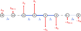
Figure 2. The q-deformed spin model for a chain of 2N sites. The blue lines represent the XX coupling terms, Ji , and the red arrows represent the magnitude and direction of the transverse magnetic field, hi . The magnitude of both the coupling and transverse field are symmetric about the center of the chain, with decreasing strength moving outwards.
Download figure:
Standard image High-resolution imageIn order to find the ground state of our model we have used the Real-Space Renormalization Group approach as first introduced by Ma and Dasgupta in [44] and later developed by Fisher with the application of the method to the Random Transverse Field Ising Chain [45]. This approach allows us to consider the ground state properties of random quantum chains by iteratively decimating the degrees of freedom with highest energy in order to derive an overall effective low-energy model. We start by first briefly reviewing this method with reference to the known results of the  limit of our model.
2.2.1. XX model Renormalization Group
In the limit,  , our Hamiltonian (8) is equivalent to that of the inhomogeneous XX model acting on a chain of 2N spins
where we have re-adopted the standard site labeling  . Using the Renormalization Group (RG) approach for some random coupling profile, the highest energy term such that
  , is identified and diagonalised independently of the rest of the chain. To zeroth-order in perturbation theory, the ground state of the system is then

where  is the maximally entangled singlet ground state of the two-site XX model and
  ,
,  refer to the state of the spins to the left and right of the singlet respectively. To compute higher order corrections to the ground state of our system we consider the spins i and i + 1 to be 'frozen' into this singlet state. Then we employ perturbation theory to find the effect induced by quantum fluctuations on the neighboring spins, as shown in [12]. It is found that an effective coupling arises between sites i − 1 and i + 2 of strength

In this way the coupling between sites i and i + 1 is replaced by effective longer range interaction that captures the low-energy properties of the model. For a random coupling profile, successive iterations of this procedure yield a 'random singlet phase', as singlets form between the pairs of spins most strongly coupled after each decimation. In [12] Vitagliano, Riera and Latorre demonstrated how a coupling profile that decays exponentially away from the center of the chain produces a special form of ground state known as the 'concentric singlet phase'. This ground state is also known as the 'rainbow state', due to it is distinctive structure of a series of singlets symmetrically distributed around the center of the chain. For any given bipartition, the entanglement entropy is directly proportional to the number of singlets 'cut' by the bipartition. Thus, for such a coupling profile, the area law of entanglement entropy is maximally violated.
2.2.2. Q-deformed model Renormalization Group
We now apply the Real-Space RG approach to the generalized model defined in (8). In the limit  , this yields the ground state

to zeroth-order in perturbation theory, where  is the q1-deformed singlet as defined in equation (4). To compute corrections to the ground state at higher orders, second-order perturbation theory is used, as illustrated in figure 3(see also appendix
and transverse field terms

In the case that  this effective Hamiltonian can be diagonalised to yield an additional q2-deformed singlet,
  , between sites −2 and 2, where
  .
.

Figure 3. The Real-Space RG procedure. (a) Our model (8) acting on a chain of four spins. For  perturbation theory yields a q-deformed singlet (4) between the central two spins. (b) These spins are integrated out and an effective Hamiltonian of the form (1) is found to act between sites −2 and 2 with renormalized coupling
  and transverse field
  . (c) Diagonalization of this effective Hamiltonian yields the ground state
  . The difference in color of the bonds between the two pairs indicates the difference in correlations that can be achieved by appropriately tuning
  and h2.
Download figure:
Standard image High-resolution imageIf the couplings throughout the chain are selected such that  , then repeated iterations of this renormalization process will eventually yield the overall ground state

where
and for i > 1

The renormalized coupling and transverse field parameters for the effective Hamiltonian between spins −i and i are given by the recursive expressions
From equations (18) and (19), we see that the expressions for  and
and  are dependent on all previous
  ,
,  . By fixing all previous i − 1 values, it is always possible to vary the associated physical parameters Ji
and hi
such as to achieve any
. By fixing all previous i − 1 values, it is always possible to vary the associated physical parameters Ji
and hi
such as to achieve any  . In this way, we will show that the deformation of each q-singlet can be individually tuned to achieve any degree of pairwise entanglement between a given pair of spins.
3. Entanglement properties of the q-deformed rainbow
The ground state (15) of our Hamiltonian (8) has a tensor product form. Subsequently, the reduced density matrix across a central bipartition admits the tensor product decomposition

where each ρi is diagonal, given by
This decomposition yields simple expressions for many of the entanglement properties of the q-deformed rainbow, as we will see in the following.
3.1. Rényi and von Neumann entropies
Using the reduced density matrix tensor product decomposition we derive the form of the Rényi entropy of order α of the ground state (15) across a central bipartition

In the limit  we obtain an expression for the von Neumann entropy of the ground state

In section 2.1 we found the von Neumann entropy,  , of a single pair of spins as a function of the deformation parameter q1, as given by (6). By extending this definition to that of the von Neumann entropy of the state
  between spins −i and i

it is clear that the total von Neumann entropy is a sum of the individual von Neumann entropies of each concentric pair of spins on the chain. This is also true for the Rényi entropy, and is a natural consequence of the tensor product form of the reduced density matrix. By independently varying each qi
, we can therefore achieve all degrees of entanglement in the allowed maximal range  .
.
3.2. Entanglement spectrum
The entanglement spectrum was introduced by Li and Haldane [46] as an alternative entanglement measure that aimed to capture a complete representation of the entanglement between two subsystems [47]. The values of the spectrum, Ei , are related to the eigenvalues of the reduced density matrix, λi , via

This exponential relationship means that the dominant quantum correlations depend predominantly on the 'lowest' part of the entanglement spectrum.
The entanglement spectrum reflects many of the physical properties of the system [48–52] and serves as a fingerprint of topological order [53–55]. For any non-interacting model, Wick's theorem shows that the spectrum can be constructed from a set of single-particle entanglement energies as
where E0 is a normalization constant and each  [56].
[56].
For our q-deformed rainbow, we find that
and

Hence, the deformation parameters, qi
, of the q-deformed singlets directly determine the single-particle entanglement energies. As each qi
can take any value in the range  , each εi
can be individually tuned to take any value
, each εi
can be individually tuned to take any value  .
.
By combining (17) and (28) we derive the simple relationship

This in turn yields an expression for the required ratio of the renormalized parameters for a given pair in order to produce a specific desired single-particle entanglement energy
As a result, each single particle energy of the entanglement spectrum can be directly obtained by appropriately tuning a single effective magnetic field. In appendix  and J2 is illustrated. For the shown range, any desired ε2 can be simulated by simply reading off the corresponding value of h2. In this way, by fixing all previous i − 1 single-particle entanglement energies, εi
can be tuned to any desired value by appropriately varying hi
.
and J2 is illustrated. For the shown range, any desired ε2 can be simulated by simply reading off the corresponding value of h2. In this way, by fixing all previous i − 1 single-particle entanglement energies, εi
can be tuned to any desired value by appropriately varying hi
.

Figure 4. The values of h2 required to generate any  for fixed
  ,
,  (
( ). Any desired value of ε2 in this range can be obtained by selecting the corresponding value of h2.
Download figure:
Standard image High-resolution image4. Fidelity optimization
In the previous section we have demonstrated how controlled variation of the parameters of our model in the strong inhomogeneity limit  allows for the generation of any arbitrary pattern of correlations given in terms of the entanglement entropy (23) or the single-particle entanglement energies (30). In this section we present how the parameters of our model can be chosen such that the fidelity is maximized for any desired entanglement profile. In quantum information theory, fidelity is a measure of the 'closeness' of two quantum states,
  and
and  , given by the squared overlap,
  [57]. To optimize the choice of parameters for any desired correlation profile, we start by considering the variation of the fidelity between the exact ground state of our model and the q-deformed rainbow for the case N = 2. These results can then be used to inform the fidelity optimization for larger spin chains.
4.1. Optimising h2
In section 2.1, we noted that a symmetry of our two-site Hamiltonian (1) results in the preservation of the von Neumann entropy,  , under the transformation
  . Here, we will show that although
  possesses a similar symmetry under the transformation
  , one of these values will yield a significantly higher fidelity than the other corresponding to the choice of sign of
  .
.
In figure 5 we plot the fidelity between the q-deformed rainbow and the exact ground state of (8) as a function of the entanglement entropy between sites −2 and 2 for a range of constant values of h1. For each curve  and J2 are fixed such that
  is a function of h2. We see that for any desired value of
  , for example
  as indicated by the vertical gray line, the two intersections with each curve indicate two values of h2 that correspond to the same degree of entanglement, but with a distinct difference in fidelity. As described these two solutions arise due to the natural symmetry of the entanglement entropy about
  , for which the degree of entanglement between sites −2 and 2 is maximized. To find the physical transverse field value
  that maximizes
  we substitute
  into equation (14) to obtain
The symmetry of the entanglement entropy  about
about  is shown in figure 6(a) for the case
  ,
,  . By mapping these values onto the plot of fidelity with
  as shown in figure 6(b), we see that we have a 'high fidelity branch' corresponding to
  (
( ) and a 'low fidelity branch' for
  (
( ). For any desired value of
  , the fidelity is clearly maximized by choosing the appropriate value of
  . In contrast, if the sign of h1 is reversed while J1 remains fixed, as shown in figures 6(c) and (d), the opposite is true, and the fidelity is maximized by selecting the value of h2 from the branch
  . In this way, for fixed couplings J1 and J2, the magnitude and direction of the applied magnetic field terms h1 and h2 can be selected such as to maximize the accuracy of our model.

Figure 5. Variation of the ground state fidelity with the entanglement entropy of the outer pair for different fixed values of h1 with  and
and  . The gray line shows an example of a desired outer entanglement entropy,
  . The two intersections with each curve for
  indicate two possible values of h2 to generate the desired
  with a distinct difference in fidelity. This choice can be used to optimize the accuracy of our model.
Download figure:
Standard image High-resolution image
Figure 6. (a) Variation of the entanglement entropy of the outer pair with h2 for  and
and  . (b) The corresponding variation of the ground state fidelity with the entanglement entropy for both the values less than and greater than
  . The higher fidelity branch corresponds to the values
  . (c) Variation of the entanglement entropy of the outer pair with h2, now for
  ,
,  and
and  . (d) The corresponding variation of the ground state fidelity with the entanglement entropy for both the values less than and greater than
  . The higher fidelity branch now corresponds to the values
  . On all four subfigures the solid gray line serves to illustrate this fidelity optimization for the specific case
  .
.
Download figure:
Standard image High-resolution image4.2. Optimizing order of pairs
Our system has a symmetry with respect to which pair of spins i and −i is used to tune a certain single particle entanglement energy εk . We can use this freedom, in conjunction with the optimization procedure of the previous subsection, to optimize the overall fidelity of our chain simulator.
Consider the case in which we want to use our model to generate a given pair of two-site von Neumann enanglement entropies, for example,  and
and  . Our simulator has the freedom in the choice
  or
or  . In figure 7 we plot the two curves corresponding to
  , and
, and  for
for  ,
,  and h1 tuned accordingly. The analysis of the previous subsection has been applied to restrict to the appropriate high fidelity branch
  . From figure 7 we observe that our model can be used to achieve
  with a significantly higher fidelity than
  . The importance of the ordering of the degrees of entanglement is further illustrated in figure 8 with a direct comparison of the fidelity with the degree of entanglement between one pair when the other is maximally entangled. For all values of
  , it is observed that the fidelity is maximized when the maximally entangled state lies between sites −2 and 2.
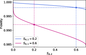
Figure 7. The variation of the fidelity with  for
for  and
and  (
( ,
,  ). Suppose that one wishes to use our simulator to achieve
  between one pair of sites and
  between the other. The dashed lines shown indicate the notably higher value of fidelity that can be achieved by choosing our parameters such that we have the ordering
  .
.
Download figure:
Standard image High-resolution image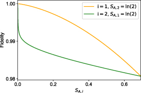
Figure 8. The fidelity of the four-site q-deformed rainbow and the exact ground state of our model when one pair is maximally entangled and the entanglement entropy of the other is varied ( ). For every combination of entanglement entropies, the fidelity is maximized by choosing our parameters such that the maximally entangled pair is between sites −2 and 2.
Download figure:
Standard image High-resolution imageIn appendix  or entropies
  the corresponding field and coupling terms can be substituted into equation (C9) in order to directly determine the ordering that will optimize the fidelity.
4.3. Fidelity analysis for larger chains
In the previous two subsections we have shown that appropriate choices of the values of the transverse field parameters, and ordering of the degree of entanglement allow us to optimize the fidelity and thereby the accuracy of our model for the case N = 2. Although the simplest non-trivial implementation of our model, these techniques derived for the four-spin chain can also be used to optimize the fidelity of our simulator on larger chains. For example, in section 5.2 we will introduce an example of a non-uniform spectrum that our model can simulate known as the 'prime number spectrum', in which the single-particle entanglement energies for a chain with N pairs are the logarithms of the first N prime numbers. Performing a numerical optimization procedure for this spectrum on 10 sites with a coupling profile of the form  we find that the fidelity is maximized when
  . Choosing our coupling and transverse field terms such as to produce the single-particle energies in this order ensures that the ground state of (8) matches our q-deformed ground state with a fidelity
  . To highlight the importance of this choice we note that in contrast, using our simulator to produce the same spectrum with alternate ordering
  , yields a fidelity of only 0.878 to three decimal places.
Thus, our analysis for the case N = 2 also aids in the application of our simulator to larger chains. For larger chains however, there are additional features that we must discuss. We start by noting that, although our model is theoretically exact up to the thermodynamic limit, in practice, the balance between the rapid decay of our coupling and transverse field parameters ensuring the validity of our real-space RG approach and the finite precision of computational methods, only allows us to numerically simulate small system sizes. Such restrictions were discussed in the original work on the rainbow state model [12]. To perform error analysis on the system for larger chains we must therefore choose a coupling profile and single-particle entanglement energy spectrum known to yield a high fidelity. Here we will consider the effect of random errors on the simulation of the optimized prime number spectrum on 8 sites,  for the coupling profile
  . This spectrum can be achieved with a fidelity
  . For some fixed Δ we generate a profile of random errors
 ![$\{\delta_{i}\} \in [-\Delta,\Delta ]$](https://content.cld.iop.org/journals/1367-2630/26/1/013055/revision2/njpad19f7ieqn138.gif) , such that our parameters
, such that our parameters  and
and  . For these altered parameters, equations (18), (19), (28) and (30) can be used to find the new entanglement spectrum and q-deformation parameters. These values can then be used to find a modified form of the q-deformed rainbow ground state. By taking the overlap between this state and the q-deformed rainbow for our desired entanglement profile we calculate a value for the fidelity. For each Δ this process is repeated 10 000 times and an average value for the fidelity calculated. The results for a selected range of Δ are shown in figure 9. We observe that as mentioned above, this drop in fidelity with the increasing size in error is related to the size of the weakest parameters in our model. As the size of the couplings and transverse fields increase from left to right we observe a drop in the fidelity each time the size of the error exceeds the magnitude of one of these parameters. Naturally, as our parameters become smaller with an increasing number of sites on our chain, the accuracy of our model becomes increasingly sensitive to errors.
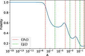
Figure 9. The results of our random error analysis for the optimized prime number spectrum on 8 sites 
 for the coupling profile
  . The value Δ parameterize the size of error introduced into the system such that each desired Ji
and hi
are modified by an amount
. The value Δ parameterize the size of error introduced into the system such that each desired Ji
and hi
are modified by an amount ![$\delta_{i} \in [-\Delta, \Delta]$](https://content.cld.iop.org/journals/1367-2630/26/1/013055/revision2/njpad19f7ieqn129.gif) . The fidelity plotted for each value Δ is the average overlap between the predicted q-deformed ground state and the q-deformed ground state with the modified coupling and transverse field terms for 10 000 randomized
. The fidelity plotted for each value Δ is the average overlap between the predicted q-deformed ground state and the q-deformed ground state with the modified coupling and transverse field terms for 10 000 randomized  profiles. The dashed orange and green lines represent the strength of our coupling and transverse field terms respectively. We see that the fidelity begins to drop as the value of Δ surpasses the weakest parameter in our model. As the size of these terms increase from left to right we observe a drop in the fidelity each time the size of the error exceeds the magnitude of one of these parameters.
Download figure:
Standard image High-resolution image5. Special cases
We have shown how the tuning of the parameters of our model allows for the generation of any arbitrary set of single-particle entanglement energies. In this section we highlight two interesting applications: the case in which all deformation parameters are equal, and the reproduction of the single-particle entanglement energies for the 'prime number spectrum' introduced below.
5.1. The  Case
Case

In the rainbow state model, the ground state is a tensor product of concentric maximally entangled singlets, or in the language of our model,  , for all i. Here, we show how the parameters of our model can be chosen such that all deformation parameters take the same value,
  , for some chosen q in the allowed range
  . In this way, each concentric pair on our chain shares the same degree of pairwise entanglement, and all single-particle entanglement energies are equal.
We have defined  and
and  , such that the condition
  . Re-arranging equation (4) and setting
  yields

for some desired q > 0.
For all other pairs of sites the relations for the normalized couplings must be used. For example, by dividing equation (14) by equation (13) and equating with (32) we obtain
For any fixed value of J2 this relation can be easily implemented to find the required transverse field parameter to produce some desired q > 0.
In the same way, the ratio of equations (18) and (19) can be equated with (32) in order to obtain the general formula
By iterating through and systematically determining each successive value of the required transverse field for some fixed coupling profile, these relations allow us to produce a one-dimensional chain in which each concentric pair shares the same degree of pairwise entanglement.
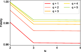
In figure 10 the variation of the fidelity with system size is plotted for a range of values of q. For each fixed number of sites on the chain, the fidelity increases with the value of q, corresponding to a better simulation of chains with a lower degree of entanglement between the pairs. The case with lowest fidelity corresponds to the reproduction of the rainbow state with q = 1 such that  for all i. For each fixed value of q, as the number of sites on the chain increases the fidelity drops off, rapidly for the increase from 2 to 3 pairs, then more slowly up to 5 pairs.
Figure 10. Variation of the fidelity with system size for the special case of homogeneous entanglement. For each value of N on a given curve, the q-deformation parameters that quantify the degree of entanglement between each concentric pair are fixed such that  . For each value of N, the fidelity increases with the value of q, indicating a more accurate simulation of chains with a lower degree of entanglement between the pairs. For each fixed value of q, as the number of sites on the chain increases the fidelity drops but remains high for up to 5 pairs on our chain.
Download figure:
Standard image High-resolution image
5.2. Prime number spectrum
Prime numbers play an important role in number theory. The Fundamental Theorem of Arithmetics [58] states that every natural number greater than one can be uniquely factorized as a product of prime numbers

where p is a prime and np counts the number of times that p appears in the factorization of N. In this way, prime numbers can be thought of as the building blocks of all natural numbers.
Let us introduce the Möbius function,  :
:
where p are prime numbers. The symbol  means that p2 divides n. A square free integer is an integer whose factorization into products of primes does not contain any square of a prime numbers.
  is therefore non-vanishing only on square free integers with value +1 if it contains an even number of primes and −1 if it contains an odd number of primes. In this way, the function µ is a sort of Fermi statistics if one thinks of the primes as being fermions [23].
Let us now consider an entanglement spectrum of the form

The normalization of the eigenvalues implies that

where we have used the Euler product formula

Using equation (25), the entanglement energies for this spectrum are given by

Where k is any square free integer. We equate this expression with that of the spectrum of a free fermionic system
If k is a square free integer then from the Fundamental Theorem of Arithmetics one has

such that taking the logarithm of (42) yields

Hence, equation (41) is solved by


The parameter s can be thought of as an entanglement temperature since it is common to all eigenenergies. The relation (45) has also been considered in [22, 23] with  being the single-particle energies of the primon gas. The partition function of this gas is related to the Riemann zeta function,
  . In recent work, a prime number eigenvalue spectrum has also been experimentally realized by application of holographic optical traps [59], in agreement with previous theoretical results [60].
This example spectrum (45), motivated by the interesting parallel between the decomposition of integers in terms of prime numbers and the decomposition of free-system entanglement spectra in terms of single-particle energies, provides an example of a non-uniform entanglement spectrum that can be reproduced using our q-deformed model. To implement this spectrum for some finite number of pairs with fixed coupling profile  , the required values of the set
  , can simply be read off from equations (B1)–(B3) in appendix
6. Conclusions
In summary, we have introduced a spin chain that can produce arbitrary ground state free-particle correlations across a given bipartition. Our scheme is a generalization of the rainbow states of concentric maximally entangled singlets to the case of concentric pairs, each one with arbitrary entanglement. The degree of entanglement is easily tuned by appropriately choosing the magnitude of local magnetic fields. The entanglement across the bipartition can be parameterized in terms of single particle energies of the entanglement spectra. We find that for a fixed coupling profile these energies are simple functions of the magnetic fields, thus providing direct accessibility and tunability.
To test the validity and applicability of our method we compare the fidelity of the predicted theoretical model with the exact diagonalisation of the spin system. The employed perturbation method has a symmetry in terms of the ordering of the concentric entangled states. By taking advantage of this symmetry we find the optimal order of magnetic fields that gives the best fidelities. Finally, we apply our method to two case scenarios. First, we consider the homogeneous case of concentric pairs with the same entanglement. Second, we consider the case of single particle energies of the entanglement spectra that are parameterized by the logarithms of the prime numbers. This model is inspired by the similarity between the decomposition of free-system entanglement spectra in terms of single particle energies and the decomposition of integers in terms of prime numbers. In recent experimental work, holographic techniques have been developed allowing for the tuning of the energy spectrum of the single-particle Schrödinger equation [59]. Notably a 'prime number quantum potential',  , can be applied such that the single-particle Schrödinger equation has the lowest N prime numbers as eigenvalues. These techniques demonstrate an interesting procedure for the reproduction of arbitrary sequences of integers as energy spectra with possible applicability to this work.
Our methodology can have a direct application in quantum technologies, whenever a very specific pattern of quantum correlations is required [61–63]. It can also simulate quantum phases of matter that require specific ground state correlations across a bipartition. Finally, our approach opens the way to investigate inhomogeneous spin chains in the presence of disordered magnetic fields, which is physically a common scenario, thus generalizing previous approaches [17, 64].
Acknowledgments
We would like to thank Gabriel Matos and Andrew Hallam for inspiring conversations. L B acknowledges support from EPSRC Grant No. EP/T517860/1. This work was also in part supported by EPSRC Grant No. EP/R020612/1. G S acknowledges financial support through the Spanish MINECO grant PID2021-127726NB-I00, the Comunidad de Madrid Grant No. S2018/TCS-4342, the Centro de Excelencia Severo Ochoa Program SEV-2016-0597 and the CSIC Research Platform on Quantum Technologies PTI-001.
Data availability statement
All data that support the findings of this study are included within the article (and any supplementary files).
Appendix A: Four site perturbation theory
In order to illustrate the Real-Space RG approach, we apply perturbation theory to our Hamiltonian (8) restricted to a chain of four sites

where

is our original two-spin model and

Here the couplings  and
and  , such that for any
  , the perturbative condition
  is ensured.
On two sites,  has the following eigenstates


with eigenenergies ![$E_{1} = -[2]_{q_{1}}J_{1}, E_{s} = 0, E_{t} = 0$](https://content.cld.iop.org/journals/1367-2630/26/1/013055/revision2/njpad19f7ieqn164.gif) and
and ![$E_{k} = +[2]_{q_{1}}J_{1}$](https://content.cld.iop.org/journals/1367-2630/26/1/013055/revision2/njpad19f7ieqn165.gif) respectively, and q1 as previously defined in equation (4).
respectively, and q1 as previously defined in equation (4).
When extended to a chain of four spins, the ground state subspace of  becomes four-fold degenerate. We represent this subspace with the basis vectors:
  ,
,  ,
,  . The first-order corrections arise due to the action of the perturbative term on the ground state subspace. This is quantified via the computation of the matrix elements of the effective Hamiltonian to first order

yielding
in the basis  . By inspection, it can be seen that the first-order effective Hamiltonian term is therefore
  . The first-order ground state energy correction is found by diagonalizing the above matrix. It is clear that the degeneracy is only partially lifted to first order. It is therefore necessary to consider the second order corrections that arise due to the overlap with states from each of the excited state subspaces. These excited state subspaces are found in the same way as the set
  by taking the tensor product of the two-qubit computational basis with the excited eigenstates of
  :
:  ,
,  ,
,  ,
,  ,
,  ,
,  ,
,  ,
,  ,
,  ,
,  ,
,  ,
,  . Such that the full set of excited states,
  .
.
The matrix elements of the effective Hamiltonian to second-order are found from

The computation of which yields
Combining our first and second-order perturbative terms we derive an expression for the effective Hamiltonian correct to 

In this way we obtain the following expressions for our renormalized parameters
Note that, in the case  such that
  ,
,  vanishes and
  returns to that of the inhomogeneous XX model re-scaling as seen in equation (11) as expected.
Diagonalization of the effective Hamiltonian yields the ground state
with corresponding ground state energy
where

Appendix B: Relationship between real model parameters and single-particle entanglement energies
In section 3.2 the following relationship was found between the renormalized coupling parameters and single-particle entanglement energies
By combining this relation with equations (18) and (19), we can obtain expressions that directly relate the desired single-particle entanglement energies to the required ratio of real parameters in our model. The recursive nature of the formulae for the re-scaled parameters means that in order to engineer some single-particle energy, εi , it is necessary to have previously established some value for all previous i − 1 energies.
In the strong inhomogeneity case  that we consider, the central terms J1 and h1 do not get re-scaled, therefore simply

for some desired single-particle energy, ε1, and fixed value of the central coupling term. In appendix A we have found exact expressions for the renormalized parameters  and
and  . By substituting these into (30) and fixing all other parameters, we obtain an expression for the required transverse field

Repated iterations of this process yield a general form for the required transverse field parameter for any pair of sites −i and i, when i > 2

Thus, it is made explicit how the real parameters of our model can be selected such as to produce any desired set of single-particle entanglement energies.
Appendix C: Analytic fidelity for N = 2
Here we present an analytic expression for the fidelity between the ground state of the model (8) and our q-deformed rainbow for the case N = 2. The Hamiltonian  is a function of four parameters
  and h2. With a re-ordering of the basis states the associated
  matrix takes on a block diagonal form with the largest
  sub-matrix yielding the unique ground state of the form,

where  is the appropriate normalization factor. Choosing a = 1 the other co-efficients are related to our variable parameters in the following way


where  is the exact ground state energy with
  and
and  .
.
Using equation (15), our q-deformed rainbow ground state on four sites has the form
The ground state fidelity that we use to quantify the accuracy of our method is defined as the squared overlap between the exact and q-deformed ground state

Thus for some desired pair of single-particle energies  , with a choice of coupling profile for J1 and J2,
  and h2 can be found and substituted into (C9) to determine an exact value for the fidelity.