Spectral properties of two coupled Fibonacci chains

Aperiodic structures, in particular quasicrystals [1], have attracted the attention of researchers for many decades [2–6]. Even the simplest quasiperiodic, one-dimensional models exhibit a rich variety of behavior, ranging from critical eigenstate localization properties, to the appearance of energy spectra that sometimes form a fractal set [7]. The tools used to understand these behaviors include, but are not limited to, renormalization procedures, multifractal analysis, or symmetry considerations [8–10]. One of the peculiar features that these systems show is a hierarchical structure of energy gaps [9]. This gives rise to spectral measures that are singular continuous, such as the fractal set observed in the Fibonacci quasicrystal [6]. This is a feature that was linked to all the critical localization properties observed in quasicrystals as well as other systems that possess some type of aperiodic order [7].

Although the behavior of aperiodic chains has been investigated extensively and in great detail, comparatively little work has been dedicated to the case where two or more chains are coupled to each other, forming an aperiodic ladder [11–15]. In this work, we take a step into this realm by analyzing a range of different coupling schemes between two identical one-dimensional Fibonacci chains. Specifically, we study cases where the two chains are directly coupled in a uniform, non-uniform, or quasiperiodic manner, and evaluate the resulting spectral properties, namely the energy eigenvalues and eigenstates. Additionally, we study a special case of an indirect coupling, that is, two chains coupled to each other through some intermediate sites. These cases are easily tractable, since they posses a reflection symmetry which allows to block-diagonalize the Hamiltonian.

We find different spectra depending on the setup. In the case of uniform coupling, the eigenvalue spectrum is identical to that of two uncoupled Fibonacci chains, but with shifted energy eigenvalues. On the other hand, if the two chains are coupled only through a single site, the spectrum consists of two Fibonacci chains with an on-site defect. The structure of the eigenvalue spectrum becomes more complex for the case of quasiperiodic coupling, for which a richer hierarchical structure reveals itself through a perturbative renormalization approach. If only the sites of one specific type (A or B) are coupled to each other, we show that, for a specific value of the interchain coupling, half of the eigenstates are critical, while the other half are extended. Interestingly, these two different classes of eigenstates possess different parity with respect to a corresponding reflection operation and can thus be selectively excited by incoming waves of negative or positive parity. This could be used to control the transport properties of this system. Finally, we also realize couplings between the chains through some intermediate sites. This leads to the appearance of flat bands in a quasiperiodic lattice.

This paper is organized as follows. To be self-contained, we start by briefly reviewing the properties of the Fibonacci chain in section 2, followed by an overview of the methods used to generate our results in section 3. In section 4, we analyze the simplest way of coupling two Fibonacci chains, namely a uniform one. In section 5, we investigate different cases of non-uniform coupling. We start by connecting only sites of a specific type to each other in section 5.1. Then, in section 5.2, we analyze the case where only two sites are coupled. In section 6, we couple the two chains in a quasiperiodic fashion and analyze the resulting eigenvalue spectrum in terms of a renormalization scheme. Finally, in section 7, we consider the scenario where the two chains are not directly coupled to each other, but through intermediate sites. Our conclusions are presented in section 8.

We consider a general Fibonacci chain model, namely a nearest-neighbor tight-binding chain with periodic boundary conditions, so that the chain effectively becomes a ring. The on-site potential and hopping amplitudes are both modulated by the Fibonacci sequence, and the corresponding Hamiltonian is given by

$$\begin{equation} H_{F} = \sum_{i = 1}^{N} v_{i} \vert i\rangle \langle i\vert + \sum_{\langle i,j \rangle}h_i \vert i\rangle \langle \,j\vert \end{equation} \tag{ 1 }$$

where $\vert i\rangle$ denotes a basis state fully localized on the ith site and $\langle i,j \rangle$ denotes nearest-neighbors. The on-site potential v_i and the hopping amplitude h_i are both binary and follow the sequence of a Fibonacci word S_n of generation n. The latter is defined by the recursion relation

$$\begin{equation*} S_n = S_{n-1}S_{n-2}, \ \ n\geqslant 2, \end{equation*}$$

which is a binary representation of the Fibonacci sequence. This inductive recursion formula is expressed as a string concatenation instead of number addition. Another typical representation is through the substitution rule A → AB and B → A. With the initial two words being $S_{0} = B$, $S_{1} = A$, the first few words are thus

$$\begin{align*} S_{0} & = B \\ S_{1} & = A \\ S_{2} & = AB \\ S_{3} & = ABA \\ S_{4} & = ABAAB \\ S_{5} & = ABAABABA \\ S_{6} & = ABAABABAABAAB \, . \end{align*}$$

We note that the Fibonacci sequence is most commonly represented in numeric form through the recursion formula

$$\begin{equation*} F_n = F_{n-1}+F_{n-2}, \ \ n\geqslant 2, \end{equation*}$$

where $F_{0} = F_{1} = 1$ and F_n is the $n\text{th}$ Fibonacci number, which is equal to the word length $|S_n| = F_n$. Another important property of the sequence is that, in the thermodynamic limit, the ratio between the amount of letters A and B is equal to the golden ratio φ. This is more appropriately expressed as [16]

$$\begin{equation*} \lim_{n\to\infty}\frac{F_{n}}{F_{n-1}} = \frac{1+\sqrt{5}}{2}\equiv\phi \, . \end{equation*}$$

The Hamiltonian (1) can be studied in its general form or reduced to a purely on-site or hopping Fibonacci model, where the parameters $h_i = h$ or $v_i = v$ are uniform. These have been termed diagonal and off-diagonal models in the literature, while equation (1) is referred to as the mixed model. All these models have been studied previously in their various forms [17–20], but one important aspect is the equivalence between the on-site and hopping models under a perturbative renormalization scheme [18]. This means that we can uncover all essential features by studying the unmixed models. For this reason, we will focus on the on-site model for our analysis. In this case, the on-site potential v_i of the ith site is equal to either v_A or to v_B , depending on whether the ith character of S_n is equal to A or to B, and the hopping parameter is constant and equal to h. We note that the number of sites in the chain is then equal to $|S_n| = F_n$. Figure 1(a) shows a graphical representation of such a Fibonacci chain. Due to the periodic boundary conditions, the depicted system constitutes the unit cell of a periodic approximant of the quasicrystal (if $N\to\infty$, it becomes a proper quasicrystal). This is a system which has long-range order, without being periodic. Its eigenstates form a set of critical states, which have atypical localization properties. This means that they are neither extended nor localized [7]. The eigenvalues have a spectral measure that is singular continuous and form a fractal set (a Cantor set of measure zero). This feature is also observed in the eigenstates, with wavefunctions that show multifractal properties [10]. In figure 1(b), the eigenstates of a Fibonacci chain with N = 89 are graphically depicted.

Zoom In Zoom Out Reset image size

The properties of quasicrystals have been studied in a multitude of ways, ranging from perturbative methods based on a renormalization formalism [9, 18] to exact results using a transfer matrix approach [21] or a symmetry perspective, which offers insights on the fragmentation of states in terms of local spatial structures of the chain [22].

Before we continue, let us briefly comment on possible realizations of the Hamiltonian equation (1). We note that the following statements also hold for the more complex models that we will present later in this manuscript. Since we treat the matrix eigenvalue problem $H \vert \Psi\rangle = E \vert \Psi\rangle$, the setups proposed in this work are well suited for a realization in various systems modeled by such a problem, as long as the relevant matrix elements that correspond to couplings and on-site potentials of our Hamiltonian can be controlled. An immediate candidate, for instance, are systems of evanescently coupled optical waveguides [23]. Here, each site corresponds to a monomodal waveguide. By suitably tuning quantities such as waveguide shape, spacing, the on-site potentials v_i and couplings $h_{i,j}$ are tunable in a wide range. We remark that the propagation of light in such arrays of evanescently coupled photonic waveguides can be described by a discrete, time-dependent Schrödinger equation, which would also allow to probe the dynamics of the setups proposed in this work. Another realization that is directly feasible is in terms of electric circuits, where the sites are nodes of the circuit, and with on-site potentials and couplings being determined by how the nodes are grounded and interconnected to each other [24, 25].

In this section, we will provide a comprehensive description of the methods employed to calculate and illustrate the relevant quantities before delving into the obtained results. We will begin by explaining the numerical methods utilized in this study, which encompass the creation of all eigenstate maps. Subsequently, we will outline the analytic methods employed to describe the section concerning quasiperiodic coupling.

3.1. Numerical methods

3.2. Analytical methods

3.2.1. Hierarchical splitting and renormalization

The main analytic tool used in this work is a perturbative renormalization procedure based on the degenerate Brillouin–Wigner perturbation theory, described in the works of Niu and Nori [9, 18].

Consider a one-dimensional chain described by a tight-binding Hamiltonian that incorporates a set of hierarchical hoppings, where the hopping strengths follow the relation $T_j\ll T_{j-1}\ll \cdots T_{2}\ll T_1$ (as depicted in the topmost chain of figure 2). In this scenario, we can employ a perturbative renormalization approach to calculate the energy levels of the topmost chain.

Zoom In Zoom Out Reset image size

This perturbative renormalization approach involves treating the weaker hoppings (T_j with higher indices) as perturbations to the dominant hopping term (T₁). This allows us to systematically incorporate the effects of the weaker hoppings and compute the resulting energy levels of the topmost chain. This is done by using the subset of unperturbed degenerate eigenstates as the basis set for the perturbed Hamiltonian. We then apply Brillouin–Wigner perturbation theory to calculate the effective couplings between these states. In figure 2, this process is visually represented by the middle chain, where each blue site represents a (anti)bonding degenerate eigenstate of the T₁ molecule. By considering these (anti)bonding states as the basis, we can determine the effective couplings induced by the weaker hoppings (T_j ) and calculate the resulting energy levels of the topmost chain. In principle, this process is repeated indefinitely, but in practice, one takes a chain of finite size and imposes periodic boundary conditions to perform the calculations. The energy levels form a cluster of 2^j values around the base energy E₀

$$\begin{equation} E = E_0\pm T_1\pm\frac{T_2}{2}\pm\cdots\pm\frac{T_j}{2^{j-1}} \,. \end{equation} \tag{ 2 }$$

3.2.2. Brillouin Wigner perturbation theory

We shall now give a brief overview of Brillouin–Wigner perturbation theory. Consider a Hamiltonian $H = H_0+H_1$, with H₁ acting as a perturbation to H₀. Let E₀ be a degenerate energy eigenvalue, and Q denote the projection operator onto the corresponding degenerate subspace. We also denote the complementary projection operator $P = \unicode{x1D7D9}-Q$. The eigenvalue equation $H\vert \psi\rangle = E\vert \psi\rangle$ can be rewritten such that

$$\begin{equation} P\vert \psi\rangle = P\frac{1}{E-H_0}H_1\vert \psi\rangle = P\frac{1}{E-H_0}PH_1\vert \psi\rangle \end{equation} \tag{ 3 }$$

where the last equality follows from $P^2 = P$ and $PH_0 = H_0P$. We now write

$$\begin{align*} \vert \psi\rangle & = (Q+P)\vert \psi\rangle \\ & = Q\vert \psi\rangle +P\frac{1}{E-H_0}PH_1\vert \psi\rangle \\ & = Q\vert \psi\rangle +P\frac{1}{E-H_0}PH_1(Q+P)\vert \psi\rangle \\ & \,\,\,\,\vdots \\ & = \sum_{n = 0}^\infty\left(P\frac{1}{E-H_0}H_1\right)^nQ\vert \psi\rangle , \end{align*}$$

where we have just consistently used equation (3). With the above equation, we can now easily obtain an effective Hamiltonian for the degenerate subspace with eigenvalue E₀ through a left multiplication by QH,

$$\begin{equation} \begin{split} QH\vert \psi\rangle = EQ\vert \psi\rangle & = \left[QH_0Q+QH_1\sum_{n = 0}^\infty\left(P\frac{1}{E-H_0}H_1\right)^nQ\right]Q\vert \psi\rangle \\ &\equiv H_{\text{eff}}Q\vert \psi\rangle \end{split}. \end{equation} \tag{ 4 }$$

Using this effective Hamiltonian, it will be possible to understand the structure of the spectrum in the case of quasiperiodic coupling, which is treated in section 6.

Let us investigate the setups where two such chains—each consisting of N sites and with periodic boundary conditions—are coupled to each other in different ways. We will focus on the impact of these different coupling schemes on the corresponding spectral properties.

The first and simplest scenario occurs when the two chains are uniformly coupled to each other, as shown in figure 3(a). The setup is then described by

$$\begin{equation} H = H_{I} + h^{^{\prime}} \sum_{i = 1}^{N} \Big(\vert i_{u}\rangle \langle i_{l}\vert + \vert i_{l}\rangle \langle i_{u}\vert \Big) \end{equation} \tag{ 5 }$$

with

$$\begin{equation} H_{I} = \sum_{x = u,l}\sum_{i = 1}^{N} v_{i} \vert i_{x}\rangle \langle i_{x}\vert + h \sum_{x = u,l}\sum_{\langle i,j \rangle} \vert i_{x}\rangle \langle \,j_{x}\vert \end{equation} \tag{ 6 }$$

where $\vert i_{u}\rangle$, $\vert i_{l}\rangle$ denote basis states fully localized on the ith site of the upper or lower chain, respectively. We note that such a setup has been investigated in [26], though with a focus on the density of states and not on the eigenvalues and eigenstates.

To understand the impact of such a uniform coupling, we employ the up/down mirror symmetry of the setup. Due to this symmetry, the eigenstates have definite parity under an exchange of the lower and upper chain. This fact can be used to construct a symmetry-adapted basis $\mathcal{S}$, consisting of N states of positive parity

$$\begin{equation} \vert 1_{u}\rangle + \vert 1_{l}\rangle , \ldots{}, \vert N_{u}\rangle + \vert N_{l}\rangle \end{equation} \tag{ 7 }$$

and N states with negative parity

$$\begin{equation} \vert 1_{u}\rangle - \vert 1_{l}\rangle , \ldots{}, \vert N_{u}\rangle - \vert N_{l}\rangle \, . \end{equation} \tag{ 8 }$$

Written in this basis, $H^{^{\prime}} = \mathcal{S}^{-1} H \mathcal{S}$ consists of two isolated subsystems, $H_{+}$ and $H_{-}$. These two subsystems are shown in figure 3(b). It can be seen that each of them is equal to an isolated Fibonacci chain of N sites, though with on-site potentials uniformly shifted by an amount of plus or minus hʹ. That is, $H_{\pm} = H_{I} \pm h^{^{\prime}} I$, with I being the identity matrix.

Let us now explore the implications of the above, starting with the eigenvalues of H. Since H and Hʹ are related by a similarity transformation, the two Hamiltonians share the same eigenvalue spectrum. Moreover, since Hʹ consists of the two disconnected chains $H_{\pm}$, the eigenvalue spectrum of Hʹ, $\sigma(H^{^{\prime}}) = \sigma(H)$, is given by the combination of the eigenvalue spectra of these chains ⁶ . Now, because $H_{\pm} = H_{I} \pm h^{^{\prime}} I$, we see that the eigenvalue spectrum of $H_{+}$ ($H_{-}$) is that of H_I shifted upwards (downwards) by hʹ, respectively. In other words, the inter-chain coupling strength hʹ plays the role of an 'energy shift parameter' (see figure 3(c)). Before we continue, we remark that the eigenstates of H can be simply constructed from those of $H_+$ and $H_-$ by symmetrizing or anti-symmetrizing these states; this is demonstrated in figure 3(d).

Zoom In Zoom Out Reset image size

Having understood the impact of coupling the two chains uniformly, we now proceed to more complex scenarios. In all cases, we will maintain the reflection symmetry between the two chains. Thus, we can still decompose the total Hamiltonian into two smaller chains $H_+$ and $H_-$.

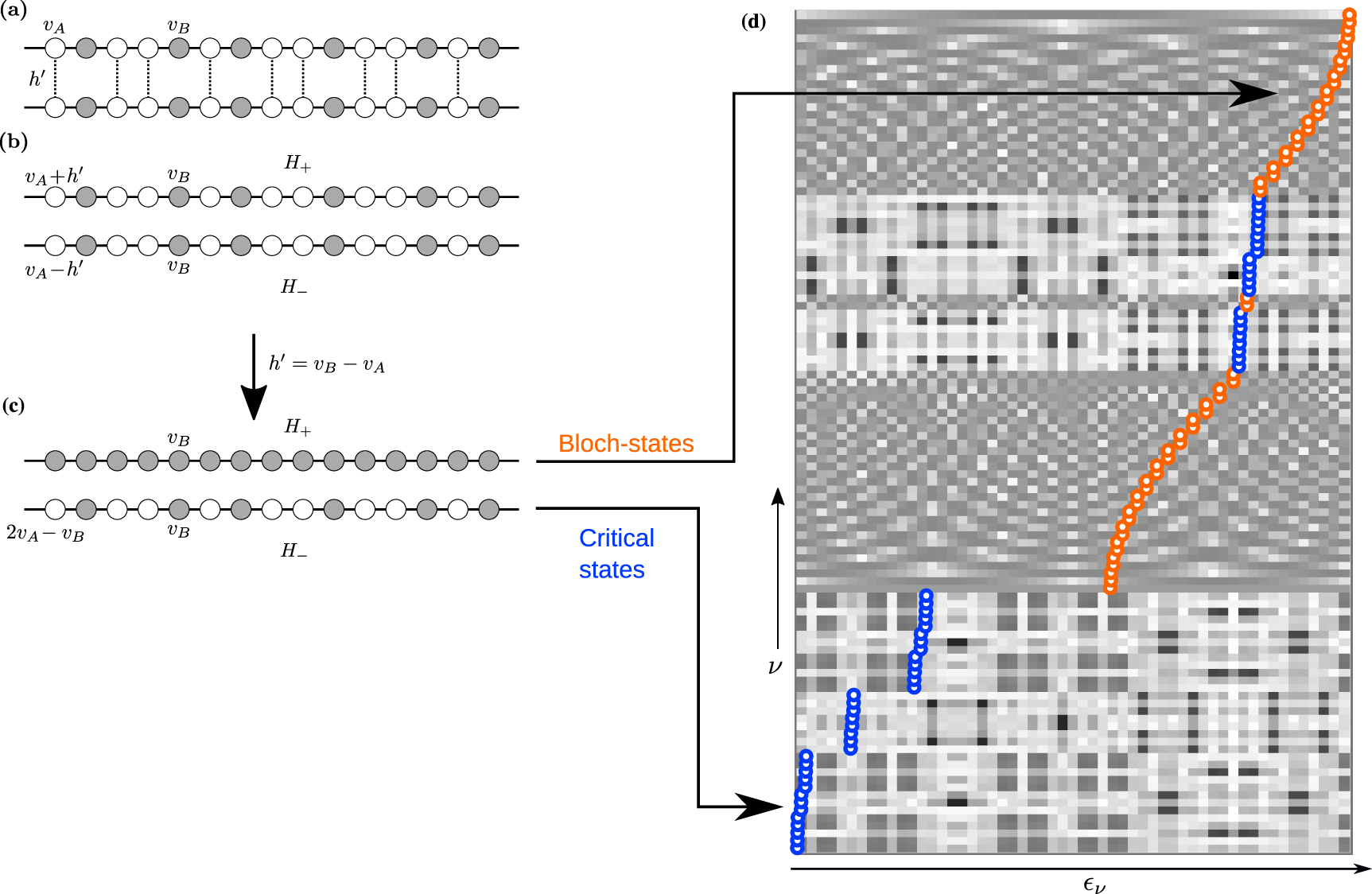
5.1. Coupling only A or only B-sites

In the first case, we couple only the A sites to each other, as depicted in figure 4(a). Repeating the same steps as above, we obtain $H^{^{\prime}} = \mathcal{S}^{-1}H \mathcal{S} = H_{+} \oplus H_{-}$, though now with

$$\begin{equation} H_{\pm} = \sum_{i = 1}^{N} v^{\pm}_{i} \vert i\rangle \langle i\vert + h \sum_{\langle i,j \rangle} \vert i\rangle \langle \,j\vert \end{equation} \tag{ 9 }$$

where $v^{\pm}_A = v_A\pm h^{^{\prime}}$, while $v_B^{\pm} = v_B$ is unchanged (see figure 4(b)). In a completely analogous manner, coupling only the B-sites to each other will result in an energy shift of the on-site potentials of the B-sites only.

Zoom In Zoom Out Reset image size

A particularly interesting case occurs when coupling only the A-sites and setting $h^{^{\prime}} = v_B - v_A$. For this special choice of hʹ, $H_{+}$ becomes a uniform chain with zero on-site potential. However, $H_{-}$ is still a Fibonacci chain. Now, since the eigenstates of $H_{\pm}$ correspond to positive/negative parity eigenstates of the full chain, the system features an interesting combination of traits: while the positive parity eigenstates are extended, the negative parity eigenstates are critical. For a quantum system, this means that the phase diagram of such a Hamiltonian features a special point $h^{^{\prime}} = v_B - v_A$ , at which the system's behavior is highly dependent on the energies of one-particle excitations. As depicted in figure 4(a), depending on the energy of these parity eigenstates, they will either form Bloch waves (orange energy levels), or critical states (blue energy levels). It is interesting to see that a specific point in parameter space shows a mixture of singular continuous and absolutely continuous spectra. This provides a platform where both properties of extended and critical states can be exploited by tuning the Fermi level. In the critical regime, for example, (thermal) conductivities are in general very low (in some cases, they are even lower than for conventional insulators) [27, 28]. On the other hand, the fully extended regime provides the possibility to have phases with high (electrical) conductivities.

Finally, let us note that the possibility of Bloch-states in coupled aperiodic setups has also been observed in references [12, 13], in which more complicated coupling schemes have been used.

5.2. Defect-coupling

Another possibility is the selective coupling of only a small subset of sites. In the extreme case, this subset consists of one site in each chain (see figure 5(a)). The result of such a coupling can be easily deduced. Using the symmetry adapted basis, we see that $H_\pm$ will both be simple Fibonacci chains, with added impurities at the sites that are coupled (see figure 5(b)). Such systems have been analyzed previously, and it was found that a single weak impurity is sufficient to render the spectrum unstable and reduce its fractal dimension, leading to a loss of criticality in all states [29]. On top of that, it was also recently found that this does not affect all states equally. Using Niu's renormalization procedure [9, 18], it was shown that the degree of criticality loss is dependent on the renormalization path of the site at which the impurity is placed [30]. This means that the location of the impurity impacts which states of the unperturbed Fibonacci chain are the most affected.

Zoom In Zoom Out Reset image size

Alternatively, the impact of a single-site defect can be analyzed in a framework of local resonators [22]. These local resonators form building blocks of the whole chain. In an unperturbed (without impurity) chain, each eigenstate is approximately symmetric with respect to a local parity operator. The sites with the highest amplitudes will be the ones corresponding to the resonator structures, which are symmetric under local parity. This approximate symmetry depends on the contrast $c = |h|/|v_A-v_B|$, and is exact in the limit c → 0. By placing an impurity on a particular site, one creates a new local resonator structure in the chain, and as such, new localization properties arise, yielding states with amplitude distributions that are radically different from the rest of the eigenstates. This can be seen in figure 5(c), where the in-gap states have very strong localization, marked by the darker patches around a particular region of the chain (see the topmost level, for example, where there is a very dark patch around site j = 10) around this new local resonator block [22].

Yet another alternative way of coupling the two chains is in a quasiperiodic manner. Out of the many possibilities, here we illustrate an immediate and interesting one: We couple only a subset of B-sites to each other; namely, those appearing in the pattern AABAA, as shown in figure 6(a), where the darker B site sits in between two A sites on each sides. We further set the coupling between the chains to h and choose the coupled B site energy to $v_B^{^{\prime}} = v_B+h$, such that $H_{-}$ becomes a regular Fibonacci chain, with on-site energies v_A and v_B . On the other hand, $H_{+}$ now features new on-site energies: $v_B+2h$, distributed in a quasiperiodic manner. For this choice of coupling, there are $F_{N-5}$ such new sites (which is the number of AABAA blocks in a chain of length F_N ).

Zoom In Zoom Out Reset image size

In analyzing the effective chain using a renormalization approach, we make the assumptions that h < 0 and $v_A\lt v_B$. These assumptions are made to enforce the trifurcating structure necessary for the Fibonacci chain's renormalization group flow.

6.1. Decimation procedure

We can apply the usual decimation procedure known for hierarchical chains [18]. In this case, the novelty lies in the chain with three different on-site energies, as shown for example in figure 7. There are three renormalized chains that result from the first decimation step. We can analyze them separately to see how each energy level splits into different branches. A sketch of the branching structure is shown in figure 8, where one sees that there are three main clusters. The v_C cluster follows the Fibonacci trifurcarting structure from the start. The v_B cluster splits into six levels, each of which starts trifurcating according to the Fibonacci structure. Finally, the v_A cluster splits into seven levels that also trifurcate afterwards. In the thermodynamic limit, these levels keep on trifurcating indefinitely, leading to a spectrum that is a Cantor set and known to be singular continuous [31]. In appendix, we provide a comprehensive explanation of the step-by-step renormalization process involved in handling the binary hoppings T_A and T_B for each cluster. In the next section, we show that these analytic tools lead to a good approximation and understanding of the structure of the spectrum.

Zoom In Zoom Out Reset image size

Zoom In Zoom Out Reset image size

6.2. Effective couplings and energy corrections

In order to calculate the effective couplings and energy corrections at each splitting, we use the Brillouin–Wigner perturbation theory. For each cluster, we use the effective Hamiltonian equation (4)

$$\begin{equation*} H_{\textrm{eff}} = QH_0Q+QH_1\sum_{n = 0}^n\left(P\frac{1}{E-H_0}H_1\right)^nQ, \end{equation*} \tag{ 6.2 }$$

where H₁ is the perturbation corresponding to the weakest coupling, Q is the projector onto the eigenspace of H₀ corresponding to the cluster of interest, while P projects out of it. At first, H₀ is just composed of on-site energies and H₁ of the coupling h between the isolated sites. This results in the three degenerate levels that form the main clusters. In the next order of perturbation theory, H₀ denotes the Hamiltonian of the corresponding renormalized chain, with the weakest coupling turned off. H₁ is then the perturbation with either t_w or t_b turned on, depending on which subchain we are dealing with (i.e. depending on whether $t_b\gt t_w$ or vice-versa). With this effective Hamiltonian for each of the clusters, the renormalized couplings can be found by calculating $\langle E_j\vert H_{\textrm{eff}}\vert E_{j+1}\rangle$, where $\vert E_j\rangle$ are the zeroth order local eigenstates, which are either one atomic site, a two or a four-atom molecule, depending on the situation. We now first state the results obtained from the first-order corrections, which we shall subsequently prove. We find the first three renormalized couplings to be given by

$$\begin{align} (t_b, t_s, t_w) = \begin{cases} \displaystyle\left( \frac{c}{1-2c},\ 1,\ c\right)h, \ \ \ \text{(Cluster A)} \\[8pt] \displaystyle\left(-\frac{c^4}{2} ,\ -c ,\ c^2 \right)h, \ \ \ \text{(Cluster B)} \\[8pt] \displaystyle\left(0,\ -\frac{1}{4}\left[\frac{c}{1-2c}\right]^5,\ \frac{1}{16}\left[\frac{c}{1-2c}\right]^8 \right)h, \ \ \ \text{(Cluster C)} \end{cases} \end{align} \tag{ 10 }$$

where we have defined the contrast parameter $c\equiv |h/(v_A-v_B)|$, which controls how well the perturbation theory behaves. We point out that the physics described by the theory is consistent for

$$\begin{equation} c<\frac{1}{4^{\frac{1}{3}}(1+4^{\frac{1}{6}})}\approx 0.27875, \end{equation} \tag{ 11 }$$

after which it fails to deliver reasonable results. This result will also be proven in the following paragraphs.

6.2.1. First order renormalized hoppings

Figure 9 shows that one can form three effective chains (a), (b) and (c), corresponding to the clusters v_A , v_B and $v_C = v_B+2h$ respectively. Before deriving our results, we recall that we are working in the regime of parameters where $v_A\lt v_B$ and h < 0. This is done to obtain a hierarchy of hopping strengths that will result in the infinitely trifurcating structure after (at most) the second renormalization step. The v_C cluster is a regular hopping Fibonacci chain. In fact, if one starts from a chain of generation N, with F_N sites, one ends up with one of generation N − 5, with $F_{N-5}$ sites. By calculating the matrix element $\langle E_j\vert H_{\textrm{eff}}\vert E_{j+1}\rangle$, where H_eff is given by equation (4), between the nearest neighboring eigenstates of the unperturbed Hamiltonian H₀ in the $E = v_C$ subspace, we find that this chain has effective renormalized hoppings, to nearest order in the contrast $c = |h|/|v_A-v_B|$, given by

$$\begin{equation} \begin{split} t_s& = \frac{h^6}{4(v_B-v_A+2h)^5} = -\frac{1}{4}\left[\frac{c}{1-2c}\right]^5h, \\ t_w& = \frac{1}{16}\frac{h^9}{(v_B-v_A+2h)^8} = \frac{1}{16}\left[\frac{c}{1-2c}\right]^8h. \end{split} \end{equation} \tag{ 12 }$$

Zoom In Zoom Out Reset image size

Next, we consider the v_B chain, which contains six clusters. Two clusters correspond to the two-atom molecule bonded by t_s , while the other four correspond to the four-atom molecule (composed of two two-atom molecules bonded by $|t_w|\gt|t_b|$). These clusters will further start to trifurcate because they end up having the structure of a hopping Fibonacci chain after decimation. The renormalized hoppings of this chain are given by

$$\begin{equation} \begin{split} t_b& = \frac{-h^5}{2(v_B-v_A)^4} = -\frac{c^4}{2}h, \\ t_s& = \frac{h^2}{v_B-v_A} = -ch, \\ t_w& = \frac{h^3}{(v_B-v_A)^2} = c^2h. \end{split} \end{equation} \tag{ 13 }$$

Finally, we consider the v_A cluster. It has seven clusters. The six clusters come from the same structures as the v_B chain, i.e two- and four-atoms molecules, and the additional cluster comes from isolated sites. Once again, each one of these clusters will start trifurcating at the next steps of decimation, and one retrieves the hopping Fibonacci chain structure. The renormalized hoppings of this chain are

$$\begin{equation} \begin{split} t_b& = \frac{h^2}{v_A-v_B-2h} = \frac{c}{1-2c}h,\\ t_s& = h, \\ t_w& = \frac{h^2}{v_A-v_B} = ch. \end{split} \end{equation} \tag{ 14 }$$

6.2.2. Regime of validity of the perturbation theory

Let us now study the regime of validity which results in the hopping hierarchy discussed previously. Starting with the v_B subspace, which is the simplest to deal with, we see from equation (13) that the hierarchy $|t_s|\gt|t_w|\gt|t_b|$ will always hold for $c\in(0,1)$. This immediately results in the trifurcating structure after one iteration of the renormalization procedure. The v_A subspace, on the other hand, restricts the range of c further. In order to have $|t_s|\gt|t_b|\gt|t_w|$, we must impose

$$\begin{equation*} 1>\left|\frac{c}{1-2c}\right|>c \end{equation*}$$

which leads to $0\lt c\lt1/3$. Finally, the v_C subspace will give us the final restriction to impose the hierarchy leading to a trifurcating structure. This means we want $|t_s|\gt|t_w|$, leading to

$$\begin{equation*} \frac{1}{4}\left|\frac{c}{1-2c}\right|^5>\left|\frac{c}{1-2c}\right|^8. \end{equation*}$$

Solving for c > 0 yields the final restriction

$$\begin{equation} c<\frac{1}{4^{\frac{1}{3}}(1+4^{\frac{1}{6}})}. \end{equation} \tag{ 15 }$$

6.2.3. Energy corrections

We also determined the first-order energy corrections using the same perturbation theory, and found the spectrum shown in figure 10. The energy levels calculated using perturbation theory (in blue) and those from numerical direct diagonalization (in red) have the same structure, with some discrepancies that disappear as the contrast c → 0. This is illustrated in figures 10(a) and (b) with $c = 1/4$ and $c = 1/8$, respectively. The structure of the spectrum is well approximated by the theory, even for a small chain size of 21 sites. The exact expressions for the energy levels can be found in table 1 .

Zoom In Zoom Out Reset image size

Table 1. The first order correction to the three clusters v_A , v_B and $v_B+2h$. Any higher order correction will further split each of these energies into three, with corrections given by $\pm T_A$ and 0 (see appendix for the values of T_A in each case). Each of the three levels again will split into three and so on, with the well known spectrum structure of the hopping Fibonacci chain.

E0	E1
vA	$\frac{1}{\sqrt{2}}\sqrt{t_b^2+2t_s^2+\sqrt{(t_b^2+2t_s^2)^2-4t_s^4}}$
	$\frac{1}{\sqrt{2}}\sqrt{t_b^2+2t_s^2-\sqrt{(t_b^2+2t_s^2)^2-4t_s^4}}$
	ts
	0
	$-t_s$
	$\frac{1}{\sqrt{2}}\sqrt{t_b^2+2t_s^2+\sqrt{(t_b^2+2t_s^2)^2-4t_s^4}}$
	$-\frac{1}{\sqrt{2}}\sqrt{t_b^2+2t_s^2-\sqrt{(t_b^2+2t_s^2)^2-4t_s^4}}$
vB	$\frac{1}{\sqrt{2}}\sqrt{t_b^2+2t_s^2+\sqrt{(t_b^2+2t_s^2)^2-4t_s^4}}$
	$-\frac{1}{\sqrt{2}}\sqrt{t_b^2+2t_s^2-\sqrt{(t_b^2+2t_s^2)^2-4t_s^4}}$
	ts
	$-t_s$
	$-\frac{1}{\sqrt{2}}\sqrt{t_b^2+2t_s^2+\sqrt{(t_b^2+2t_s^2)^2-4t_s^4}}$
	$-\frac{1}{\sqrt{2}}\sqrt{t_b^2+2t_s^2-\sqrt{(t_b^2+2t_s^2)^2-4t_s^4}}$
$v_B+2h$	ts
	0
	$-t_s$

Now, one only needs to add the spectrum of the regular chain to this 'modified' chain to obtain the full spectrum of the two connected chains, as shown in figure 11.

Zoom In Zoom Out Reset image size

In the following, we consider a case where the two Fibonacci chains are not coupled directly, but instead through intermediate sites. Before we start, let us first investigate a setup where two periodic chains are coupled indirectly, as shown in figure 12(a). In figure 12(b), we depict the band structure of this so-called 'one-dimensional Lieb lattice' [32]. What makes this lattice interesting is that, among four dispersive bands, it also features one completely flat band fulfilling $E(k) = \text{constant}$ for all k. This defining feature of flat bands renders them dispersionless; they suppress wave transport [33]. On the other hand, the density of states in a flat band diverges, so that any disorder or non-linear effects may qualitatively change the transport properties [33, 34]. Moreover, in lattices where the single-particle Hamiltonian features a flat band, even arbitrarily weak interactions may act non-perturbatively. This can lead to boson pair formation [35–37] or other interesting phases, such as the Haldane insulator [38] and Wigner crystals [39].

Zoom In Zoom Out Reset image size

In two dimensions, a classical example for a system with flat bands is the Lieb lattice, whose structure is very similar to the system depicted in figure 12(a). The two-dimensional Lieb lattice has been realized in a number of different experimental platforms, such as tailored atomic structures on substrates [40, 41], evanescently coupled waveguide arrays [42, 43], terahertz spoof plasmons [44], or cold atom setups [45, 46]. Interestingly, the CuO₂ planes in high-temperature cuprate superconductors possess a Lieb lattice structure, and it has been conjectured that flat bands might play a role in their high critical temperature [33, 47–51].

Flat bands are also interesting from another perspective, since they are tightly connected to the emergence of a special kind of eigenstates, the so-called 'compact localized state' (CLS) [52–54]. For the one-dimensional Lieb lattice, a CLS is shown in figure 12(a), consisting of an excitation of only four B sites. The CLS thus 'lives' only on a single plaquette (marked by a dotted rectangle) and strictly vanishes outside it. In other words, it is perfectly localized on a very small part of the setup.

The defining feature of CLSs—namely, their perfect localization—renders these states very robust against perturbations: Since they vanish exactly outside their localization domain $\mathcal{D}$, they are not affected by any changes to the system outside $\mathcal{D}$. Due to this property, CLSs are ideal candidates for storing information [55, 56]. The perfect localization of CLSs might further be interesting in the context of photonic waveguide arrays, where it allows for diffraction-free transmission of information in the form of CLSs [42, 57].

After the above considerations, let us now couple two aperiodic Fibonacci chains in an indirect manner. Out of the many possibilities, here we choose one of the simplest, yet quite interesting setup, depicted in figure 12(c). Each A-site of the upper chain is coupled by an intermediate B-site to its counterpart A-site on the lower chain. This setup also features a macroscopic number of CLSs, one of which is depicted in figure 12(c).

When comparing the one-dimensional version of the Lieb lattice [58, 59]—shown in figure 12(a)—to the coupled Fibonacci chains depicted in figure 12(c), one sees that they are rather similar. Due to this high similarity, we call the coupled Fibonacci setup of figure 12(c) the 'quasiperiodic Lieb lattice'. The similarity in the structure of the two lattices is also visible in their eigenvalue spectra, since both lattices feature a flat (quasi) band. The emergence of this flat band can easily be understood, since (for an infinite setup) there is an infinite number of plaquettes, and thus an infinite number of degenerate CLSs. In both cases, the flat bands emerge due to destructive interference [33].

In this work, we analyzed various ways of coupling two identical Fibonacci chains to each other. The main tool that helped us to identify the features of these systems is a symmetry adapted block-diagonalization of the Hamiltonian H into $H_+\oplus H_-$. Once we find the eigenstates of $H_\pm$, we can symmetrize/anti-symmetrize them, respectively, to obtain the eigenstates of the original Hamiltonian H. In addition, the eigenvalue spectrum of the system is simply given by a multiset sum of the eigenvalue spectra of the blocks $H_\pm$.

After briefly introducing the individual Fibonacci chain, we started by exploring the effects of uniformly coupling two identical chains. We then found that the resulting eigenvalue spectrum is just a sum of two shifted Fibonacci spectra, which renders the behaviour of a particle in such a system identical to that in a conventional Fibonacci chain. We have subsequently explored the case of a nonuniform coupling, where we coupled only A (or only B) sites. An interesting scenario occurs when the interchain coupling is $h^{^{\prime}} = v_B-v_A$, since $H_+$ then becomes a periodic chain, for which the eigenstates are Bloch waves. On the other hand, $H_-$ is still a Fibonacci chain, such that the complete spectrum offers a mixture of critical and fully extended eigenstates, identifiable by the parity of the corresponding wavefunctions. The next type of coupling that we have analyzed is between a small subset of sites, i.e. a so called defect coupling, leading to block Hamiltonians $H_\pm$ which are Fibonacci chains with on-site defects. This has been followed by another interesting and more complicated case of quasiperiodically coupled chains. The resulting block Hamiltonians could be thought to be like several coupled defects, but we have shown, through a perturbative renormalization analysis, that all states in this chain belong to the same family of critical states. Finally, we explored two Fibonacci chains coupled to each other in the same manner as the nonuniform coupling of section 5, but with an intermediate site in between. This offers the possibility of having a set of CLSs, leading to a flat bland in the energy spectrum. Overall, the demonstrated emergence of CLSs in the quasiperiodic Lieb lattice represents an interesting addition to the existing literature on these phenomena in quasiperiodic setups (see, for instance, [60–62]). Two immediate tasks for the near future would be to analyze the quasiperiodic Lieb lattice in the context of interacting electrons, or to investigate the impact of (correlated) disorder on the transport properties.

This publication is part of the project TOPCORE with Project Number OCENW.GROOT.2019.048, which is financed by the Dutch Research Council (NWO). This work (P S) is supported by the Cluster of Excellence 'Advanced Imaging of Matter' of the Deutsche Forschungsgemeinschaft (DFG) - EXC 2056 - Project ID 390715994.

All data that support the findings of this study are included within the article (and any supplementary files).

In the next subsections, we will determine the energy corrections and the renormalized Fibonacci hoppings for each cluster.

Appendix.  v_A cluster

Starting with the v_A cluster, we can split it into the three categories depicted in figure A1. The 4-atom molecule leads to four energy eigenvalues,

$$\begin{equation} E^A_{4M} = \pm\frac{1}{\sqrt{2}}\sqrt{t_b^2+2t_s^2\pm\sqrt{(t_b^2+2t_s^2)^2-4t^{\,4}_s}}, \end{equation} \tag{ A.1 }$$

where the subscript 4M reminds us that it is for the 4-atom molecule, while the superscript A indicates that it applies to the initial level v_A . The 2-atom molecule and the isolated atom have eigenvalues, respectively, equal to

$$\begin{align} E^A_{2M}& = \pm t_s, \end{align} \tag{ A.2 }$$

$$\begin{align} E^A_A& = 0. \end{align} \tag{ A.3 }$$

Zoom In Zoom Out Reset image size

In order to calculate the effective hoppings using the Brillouin-Wigner degenerate perturbation theory, we need to know the eigenstates of H^A ₀, which for the $E_A^A = 0$ level are just the corresponding isolated sites. For the 2-atom molecules, these are given by $\vert E^A_{2M}\rangle = 2^{-1/2}(\vert i\rangle \pm\vert i+1\rangle )$ for some localized one-particle state at site number i, corresponding to the sites coupled by the strongest bond, and for the 4-atom molecules

$$\begin{equation*} \vert E^A_{4M}\rangle = \frac{a_0\vert i\rangle +a_1\vert i+1\rangle +a_2\vert i+2\rangle +a_3\vert i+3\rangle }{\sqrt{a^2_0+a_1^2+a_2^2+a_3^2}} \end{equation*}$$

for the relevant sites i to i + 3, as shown in figure A1. The coefficients can be computed by solving the eigenvalue problem

$$\begin{equation*} \begin{pmatrix} 0 & t_s & 0 & 0 \\ t_s & 0 & t_b & 0 \\ 0 & t_b & 0 & t_s \\ 0 & 0 & t_s & 0 \end{pmatrix}\begin{pmatrix} a_0 \\ a_1 \\ a_2 \\ a_3 \end{pmatrix} = E_{4M}\begin{pmatrix} a_0 \\ a_1 \\ a_2 \\ a_3 \end{pmatrix}. \end{equation*}$$

A solution to this problem is

$$\begin{equation} \begin{aligned} a_0& = 1, & a_1& = \frac{E_{4M}}{t_s}, \\ a_2& = \frac{E^2_{4M}-t_s^2}{t_bt_s}, & a_3& = \frac{E_{4M}}{t_s}\frac{E^2_{4M}-t_s^2-t_b^2}{t_bt_s}, \end{aligned} \end{equation} \tag{ A.4 }$$

where we ommited the superscript A for brevity. Each of the degenerate subspaces can be associated to its own chain, with its own couplings in the renormalization picture (see figure A1).

The effective Hamiltonian for the v_A cluster is found by setting the perturbation Hamiltonian H₁ to be the one with all matrix elements containing t_w . We remind the reader that the general expression was given by equation (6.2).

$\boldsymbol{E_{4M}}$ chain (cyan)

The couplings in the 4-atom molecular chain are given by the matrix element $\langle E^{A}_{4M,j}\vert H^{A}_{eff}\vert E^{A}_{4M,j+1}\rangle$, where j is the renormalized site index. To nearest order in t_w , they read

$$\begin{equation} \begin{aligned} T_A& = \frac{a_3}{N}\frac{t_w^2}{E_{4M}}, \\ T_B& = \frac{a_3}{N}\frac{t_w^4t_s}{E^2_{4M}(E^2_{4M}-t_s^2)}, \end{aligned} \end{equation} \tag{ A.5 }$$

where we defined $N\equiv a_0^2+a_1^2+a_2^2+a_3^2$. Note that there are four different $E_{4M}$'s and hence four sets of coefficients a.

$\boldsymbol{E_{2M}}$ chain (blue)

The 2-atom molecular chain's couplings are obtained from the matrix elements $\langle E^{A}_{2M,j}\vert H^{A}_{eff}\vert E^{A}_{2M,j+1}\rangle$. The calculation yields

$$\begin{equation} \begin{aligned} T_A& = \pm\frac{t_w^4}{2t_s^2}\sum_{j = 0}^3\frac{a_3^{(j)}}{N_j\left(\pm t_s-E^{(j)}_{4M}\right)}, \\ T_B& = \frac{t_w^6}{2t_s^3}\left(\sum_{j = 0}^3\frac{a_3^{(j)}}{N_j\left(\pm t_s-E^{(j)}_{4M}\right)}\right)^2, \end{aligned} \end{equation} \tag{ A.6 }$$

where we have now explicitely given a label to each of the four sets of a_j 's, and by extention, N_j 's as well. The ± refers to the bonding and anti-bonding energy levels.

$\boldsymbol{E_{A}}$ chain (green)

Finally, the isolated atom chain has the following couplings

$$\begin{equation} \begin{aligned} T_A& = -\frac{t_w^2}{2t_s}, \\ T_B& = -t^{\,2}_w \sum_{j = 0}^3\frac{a_3^{(j)}}{N_jE^{(j)}_{4M}}. \end{aligned} \end{equation} \tag{ A.7 }$$

Appendix.  v_B cluster

For the v_B cluster's effective chains, we only have two categories, as shown in figure A2. The first (cyan) corresponds to a 4-atom molecular chain, with the same energy eigenvalues and eigenstates formulae as the previous ones, but with a different set of $\{t_b,t_s,t_w\}$ (see equation (10)). The second (blue) subchain corresponds to the 2-atom molecular chain. We shall, once again, refer to them as the $E_{4M}$ and $E_{2M}$ chains, respectively.

Zoom In Zoom Out Reset image size

$\boldsymbol{E_{4M}}$ chain

The couplings in this case are given by

$$\begin{equation} \begin{aligned} T_A& = \frac{t_w}{N}a_3, \\ T_B& = \frac{a_3}{N}\frac{t_w^2t_s}{E_{4M}^2-t_s^2}. \end{aligned} \end{equation} \tag{ A.8 }$$

$\boldsymbol{E_{2M}}$ chain

The couplings for this chain are

$$\begin{equation} \begin{aligned} T_A& = \pm\frac{t_w^2}{2}\sum_{j = 0}^3\frac{a_3^{(j)}}{N_j\left(\pm t_s-E_{4M}^{(j)}\right)}, \\ T_B& = \pm\frac{t_w^{\,3}}{2}\left(\sum_{j = 0}^3\frac{a_3^{(j)}}{N_j\left(\pm t_s-E_{4M}^{(j)}\right)}\right)^2. \end{aligned} \end{equation} \tag{ A.9 }$$