


Abstract
Characterization of an isolated attosecond pulse (IAP) in the extreme ultraviolet (XUV) or soft x-ray (SXR) region is essential for its applications. Here we propose to retrieve an IAP in the time domain directly through the modulation of high-harmonic generation (HHG) spectra in the presence of a time-delayed intense few-cycle infrared or mid-infrared laser. The retrieval algorithm is derived based on the strong-field approximation and an extended quantitative rescattering model. We show that both isolated XUV pulses with a narrow spectral bandwidth and isolated SXR pulses with a broad bandwidth can be well characterized through the HHG streaking spectra. Such an all-optical method for characterizing the IAP differs from the commonly used approach based on the streaked photoelectron spectra that would require electron spectrometers. We check the robustness of the retrieval method by changing the dressing laser or by adjusting the steps of time delay. We also show that the XUV pulse can be accurately retrieved by treating the HHG streaking spectra calculated from solving the time-dependent Schrödinger equation for single atoms as the 'experimental' data.
Export citation and abstract BibTeX RIS

Original content from this work may be used under the terms of the Creative Commons Attribution 4.0 license. Any further distribution of this work must maintain attribution to the author(s) and the title of the work, journal citation and DOI.
1. Introduction
In the past few decades, the rapid development of high-harmonic generation (HHG) technique has provided effective laboratory light pulses for probing the ultrafast electronic dynamics of atoms, molecules and solids [1–4]. These light pulses can be in the form of attosecond pulse trains [5] or isolated attosecond pulses (IAPs) [6], are instrumental to the birth of attosecond science since 2001. Taking advantage of their better temporal resolution, much effort has been paid to the generation of IAPs. There have been a number of established gating methods to produce IAPs in the extreme ultraviolet (XUV) region with duration ranging from a few hundreds to a few tens attoseconds, including amplitude gating [7], ionization gating [8], polarization gating [9], double-optical gating [10], attosecond lighthouse [11, 12], multi-color waveform synthesis [13–15], and phase-matching in the overdriven regime [16, 17]. Beginning around 2011, with the development of mid-infrared (MIR) laser technology [18], several groups have generated continuum harmonic spectra [19–23] in the soft x-ray (SXR) region and a few have reported the characterization of their temporal behaviors [24–28]. These SXR pulses have a much broader spectral bandwidth and potentially shorter pulse durations. For example, an IAP as short as 53 as was reported for a spectral bandwidth of 100–300 eV driven by a two-cycle 1.8 µm laser [26]. A prerequisite for wide applications of attosecond pulses is to know accurately their temporal information, but the actual characterization is seldom done because the method is complicated. Therefore, it is desirable to develop other practical methods to characterize IAPs in the XUV to SXR regions.
Similar to femtosecond laser pulses, one can use autocorrelation [24, 29] to measure the duration of IAP. However, this method cannot give the temporal waveform. To fully characterize an IAP, its spectral phase and amplitude over the whole bandwidth is needed. The common one is the so-called attosecond streaking method [30]. In this method, modulated continuum photoelectron spectra are measured by ionizing an atomic target using a single attosecond XUV pulse in the presence of a moderately intense infrared (IR) laser by varying the time delay between the two pulses. The frequency-resolved optical gating for complete reconstruction of attosecond bursts (FROG-CRABs) [31–33] has been most frequently used to retrieve the isolated XUV attosecond pulse with the photoelectron streaking spectra. However, FROG-CRAB is intrinsically limited to small bandwidth of a few tens of electron volts. For broader bandwidths, other methods have been proposed, such as principal component generalized projections algorithm [34], phase retrieval by omega oscillation filtering [35], Volkov-transform generalized projection algorithm [36], and extended ptychographic iterative engine [37]. In recent years, phase retrieval of broadband pulses method has been developed [38–40] which can retrieve narrow-bandwidth XUV pulses more accurately than the FROG-CRAB. More importantly, it can be used to retrieve broadband SXR IAPs with the MIR laser as the streaking field. It has also been modified to include photoelectrons over a large angular range to improve the statistics of signals [41] and to characterize single-shot attosecond pulses generated at x-ray free-electron facilities [42]. In the latter case, the IAP is different in each single shot and the streaking IR field is circularly polarized where two-dimensional or three-dimensional electron momentum spectra are measured. Very recently, Witting et al [43] reported on the full characterization of XUV attosecond pulses generated by near-single-cycle pulses at a repetition rate of 100 kHz by using the streaking global optimization method. Xue et al [44] used the attosecond streaking measurement to demonstrate a gigawatt, 226 as isolated pulse in the spectral region of 50–70 eV from a low-repetition rate, three-channel waveform synthesizer by using FROG-CRAB. Furthermore, cutting-edge machine learning technology has also been employed to reconstruct the attosecond pulse with several neural networks, such as conditional variational generative network [45], deep neural network, and convolutional neural network [46].
The methods above are all based on measuring photoelectron streaking spectra. Alternatively, several all-optical methods have been proposed to characterize attosecond pulses. For example, Dudovich et al [47] applied a low-intensity second-harmonic beam to gently perturb the harmonic spectra generated by the intense IR laser. The duration of the attosecond pulse is reconstructed from the modulation of even-harmonic signals as a function of the delay between two fields. Kim et al [48] used a second-harmonic beam with time-dependent polarization as a perturbing pulse for the IAP generated by the IR laser such that far-field XUV intensity distribution is modulated. This is then used to determine the amplitude and phase of the IAP. In addition, Xue et al [49] theoretically investigated the dependence of the spectral modulation on the chirp of the XUV under synchronized XUV and IR laser pulses, which could be used to reconstruct the XUV spectral phase. Recently, Yang et al [50] used a weak field to perturb the harmonic emission so that the accumulated phase of the electron trajectory can be altered. Since the perturbed harmonic spectrum can be formulated as a convolution of the unperturbed dipole and a phase gate, the conventional frequency-resolved optical gating (FROG) method is thus applied to completely retrieve the IAP. Two years later, the same group developed an all-optical attosecond time domain interferometry by using the similar generation scheme for the perturbed HHG [51]. Meanwhile, in 2020, Sarantseva et al [52] proposed to retrieve the temporal intensity profile of an XUV attosecond pulse based on the XUV-assisted HHG by an intense IR pulse. These all-optical methods in general have some advantages. Compared to the attosecond photoelectron streaking method, the measurement setup is the same as that for the HHG, and the optical signal has higher resolution than the electron signal. Therefore, it is highly desirable to develop all-optical methods to characterize IAPs from the XUV to SXRs.
In this work, our main goal is to develop an algorithm for reconstructing the spectral phase of IAP by using the modulated features in the all-optical HHG streaking spectra. This algorithm is based on the strong-field approximation (SFA) and an extended quantitative rescattering (EQRS) model. In our scheme, a weak XUV (or SXR) IAP pulse is used to modulate the continuous harmonic spectra in its spectral range generated by an intense dressing few-cycle IR (or MIR) laser. Here the name of 'all-optical HHG streaking' is used to indicate both the similarity as well as the distinction with respect to the commonly used attosecond photoelectron streaking. The spectral modulation can be controlled by adjusting the time delay between the XUV (or SXR) and IR (or MIR) laser pulses. Note that this scheme can be easily implemented in the experiment by using the same generation setup as that for the attosecond photoelectron streaking spectra while the measurement setup is replaced by that for the HHG. It can also be realized by other setups, for instance, two gas-jet setup employed by Seres et al [53, 54]. In our previous work [55], a simpler approach was introduced to characterize the IAP where the spectral phase can be described by a single parameter only. The parameter was retrieved through iterative procedure. In section 2, we will present the main ingredients of EQRS model and will derive the algorithm for retrieving the spectral phase of IAP. In section 3, we first will test the validity of retrieval algorithm, next will show a few examples of retrieving isolated XUV and SXR pulses, then will check the robustness of retrieval algorithm by varying the intensity of dressing laser and by changing the step size of the time delay. Finally, we will examine the retrieval method by using the HHG streaking spectra from solving the time-dependent Schrödinger equation (TDSE). The article will be summarized in section 4. Atomic units and the atomic target of Ne are used unless noted otherwise.
2. Theoretical methods
2.1. EQRS model
To simulate single-atom HHG streaking spectra under a linearly polarized weak XUV (or SXR) IAP and a strong IR (or MIR) laser, we can employ the previously established EQRS model [55]. This model is an improvement of SFA [56]. In the SFA, the single-atom induced dipole along the polarization direction at a fixed time delay τ between the two pulses can be written as

where pst
is the canonical momentum, Sst
is the quasi-classical action,  is the combined electric field of IR and XUV pulses, and
  is the corresponding vector potential. Note that negative τ means the XUV pulse comes earlier than the peak of IR laser. Here equation (1) is expressed for IR and XUV pulses, but also can be used for MIR and SXR pulses.
Different terms in the time-dependent dipole  can be separated in the following:

Each term in the right hand of the equation can be explicitly expressed as
and
where f(p) is related to the dipole transition matrix element d(p) from the ground state to a continuum state as  with electron momentum p and the stationary action
  without including the effect of the XUV pulse is

Note that the  term gives the induced dipole solely by the IR laser, the
  term is by the XUV pulse alone, and the
  and
and  terms give the coupling effect between the two pulses.
The first three terms on the right side of equation (2) in frequency domain can be factorized as


and

where  is the wave packet of the return electron driven solely by the IR laser.
  are complex quantities similar to the electron wave packet in
  and only depend on the external field. Here the peak intensity I of the dressing IR laser is explicitly expressed in the equations. With the same idea of quantitative rescattering (QRS) model [57, 58], ionization probability
  and transition dipole moment
  under the SFA are replaced by the 'exact' values of
  and
and  in the QRS and EQRS models. The ionization probability
  can be calculated by using the PPT model [59], and
  is computed by using the 'exact' wave function for the bound and continuum states within the single-active electron (SAE) approximation. Thus, in the EQRS model, the single-atom induced dipole by the XUV and IR pulses at a time-delay τ can be computed from

In the above equation, the  term is neglected because of its much smaller amplitude. Details of the derivation of EQRS model can be found in [55].
Note that HHG spectra obtained from equation (11) modulate as a function of τ. We have checked that such modulation appears also from TDSE-based harmonic spectra, and thus should be also from the experiment. Detail about the TDSE simulations can be seen in section 3.5.
2.2. Reconstruction of the IAP spectral phase through the time-delayed HHG streaking spectra
When retrieving the spectral phase of XUV pulse from the HHG streaking spectra, we assume that the IR laser pulse and the spectral distribution of the XUV pulse are known. We do not need to know the exact intensity of the XUV pulse, and it is assumed weak, but strong enough to modulate the HHG spectra. The XUV pulse in the frequency domain without the time delay can be expressed as

Here  is the spectral amplitude, and
  is the spectral phase to be retrieved. We assume that the XUV pulse is composed of multiple sub-pulses in the frequency domain. Thus, it can be expanded as in the following:
in which


where  is a Gaussian envelope centered at ωi
with the full-width-at-half-maximum (FWHM) value of Di
and the amplitude of εi
. In equation (14), the XUV spectral phase
is a Gaussian envelope centered at ωi
with the full-width-at-half-maximum (FWHM) value of Di
and the amplitude of εi
. In equation (14), the XUV spectral phase  is maintained, and it can be expanded into terms of a Taylor series about the central frequency ωi
. For the i-th component, it can be written as
is maintained, and it can be expanded into terms of a Taylor series about the central frequency ωi
. For the i-th component, it can be written as

Here the constant term  is the carrier-envelope phase (CEP), and the linear spectral phase term
  is a constant group delay (GD) time.
By taking the Fourier transform of the i-th XUV field  in the frequency domain, it becomes

And its temporal expression can be written as

The derivation of equation (18) is presented in

Note that temporal fields in equations (18) and (19) are expanded using Gaussian envelope basis functions, the temporal form of IAP pulse can be arbitrary.
We have checked that for a spectral region overlapped with the XUV pulse,  is about one order of magnitude smaller than
  , thus the modulated HHG spectra are mainly caused by the interference of x1 and x2 terms. We have checked that this conclusion does not depend on the parameters of the IR laser, the XUV pulse, nor on the atomic target. In equation (4), we assume that all terms involving the IR laser in the integral change slowly over the integration interval in comparison with the vector potential of
  such that the IR electric field can be pulled out from the integral. Thus, under the adiabatic approximation, equation (4) is simplified to

where CIR is a constant related to the IR laser. With the integral in the following

we can obtain

The wave packet  in equation (9) is the same in the SFA and EQRS [55], thus equation (22) is valid in the EQRS model. Multiplying by
  and then integrating both sides of equation (22) with time t, we get

Only when  , the right hand of above equation has a non-zero value. We thus get the following relation:

The derivation of equation (24) can be found in

The derivation of equation (25) is given in

We assume that the CEP of IR laser pulse is zero. The variation of the CEP only leads to a linear term difference in the reconstructed phase, which does not alter the temporal shape and the duration of IAP pulse. For a given ωi
, the maximum of  is reached by varying τ when
  is zero such that the
  reaches its maximum, and we label the satisfied delay time as τi
. Thus, we have
reaches its maximum, and we label the satisfied delay time as τi
. Thus, we have

If the  is small enough, we replace the discrete ωi
and τi
by variables ω and
is small enough, we replace the discrete ωi
and τi
by variables ω and  by omitting the subscript i. Equation (27) is rewritten as

Thus the spectra phase of XUV pulse can be obtained in the following:

For convenience,  at the boundary frequency is set as an arbitrary constant φs
so that
at the boundary frequency is set as an arbitrary constant φs
so that  at the central frequency of XUV pulse is equal to zero.
Note that the spectral phase of XUV pulse can be retrieved from the time-delayed spectra of  . The HHG streaking spectra in the interested spectral region are mainly resulting from the interference of x1 and x2 terms. The former one does not depend on τ, thus for a given ω, the maximum of
  along τ is in coincidence with the maximum in the envelope of HHG streaking spectra. This forms the basis for retrieving the spectral phase of XUV pulse from the time-delayed HHG streaking spectra.
3. Results and discussion
3.1. Validity test of the phase retrieval algorithm
We first check the validity of equation (26) through two numerical examples. In the simulations, the IR pulse has a central wavelength of 800 nm, a FWHM duration of 5 fs, and a CEP of zero. The IR peak intensity of 2.5 × 10¹⁴ W cm−2 provides a sufficient spectral range to cover the XUV pulse with a central photon energy of 71.3 eV and a spectral width of 9 eV. We choose two different phases of XUV pulse as shown in figure 1(a) together with their spectral intensities (assuming a Gaussian distribution and the same for both cases). They correspond to the transform-limited (TL) and chirped XUV pulses, respectively. The peak intensity of the two XUV pulses is 2.5 × 10¹¹ W cm−2, and their temporal profiles are plotted in figure 1(b).

Figure 1. (a) The spectral phases and intensity and (b) the temporal intensity envelopes of XUV pulses. (c) and (d) The spectra of  calculated by using the EQRS model. Note that dotted (black) closed curves indicate the time delays at which the spectra intensity is decreased to 40% of the peak value at each frequency. (e) and (f) Spectral intensities of
  (dashed lines), intensity profiles of
  (solid lines), and (g), (h) time-delayed HHG streaking spectra of
  from equation (11) at three selected photon energies. The XUV pulse is transform limited (TL) (c), (e) and (g) or chirped (d), (f) and (h).
Download figure:
Standard image High-resolution imageWe show the spectra of  calculated by the EQRS model in figures 1(c) and (d). The dotted (black) closed curves are the contour lines indicating the time delays where the spectral peak intensity decrease to its 40% for each given ω. The dashed (white) lines label the peak positions of spectra in terms of
  in equation (28). One can see that the shapes of spectra are greatly modified by the spectral phase of the XUV pulse. We choose three photon energies: 67.5 (blue), 71.5 (black), and 75.5 eV (red), and plot the spectra of
  as a function of the time delay in figures 1(e) and (f). We also show the profiles of
  (dashed lines) in these figures, where αi
is obtained by equation (27). It is clearly shown that the peak of
(dashed lines) in these figures, where αi
is obtained by equation (27). It is clearly shown that the peak of  always agrees with that of the intensity envelope of the shifted IR laser by varying the photon energy and the XUV phase. Thus, equation (26) is verified. Next, we show the modulated HHG spectra resulting from the interference of x1 and x2 terms in figures 1(g) and (h). They have similar envelope shapes in comparison with those of
  , and their peaks appear at the same positions as
  . Therefore, the relation of the GD time αi
and the time delay τ of peak intensity can be set through the HHG streaking spectra. This fact will be used to retrieve the spectral phase of XUV pulse. Note that in the retrieval the complete HHG streaking spectra are used, not from the
. Therefore, the relation of the GD time αi
and the time delay τ of peak intensity can be set through the HHG streaking spectra. This fact will be used to retrieve the spectral phase of XUV pulse. Note that in the retrieval the complete HHG streaking spectra are used, not from the  term only.
3.2. Retrieval of narrow-bandwidth XUV IAPs
We next demonstrate how to retrieve the spectral phase (or temporal profile) of XUV isolated pulse with a narrow bandwidth from the HHG streaking spectra. Such spectra are first simulated by using the EQRS model with known parameters. The parameters of IR laser and XUV pulses are the same as those in figure 1 except for a variety of XUV phase. We assume that the spectral phase of the XUV pulse can be written as

where ω0 is the central frequency,  is a constant, α describes the group delay, β is the coefficient of the group delay dispersion (GDD), and γ accounts for the third-order dispersion (TOD). By choosing different values of these parameters, we can construct five different forms of the spectral phase as shown in figure 2(f). When we only keep the term
  , the spectral phase is a constant (solid line), leading to the transform-limited (TL) XUV pulse. If only the third term in equation (30) is used, the spectral phase is labeled as 'GDD' (dotted lines). The spectral phase is noted as 'TOD' (dashed-dotted lines) by only using the forth term in equation (30).
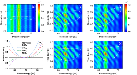
Figure 2. The time-delayed HHG streaking spectra calculated by the EQRS model with five different XUV spectral phases: (a) TL, (b) GDD1, (c) GDD2, (d) TOD1, and (e) TOD2. (f) The spectral phases of the isolated XUV attosecond pulses with the same central photon energy of 71.3 eV and spetral bandwidth of 9 eV.
Download figure:
Standard image High-resolution imageFigures 2(a)–(e) show the simulated HHG streaking spectra of  from equation (11) by using different XUV phases. The spectra are plotted in a photon-energy region overlapped with the spectral region of XUV pulse only. In figure 2(a), the range of time delay is set at about three half-optical cycles (1.33 fs) of the IR laser. One can clearly see the half-optical cycle modulation structure. This structure also appears if other phases are applied (not shown). To see clearly the change of the modulated spectra, we set the range of time delay as about one half-optical cycle in figures 2(b)–(e). The dashed (white) lines are the contour lines in which the intensity is 40% of the peak intensity for each photon energy. With the help of these lines, we can visually identify the change of the streaking spectra by varying the spectral phase of the XUV pulse, especially the change of time delay for the peak intensity. Since the HHG streaking spectra are sensitive to the XUV phase, it would be possible to precisely retrieve the XUV phase from such spectra.
Staring from HHG streaking spectra in figure 2, we reconstruct the spectral phase of XUV pulse as in the following. We take figure 2(b) for example. First, for a specific frequency ωi
, i.e. photon energy of 71.3 eV, the original data describing the variation of spectral intensity with the time delay is shown in figure 3(a). Here the step in time delay is assumed as 10 a.s. To obtain the accurate peak position in each oscillation cycle, we increase the number points in time delay and get the spectral intensity by the Newton interpolation. The results are shown in dashed (red) line in figure 3(a). We then use these peak positions to construct a smooth envelope by using the least square fitting method as shown by a dotted (blue) line in figure 3(a). The peak of this envelope determines the value of time delay when the modulated spectra reach the maximum at a given photon energy. This forms one point labeled as 'cross' in the solid (black) line in figure 3(b). This procedure can be repeated for other photon energies to fully obtain the data of  (solid black line). Then we smooth these data (dashed red line) to get rid of some peculiar points due to errors in the fitting procedure for the smooth envelope of HHG modulation intensity. Finally, according to equation (29), the spectral phase can be reconstructed from HHG streaking spectra.

Figure 3. (a) The time-delayed HHG streaking spectrum at the photon energy of 71.3 eV, including original data (solid black line) from figure 2(b), interpolated curve (dashed red line), and fitted envelope (dotted blue line). (b) The time delay for the peak of modulation spectrum envelope as a function of the photon energy obtained by the fitted envelope in (a) (solid black line) and the time delay versus the photon energy after smoothing (dashed red line).
Download figure:
Standard image High-resolution imageFor the three selected HHG streaking spectra shown in figures 2(a), (b), and (d), the reconstructed XUV spectral phases are shown in the left column of figure 4. Clearly the retrieved phases are very accurate compared to the 'input' data, some discrepancies appear near the wings where the spectral amplitudes are already small. To further check the accuracy of the retrieval algorithm, we show the reconstructed temporal profiles of XUV pulses on the right column of figure 4. The spectral amplitudes of XUV pulse are assumed known as Gaussian. One can see that the retrieved XUV pulses overlap almost perfectly with the 'input' ones. The error in the FWHM duration of XUV pulse is only a few attoseconds, and the biggest relative error is less than 3%.

Figure 4. Characterization of isolated XUV pulses centered at 71.3 eV with a bandwidth of 9 eV. Comparison of the retrieved (solid black lines) and 'input' (dashed red lines) spectral phases (a)–(c) and temporal profiles (d)–(f) of XUV pulses. Note that the spectral amplitudes are assumed the same for the three XUV pulses. The dressing IR laser has wavelength of 800 nm, duration of 5 fs, and peak intensity of 2.5 × 10¹⁴ W cm−2.
Download figure:
Standard image High-resolution image3.3. Retrieval of IAPs in the SXR region
We check whether our retrieval algorithm can be employed to reconstruct the spectral phase of IAPs with a broad bandwidth in the SXR region. We choose three attosecond pulses with the central photon energy of 300 eV and the spectral FWHM bandwidth of 45 eV, which would result in a 40 as pulse under the transform-limited condition. The peak intensity of the SXR pulse is fixed at 5.0 × 10¹¹ W cm−2, and three different input spectral phases are shown as dashed (red) lines in figures 5(d)–(f). The distribution of spectral intensity is also shown as a dotted (blue) line in figure 5(d). We employ a MIR laser pulse with pulse duration of 20 fs, wavelength of 1600 nm, peak intensity of 5.0 × 10¹⁴ W cm−2, and CEP of zero. The simulated HHG streaking spectra by the MIR laser pulse and the time-delayed isolated SXR pulses are plotted in figures 5(a)–(c). We cannot visually observe the interference fringes in these spectra because the optical period of the SXR pulse is much smaller than the time-delay range. One can see that the prominent modulation structures are dramatically changed by varying the SXR spectral phase. Using the same procedure as discussed in section 3.2, we reconstruct the spectral phases shown as solid (black) lines in figures 5(d)–(f). And the retrieved temporal profiles of isolated SXR pulses are plotted in figures 5(g)–(i). The retrieved pulse durations are 480.1 as, 70.8 as, and 41.4 as, compared with the 'input' ones of 487.4 as, 70.3 as, and 41.7 as, respectively. The biggest relative error in the duration of SXR pulse is less than 1.5%.
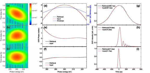
Figure 5. Characterization of three isolated SXR pulses centered at 300 eV with a bandwidth of 45 eV. (a)–(c) The HHG streaking spectra simulated by the EQRS model. The retrieved spectral phases (d)–(f), temporal intensity profiles and FWHM durations (g)–(i) of SXR pulses are compared with the 'input' ones. Note that the spectral intensities of the three SXR pulses are assumed the same (dotted blue line) in (d). See text for the parameters of dressing MIR laser.
Download figure:
Standard image High-resolution imageIn the examples above, the assumed form of the phase over a broad spectral region is relatively simple. Can the spectral phase be accurately retrieved if it has a more complicated behavior in a more broader SXR region. We consider a chirped SXR pulse with the central photon energy of 280 eV and the spectral bandwidth of 90 eV. Its spectral phase is plotted as a dashed (red) curve in figure 6(b). We employ the same MIR laser pulse, and keep the same peak intensity of SXR pulse as those in figure 5. With the simulated HHG streaking spectra in figure 6(a), we obtain the retrieved spectral phase of SXR pulse shown as a solid (black) line in figure 6(b). It shows some derivations with the 'input' phase. The reconstructed temporal profile of SXR pulse, as shown in figure 6(c), presents a good overlap with the 'input' one. The retrieved pulse duration is 27.7 as while the 'input' value is 24.3 a.s. This example verifies that our method is capable of accurately retrieving ultrashort isolated SXR pulses with complicated phase.

Figure 6. Characterization of an isolated SXR pulse centered at 280 eV with a broad bandwidth of 90 eV. (a) The HHG streaking spectra simulated by EQRS model. (b) The spectral phase and (c) temporal intensity profile of the SXR pulse: retrieved (solid black line) versus 'input' (dotted red line) values.
Download figure:
Standard image High-resolution image3.4. Robustness of the phase retrieval method
In the above numerical investigations, we assume that the IR (or MIR) laser pulse can produce the high harmonic spectrum, whose spectral region can well overlap with that of the XUV (or SXR) pulse. However, the IR (or MIR) laser pulse cannot be known exactly in the experiment. We next investigate how the change of IR (or MIR) laser can influence the accuracy of our retrieval method. We take an example of the isolated SXR pulse in figures 5(e) and (h), and the parameters of the MIR laser are kept the same except for the peak intensity. For three peak intensities, the simulated HHG spectra by the MIR laser pulse alone are varied in both the spectral structure and spectral intensity, see figure 7(d). As shown in figures 7(a)–(c), with the increase of the MIR intensity, the modulated HHG spectra maintain their shapes, but become much brighter compared to the background signals. This does not affect the accuracy of the retrieved spectral phase. As shown in figure 7(e), three retrieved spectral phases at different MIR intensities are all in good agreement with the 'input' value. The agreement of retrieved temporal profiles of SXR pulses with the 'input' one in figure 7(f) further shows that the accuracy of retrieval method does not change by varying the peak intensity of the MIR laser. We have also checked the CEP effect of IR (or MIR) laser, which contributes to a linear term in the spectral phase, i.e. αi differs from τi in equation (27) by a constant, leading to an overall time shift of XUV (or SXR) pulse only. Thus the accuracy of retrieval method is not changed by changing the CEP of the IR (or MIR) laser.

Figure 7. The HHG streaking spectra simulated by varying the peak intensity of the dressing MIR laser: (a) 4.5I0, (b) 5.0I0, and (c) 5.5I0, where I0 = 1 × 10¹⁴ W cm−2. (d) The single-atom HHG spectra calculated by the single-color MIR laser pulse. The retrieved spectral phases (e) and temporal intensity profiles (f) of SXR pulses are compared with the 'input' ones (dashed-dotted green lines).
Download figure:
Standard image High-resolution imageWe next check how the intensity of the IAP pulse affects the accuracy of our retrieval method. For the examples of the isolated SXR pulse shown in figures 5(d) and (g), all parameters are kept the same except for the peak intensity of the IAP. We show the simulated HHG spectra in figures 8(a)–(c) by varying the intensity of the SXR pulse by an order of magnitude. The retrieved spectral phases and the temporal pulse profiles are shown in figures 8(d) and (e), respectively. One can see the relative error in the retrieved duration of the SXR pulse is less than 4%. Note that with the decrease of intensity of the IAP, the modulation structure in the HHG streaking spectra becomes faint which might not be desirable in such experiments.

Figure 8. The HHG streaking spectra simulated by varying the peak intensity of the SXR pulse: (a) 1 × 10¹¹ W cm−2, (b) 5 × 10¹⁰ W cm−2, and (c) 1 × 10¹⁰ W cm−2. The retrieved spectral phases (e) and temporal intensity profiles (f) of SXR pulses are compared with the 'input' ones (dashed-dotted green lines).
Download figure:
Standard image High-resolution imageWe also check another factor of the time-delay step for obtaining the 'input' HHG streaking spectra. In the experiment, this is varied due to the capability of precisely controlling the two-color laser beams. We use the same SXR pulse and MIR laser as those in figure 7, and the peak intensity of MIR laser is set at 5.0 × 10¹⁴ W cm−2. The pulse duration of the MIR laser is changed to 10 fs. The central photon energy of the SXR pulse is 300 eV, and its spectral bandwidth is 45 eV. We set the step of time delay between the SXR pulse and the MIR laser as 20 as, 30 as, 40 as, and 50 as, respectively. These values are all larger than the modulation period of HHG spectra along the time delay, which is close to one optical cycle of the central SXR frequency, i.e. 15 a.s. Thus the resulted streaking spectra in figures 9(a)–(d) show different patterns visually. The retrieved spectral phases of SXR pulse are plotted in figure 9(e). We have checked that the result obtained by the step of 20 as is almost identical with the 'input' one, and it can be considered as a reference here. One can see that the retrieved phase changes a little bit randomly by increasing the step of time delay. The reconstructed temporal profiles of SXR pulses are plotted in figure 9(f). The peak of retrieved pulse is slightly shifted with the time-delay step, but its shape remains and the retrieved duration still has the high accuracy. From the duration values labeled in the figure, the biggest relative error in the SXR pulse duration is about 4%. So the accuracy of retrieval maintains if the step of time delay in measuring the HHG streaking spectra is much bigger than the spectra modulation period. In a real experiment, the time delay cannot be perfectly stabilized and a jitter with the scale of few tens attoseconds should be considered. We have checked that retrieved results are accurate and stable even a random and reasonable shift in time delay is added for simulating the HHG streaking spectra.

Figure 9. The modulated HHG spectra obtained by using four different time-delay steps: (a) 20 as, (b) 30 as, (c) 40 as, and (d) 50 a.s. The retrieved spectral phases (e) and temporal profiles (f) of SXR pulses are shown.
Download figure:
Standard image High-resolution image3.5. Retrieval of the XUV pulse from TDSE-based HHG streaking spectra
The HHG streaking spectra used for retrieving the spectral phase of XUV (or SXR) pulse so far are all simulated by using the EQRS model. Here we test if the spectral phase can be accurately reconstructed from the 'experimental' spectra, which is taken to be the HHG streaking spectra obtained by numerically solving the TDSE [57]. The TDSE solution is a three dimensional simulation obtained under the dipole and the single-active electron approximations with the effective potential taken from [60]. Based on the TDSE simulations, we define that  is the dipole acceleration under the IR laser and the time-delayed XUV pulse,
  and
and  are the dipole accelerations solely caused by the XUV pulse at a time delay τ and by the IR pulse, respectively. We then use these quantities in the frequency domain, and let

where n is an integer and it meets the condition of  with the IR period TIR, and the IR total pulse duration Ttotal.
  gives the dipole response when the IR laser and the XUV pulse are overlapped while
  is the response when the two pulses are well separated in time. Both the spectra from the two terms can be directly measured in the experiment at different time delays between the IR laser and the XUV pulse. Thus, through equation (31), modulation of the HHG streaking spectra with time delay becomes clearly visible and is consistent with that simulated by the EQRS model. We take the example of retrieving a narrow-bandwidth XUV pulse. The parameters of IR laser and XUV pulse are the same as those in section 3.2. For two different spectral phases, the TDSE-based modulation spectra are modified, see figures 10(a) and (b). Using our phase retrieval method, the spectral phases can be well reconstructed, see figures 10(c) and (d). The retrieved temporal profiles of the XUV pulse also show good agreement with the 'input' ones, see figures 10(e) and (f). The retrieved pulse durations of 215.9 as and 445.9 as can be well compared with the 'input' ones of 200.5 as and 486.3 as, respectively. The biggest relative error in the retrieved pulse duration is about 8% in these two cases.

Figure 10. Characterization of isolated XUV pulses by using the HHG streaking spectra ((a) and (b)) simulated with the TDSE method. The retrieved spectral phases ((c) and (d)) and temporal intensity profiles ((e) and (f)) are compared with the 'input' ones. The XUV pulses are centered at 71.3 eV with the bandwidth of 9 eV.
Download figure:
Standard image High-resolution image
4. Summary
In summary, we established an all-optical method for the retrieval of the spectral phase of IAPs using the modulated HHG streaking spectra generated by the combination of a linearly polarized XUV (or SXR) pulse with a time-delayed intense IR (or MIR) laser. Deriving from the SFA and the EQRS model, at each photon energy, the derivative of the IAP spectral phase is directly related to the time delay, at which the peak of the modulated HHG spectra occurs. Different from most retrieval algorithms used for attosecond photoelectron streaking experiments, our method does not rely on the iterative procedure, thus errors in the retrieved results are introduced only by the experimental measurements and the model itself, but not by the convergence of the iterations. Note that, compared to the earlier retrieval method in [55], a significant advance has been made in the present version such that the spectral phase of any form can be directly extracted from the HHG spectra, even for the irregularly behaved phase. We showed that our method can well retrieve the spectral phases (or the temporal intensity profiles) for both isolated XUV and SXR pulses, which have a narrow bandwidth in the XUV and a broad bandwidth in the SXRs, respectively. Meanwhile, the robustness of the retrieval method was examined by either changing the peak intensity of the MIR laser or by varying the step of time delay. Finally, we also checked that the isolated XUV pulses can be well characterized by using the HHG streaking spectra simulated with the TDSE method.
In the present retrieval method, only the spectral phase of IAP can be reconstructed from the HHG streaking spectra. As demonstrated in the FROG-CRAB method with the attosecond streaking spectra [31, 36, 43], the spectral amplitude of IAP and the dressing IR laser can also be reconstructed. How to achieve these goals will be investigated after improving our retrieval method. In this work, we only use the single atom HHG streaking spectra simulated by the EQRS or the TDSE as 'experimental' data. As one knows, the macroscopic propagation effects are involved in the generation of HHG streaking spectra [61–63]. How accurate our retrieval method is will be examined under a variety of phase-matching conditions by further incorporating the EQRS model with the theory of macroscopic propagation. Furthermore, the spectral phases in the current examples have been assumed relatively smooth. If the IAP spectrum contains 'Cooper'-minimum like structure, its spectral phase would have a big jump around the minimum and its temporal profile will be split [64–66]. How to deal with such IAPs should also be considered in the future.
Acknowledgments
This work was supported by Natural Science Foundation of China (NSFC) (12274230, 91950102, 11834004, 12204238), National Science Foundation of Jiangsu Province (BK20220925), and Funding of Nanjing University of Science and Technology (NJUST) (TSXK2022D005); C D L was supported by Chemical Sciences, Geosciences and Biosciences Division, Office of Basic Energy Sciences, Office of Science, U S Department of Energy (DE-FG02-86ER13491).
Data availability statement
All data that support the findings of this study are included within the article (and any supplementary files).
Appendix: Derivation of some formulas in section 2.2
Appendix. Derivation of the XUV temporal expression in equation (18)
By taking the Fourier transform of the i-th electric field  in the frequency domain in equation (14), its temporal expression can be written as
We define

and the field expression of  can be simplified as

The above equation can be calculated as
The definite integral of  is used.
Therefore, the complex expression of  is
is

If we only keep the real part,  can be expressed as

Appendix. Derivation of equation (24)
The equation (23) is expressed as

Its right hand side can be written as

where

By substituting the explicit form of  in equation (18) into the above equation, one obtains

We define

and then we have
Then the common integral term in the above equation is
where  =
=  or
or  . The integral with the same form as equation (44) also appears in equation (48), below which the approximated approach to get its value is given in equation (54). When
  , the exponential term in equation (44) is approximately equal to zero since
  . Therefore, equation (43) can be simplified as

In equation (45), only when  ,
,  has a considerable value in the summation in equation (39), thus equation (38) can be reduced as

Appendix. Derivation of equation (25)
Let
Using defined constants in equation (42), we have
In the following, we calculate the two integrals in the above equation separately. First we expand the electric field  by Taylor series at the time
  as
as

The  is the nth derivative of the electric field at time
  . We keep the first three terms in the expansion, and substitute the expansion form of
  into the second integral of equation (48) as
Using the definite integral of the Gamma function in the following

the second integral becomes

Since the FWHM duration of the i-th XUV pulse  is shorter than the optical cycle of the IR field, the IR electric field can be considered slowly varying, meaning that
  . Thus we have

We use the same approach to calculate the first integral of equation (48) as
We expand the function of  as
as
Thus we have
In the above equation,  . By considering the integral of the Gamma function, we get

where n + m is set as even number. Using the same argument for the second order derivative of  previously,
  with
with  (even number), so the above equation equals to zero. We define

and we have the integral in the first term of equation (54) as
Thus we have

Since  , the above equation is approximately equal to zero. The first integral term in equation (48) can thus be ignored. Therefore, equation (48) can be written as

Thus equation (24) is expressed as
