


Abstract
We analyse the transport of diffusive particles that switch between mobile and immobile states with finite rates. We focus on the effect of advection on the density functions and mean squared displacements (MSDs). At relevant intermediate time scales we find strong anomalous diffusion with cubic scaling in time of the MSD for high Péclet numbers. The cubic scaling exists for short and long mean residence times in the immobile state  . For long
  the plateau in the MSD at intermediate times, previously found in the absence of advection, also exists for high Péclet numbers. Initially immobile tracers are subject to the newly observed regime of advection induced subdiffusion for short immobilisations and high Péclet numbers. In the long-time limit the effective advection velocity is reduced compared to advection in the mobile phase. In contrast, the MSD is enhanced by advection. We explore physical mechanisms behind the emerging non-Gaussian density functions and the features of the MSD.
Export citation and abstract BibTeX RIS

Original content from this work may be used under the terms of the Creative Commons Attribution 4.0 license. Any further distribution of this work must maintain attribution to the author(s) and the title of the work, journal citation and DOI.
1. Introduction
One of the simplest equations to describe the transport of tracers in subsurface aquifers (water-bearing layers or permeable rock or sediment) is the advection–diffusion equation [1, 2]

where  denotes the probability density function of a tracer particle, v the constant advection velocity, and D the diffusion constant. The initial condition is
  , corresponding to a 'point injection' in geoscience. The probability density function encoded by equation (1) with initial condition
  is given by the Gaussian

with similarity variable x − vt, where the first moment  and the mean squared displacement (MSD)
 ![$\langle [x(t)-\langle x(t)\rangle]^2 \rangle = 2Dt$](https://content.cld.iop.org/journals/1367-2630/25/6/063009/revision2/njpacd950ieqn7.gif) are linear at all times. The latter does not depend on v. The alternatively used mobile–immobile model (MIM) is a more elaborate model that takes pores into account, where a tracer can remain immobile for an exponentially random duration [3–5]. This linear first order mass transfer is often used to model sorbing solutes, as well [6–8]. In an MIM the concentration is split into a mobile density
are linear at all times. The latter does not depend on v. The alternatively used mobile–immobile model (MIM) is a more elaborate model that takes pores into account, where a tracer can remain immobile for an exponentially random duration [3–5]. This linear first order mass transfer is often used to model sorbing solutes, as well [6–8]. In an MIM the concentration is split into a mobile density  and an immobile density
  . In the mobile state tracers are subject to advection and diffusion in the same way as in the advection–diffusion equation (1). MIMs have been used extensively in geophysical systems [3, 4, 8–18]. Apart from geophysical applications, we mention two other applications, where motion interrupted by transient immobilisations has been studied. The first application pose biological systems, such as potassium channels in the membrane of living cells [19] and transcription factors [20]. Many systems such as tau proteins [21, 22], synaptic vesicles [23], complexes at the endoplasmic reticulum [24], the drug molecule doxorubicin in silica nanoslits [25] and DNA binding proteins [26–35] may be described in terms of an MIM, in which the residence times in the immobile state are distributed exponentially
5
. The corresponding experiments were conducted in flow cells [26, 32–35] or occur in live biological cells [27–30]. In such cellular systems advection may arise due to the action of molecular motors causing streaming in the cytoplasm [36]. Further examples of systems with advection, where in addition immobilisations occur, include DNA molecules in microfluidic setups and bio sensors [37, 38]. The second application, featuring transient immobilisations concerns charge carriers in semiconductors, where a recent focus lies on exciton diffusion in layered perovskites and transition metal dichalcogenides [39–42]. Often, MIMs are not formulated in terms of mean residence times but with a single rate for mass exchange and a solute capacity coefficient that takes different volumes of the mobile and immobile volume into account [3, 7, 11, 12, 43]. The moments for mobile, immobile and total density of the MIM have been calculated for various initial conditions while including effects of advection and diffusion [6, 7, 13]. We here focus on the densities and MSDs at relevant intermediate time scales and unveil interesting new properties in the transport dynamics. In the short time limit initially mobile tracers behave like free Brownian tracers (2) with an MSD
. In the mobile state tracers are subject to advection and diffusion in the same way as in the advection–diffusion equation (1). MIMs have been used extensively in geophysical systems [3, 4, 8–18]. Apart from geophysical applications, we mention two other applications, where motion interrupted by transient immobilisations has been studied. The first application pose biological systems, such as potassium channels in the membrane of living cells [19] and transcription factors [20]. Many systems such as tau proteins [21, 22], synaptic vesicles [23], complexes at the endoplasmic reticulum [24], the drug molecule doxorubicin in silica nanoslits [25] and DNA binding proteins [26–35] may be described in terms of an MIM, in which the residence times in the immobile state are distributed exponentially
5
. The corresponding experiments were conducted in flow cells [26, 32–35] or occur in live biological cells [27–30]. In such cellular systems advection may arise due to the action of molecular motors causing streaming in the cytoplasm [36]. Further examples of systems with advection, where in addition immobilisations occur, include DNA molecules in microfluidic setups and bio sensors [37, 38]. The second application, featuring transient immobilisations concerns charge carriers in semiconductors, where a recent focus lies on exciton diffusion in layered perovskites and transition metal dichalcogenides [39–42]. Often, MIMs are not formulated in terms of mean residence times but with a single rate for mass exchange and a solute capacity coefficient that takes different volumes of the mobile and immobile volume into account [3, 7, 11, 12, 43]. The moments for mobile, immobile and total density of the MIM have been calculated for various initial conditions while including effects of advection and diffusion [6, 7, 13]. We here focus on the densities and MSDs at relevant intermediate time scales and unveil interesting new properties in the transport dynamics. In the short time limit initially mobile tracers behave like free Brownian tracers (2) with an MSD  . At long times the MSD is linear, with the effective diffusivity
  containing a term proportional to v2, that can yield
  [7, 13]. This is in contrast to the solution (2) of the advection-dispersion equation (1), in which the MSD does not depend on v. Below we provide a physical explanation for how this enhanced effective diffusion coefficient is brought about. Another model often used to describe the motion of tracers with immobile periods is the continuous time random walk (CTRW) [39, 44, 45], for which it was shown that exponential tails emerge in the position density [46] when a drift is present [13, 18, 47–50]. CTRWs have also been analysed for systems with two states, characterised by two waiting time distributions, such that a specific distribution is chosen alternatingly or randomly [51, 52]. A similar approach to modelling motion interrupted by transient immobilisations was studied in [53]. In the present work we consider a MIM in the formulation with mean mobile residence time
  and mean immobile residence time
  similar to our previous work [54] in the absence of a drift. In [54], the mean immobile residence time
  and mean mobile residence time
  are well separated,
  , corresponding to the one-dimensional motion of tau proteins without advection. At intermediate times
  a Laplace distribution of positions
  with fixed variance was shown to emerge whose prefactor depends on the initial condition, and the MSD of initially mobile tracers displayed a plateau at intermediate times. The main goal of the present work is to analyse how the Laplace distribution and the plateau in the MSD change when advection is added. The transition from the Brownian MSD 2 Dt at short times to
  implies a crossover regime, in which the MSD grows faster than linear given our finding
  . In fact, we find a sustained superdiffusive regime with a cubic anomalous diffusion exponent in the MSD at relevant intermediate time scales. For low advection velocities we recover the model from [54]. Therefore, to highlight new features, we focus on high Péclet numbers
  . An application of the MIM with a high Péclet number may occur for sufficiently long times in subsurface aquifers, in the hyporheic zone or in microfluidic setups. A specific example is the motion of biomolecules in bio sensors, as schematically depicted in figure 1. The biomolecules are inserted into a flow cell and bind to the surface reversibly [38]. The surface is coated with receptors that specifically bind to the molecule of interest. Only the bound molecules can be detected using e.g. surface plasmon resonance [38]. In our model we assume the detector to be completely covered with receptors and consider concentrations well below saturation.

Figure 1. Schematic of a biosensor with flow. A tracer is inserted into the flow cell, where it is subject to advection with velocity v and Brownian diffusion with diffusivity D in the mobile state. With the rate  it binds to receptors on the surface and immobilises. It unbinds with rate
  and continues in the mobile state.
Download figure:
Standard image High-resolution imageIn the next section we introduce the model equations and show two ways to solve the model. The direct way using Fourier–Laplace transform yields the densities in Laplace space and exact expressions for the MSD. Additionally, we show how to solve the advection-MIM using a subordination approach, that produces a physical explanation for the additional term in  due to the variance of times the tracers spend in the mobile state. As mentioned in the following, we consider strong advection and obtain asymptotic expressions for the density and the MSD in the presence of a clear time scale separation, i.e.
  or
or  . For clarity we focus on the detailed behaviour of the MSD of the total density, while the results for the immobile and mobile fractions are summarised in the appendix. The dimensionless form of the model depends on the ratio
  and the Péclet number only. We use these variables in a phase diagram to analyse the anomalous diffusion in the full parameter space including small Péclet numbers. Specifically, in section 2, we formulate and solve our model. In section 3 we consider tracers that are initially mobile and obtain asymptotic expressions of the density functions and MSDs. Special focus is put on finding the parameter regimes where non-Gaussian displacement distributions and anomalous scaling of the MSD emerge. In section 4 we repeat the same analysis for initially immobile tracers. Finally, we summarise and conclude in section 5. The appendix provides details on the calculations and additional figures of the MSDs.
2. Formulation of the model
We employ the MIM with mean mobile residence time  and mean immobile residence time
  in an (effectively) one-dimensional setting with position variable x,
where  and
and  denote the line densities of mobile and immobile tracers, respectively. Advection with velocity v and dispersion with diffusion constant D is exclusively affecting the mobile density. A single tracer switches between the mobile state and immobile state following a two state continuous time Markov process, i.e. it follows a Poissonian switching. The realisation (3) of the MIM corresponds to the model used in [54] with the residence time distribution in the mobile state
  . We add a drift in the mobile state here and will show that this has significant consequences. Splitting the total density
  has the advantage that not always
  is measured in experiments. In a biophysics sensor as sketched in [38], solely the immobile tracers can be measured. In contrast, it is often the mobile density that is measured in geological experiments [12, 18]. In both cases it is thus essential to model the two densities separately. Step or delta injection into the mobile domain is common in geological experiments [10, 12, 55–57]. Our model (3) is very similar to the MIMs used in geoscience, with the difference that there usually the capacity coefficients and porosity, among others, are used instead of the mean residence times [6, 7, 13]. We consider the initial condition
  and
and  where
where  denotes the Dirac-δ distribution. The factors
  and
and  denote the fractions of initially mobile and immobile tracers with
  , which effects the normalisation of the total density,
  . This corresponds to a single-particle picture with no interactions between the tracers, as is the case in model (3). In this work we consider the cases when all tracers are either initially mobile (
 ) or when all tracers are immobile (
 ). We briefly discuss an equilibrium fraction of initially mobile tracers in appendix
2.1. Solution in Laplace space
Fourier–Laplace transform  of the model equations (3) allows solving for the densities, as shown in appendix

as well as (see equation (A.4))
with ![$\phi(s) = s[1+\tau_\mathrm{im}\tau_\mathrm{m}^{-1}/(1+s\tau_\mathrm{im})]$](https://content.cld.iop.org/journals/1367-2630/25/6/063009/revision2/njpacd950ieqn46.gif) . The fraction
. The fraction  of free and the fraction
  of immobile tracers are a function of time and the expressions are given in equation (A.8) in appendix
  . In the long-time limit, the equilibrium fraction
  of all tracers are mobile. We calculate the pth moment (
 ) using

where j stands for  ,
,  , or
, or  [54]. To shorten the notation, we use
  in the remainder of this work. The lengthy exact expressions for the MSD are given in appendix
  is related to the second moment
  in the advection-free setting with the second Einstein relation [58]

This relation becomes obvious when we look at the moments in appendix  was discussed in [54] in detail, we focus on the MSD here.
2.2. Subordination approach
The concept of subordination was originally introduced by Bochner [59] and refers to a process ![$X[\tau(t)]$](https://content.cld.iop.org/journals/1367-2630/25/6/063009/revision2/njpacd950ieqn59.gif) with the operational time τ (in many random walk contexts the number of jumps [44]), which has random non-negative increments. For the operational time τ the propagator is known, in our case the Gaussian
with the operational time τ (in many random walk contexts the number of jumps [44]), which has random non-negative increments. For the operational time τ the propagator is known, in our case the Gaussian  (2). Then, the subordinator relates the stochastic increases of τ to the process (laboratory) time t measured in the real-world observation. In our model the stochasticity comes from the immobilisations, where t increases even while τ is stalling. Assume that we know of a single tracer when it is mobile and when it is immobile. Let i(t) be the index function that is unity if the tracer is mobile at time t and zero otherwise, as shown in figure 2. The index function follows a two-state continuous-time Markov process (telegraph process) with mean residence time
  in state 1 and mean residence time
  in state 0. As described in [60–62] (compare also [63]), this allows us to write a Langevin equation of the form


with the operational time τ, that is a random quantity, and zero-mean white Gaussian noise with correlation  . Figure 2 shows two samples of
  for
for  and
and  in the upper panel. The lower panel shows the corresponding trajectory x(t) for
  and v = 2. The propagator with this new variable τ is given by
  (2). In appendix
  and its moments using Laplace transforms. In figure 3 we show the numerical Laplace inversion of
  (D.12) for three values of t and the parameters
  and
and  . In order to verify our approach, we compare the Laplace inversion to the solution
  obtained in [23], that is presented in appendix
  converges to a Gaussian with mean
  and variance
  , as shown by the dashed line following a Gaussian with that mean and variance (see the moments above). With
  we can eliminate
  and find using the well established method of subordination [60–65]

where  denotes the propagator (18) in the mobile phase. Expression (11) can be written in the form (6) of
  by inserting the subordinator
  in Laplace space. In appendix
  and
and  in a similar way.
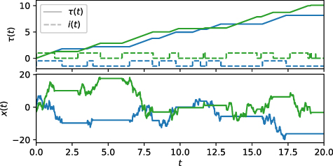
Figure 2. Upper panel: two realisations of  for
for  and
and  . The process time τ increases with t, whenever the tracer is mobile and the index function i(t) is unity. The realisation corresponding to the shown indicator trace i(t) is rendered in the same colour. For clarity, the blue line corresponding to i(t) is shifted in the y direction by
  . Lower panel: corresponding trajectories x(t) for
  and v = 2, which take on constant values whenever
  .
.
Download figure:
Standard image High-resolution image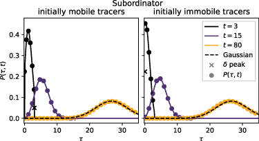
Figure 3. Comparison of  , equation (D.1) (coloured discs) with the Laplace inversion of
  (D.12) (solid lines) and a Gaussian with mean
  and variance
  (dashed line). The crosses mark the amplitudes of the delta peaks at x = vt and the origin for initially mobile and immobile tracers, respectively. Parameters:
  and
and  .
.
Download figure:
Standard image High-resolution image2.3. Dimensionless form
Our model (3) has the four parameters  ,
,  and D. We now show that in a dimensionless form the model depends only on two free parameters, which significantly reduces the space of parameters we need to consider in order to obtain a full picture of the model. Moreover, this highlights the conceptual simplicity of the model. To this end, we define the new dimensionless variables
  and
and  . In these variables the model (3) turns into the set of equations

which only depends on the immobilisation ratio  and the Péclet number
  . The typical length scale for the latter is given by
  . The factor
  in the Péclet number is introduced for convenience. To see this, we note that from the Péclet number we obtain the advection time scale
  , which naturally arises from the solution to the advection-diffusion equation (2) as follows. The typical distance travelled due to advection and dispersion is given by
  and
and  , respectively. Comparing these distances gives the time scale
  , after which displacements due to advection dominate over diffusive displacements.
2.4. Short-time behaviour
In the mobile phase tracers are being propagated with the Gaussian (2). As described above the displacements are diffusion dominated for  . This means that the tracers follow the same density as in the case without advection, which is described in detail in [54]. To emphasise the effects of advection we therefore choose
  . This defines the short-time limit
  .
.
2.5. Long-time asymptote
The densities of the total, mobile and immobile density are, up to a factor, the same in the long-time limit  [5]. In absence of advection, the effective long-time diffusivity is given by
  for
for  [54]. Tracers disperse slower compared to the model of simple diffusion advection without immobilisation (1) with diffusivity D. We now obtain
  by analysing the asymptotic behaviour
  of the expressions for the MSD. The exact expressions for the first and second moments are stated in appendix

where ∼ denotes asymptotic equivalence with an additional spread  compared to the case without advection. Remarkably, the asymptotic dispersion with the new effective diffusion coefficient

can hence even be higher than the diffusivity D in the mobile state and overcompensate the slow-down of the spread due to immobile durations. In appendix  . As shown in figure H1, the increase of
  is highest, when
  and
and  are of the same order. A physical intuition for the additional spread due to advection arises from the special case D = 0, for which
  with the mobile duration τ. Due to the stochastic switching between the mobile and immobile state, an ensemble of tracers will have a distribution of mobile durations τ (the density
  in section 2.2), and hence the positions will have a finite spread. This additional spread was derived before [6, 13], albeit without a more detailed physical justification. The anomalous transport regime at intermediate times that necessarily has to exist to effect the crossover between the two normal-diffusive regimes, and the important physical consequences will not be explained
6
. We explore the physical mechanism behind the additional dispersion due to advection in the long-time asymptote (14) of the MSD. We start by discretising the advection-diffusion process into discrete steps
in section 2.2), and hence the positions will have a finite spread. This additional spread was derived before [6, 13], albeit without a more detailed physical justification. The anomalous transport regime at intermediate times that necessarily has to exist to effect the crossover between the two normal-diffusive regimes, and the important physical consequences will not be explained
6
. We explore the physical mechanism behind the additional dispersion due to advection in the long-time asymptote (14) of the MSD. We start by discretising the advection-diffusion process into discrete steps  that are normally distributed
  , where each step takes a small duration
  . After n steps the tracer position is given by
  . In the long-time limit the number of steps n follows a Gaussian
  , as described in section 2.2
7
. The number of steps n is independent of the steps
, as described in section 2.2
7
. The number of steps n is independent of the steps  . With the expectation value
  and the variance
  we obtain the expression [66]

for  . Equation (16) demonstrates that in the case of diffusion without advection only the mean mobile duration affects the MSD. In contrast, advection couples to the mean in the first moment and to the variance of the duration that the tracers spend in the mobile state in the MSD (14).
All time scales in the model are finite, and therefore the density converges to the Gaussian

in the long-time limit with the effective diffusion coefficient  (equation (15)) and the effective advection velocity
  (see appendix B.1). In the next two sections we analyse the densities and MSDs for the specific choice of initially mobile and immobile tracers, respectively.
3. Initially mobile tracers
In this section we assume all tracers to be initially mobile. This situation corresponds to many experimental realisations, when tracers are introduced into the system, such that they have not had a chance to immobilise. We consider the following four aspects. In section 3.1 we assume  , which corresponds to a high Péclet number and long immobilisations to emphasise the effect of advection compared to [54]. In section 3.2 we consider the density for short immobilisations and high Péclet numbers,
  . The third section 3.3 is concerned with the MSD for which we obtain expressions for superdiffusion at intermediate time scales arising due to advection. In the final subsection appendix I.1 we analyse for which parameters the uncovered superdiffusive regime exists and how it is competing with the plateau regime in the MSD found in [54] for long immobilisations in the advection-free regime.
3.1. Densities for long immobilisations
Initially mobile tracers that have not yet immobilised follow a Gaussian distribution corresponding to free Brownian motion without advection for  . At short times
  advection is negligible in the Gaussian propagator and the density is the same Gaussian with mean
  close to zero and variance 2 Dt. At intermediate times
  advection becomes relevant, and the mobile density takes on the Gaussian form
with  corresponding to a scaled solution of the simple diffusion advection equation (1)
8
. The Gaussian (18) is shown as a dashed red line in the first two panels of figure 4, in which a stacked position histogram from simulations is shown in which the colours denote the number of immobilisation events
corresponding to a scaled solution of the simple diffusion advection equation (1)
8
. The Gaussian (18) is shown as a dashed red line in the first two panels of figure 4, in which a stacked position histogram from simulations is shown in which the colours denote the number of immobilisation events  . The solid lines are obtained from Laplace inversion of
  ,
,  , and
, and  from equations (5) and (6). We use the parameters
  ,
,  ,
,  and v = 100. These parameters are specifically chosen to be able to resolve the multiple time regimes. In the short to intermediate time regime
  , where t can be shorter or longer than τv
, the immobile density consists of tracers that immobilised at most once. In equation (F.2) in appendix
, where t can be shorter or longer than τv
, the immobile density consists of tracers that immobilised at most once. In equation (F.2) in appendix
for  . The mass corresponding to (19) is
  , corresponding to 10−3 in the left panel of figure 4. This value is very small and hence the immobile density is not visible in the first panel.

Figure 4. Semi-log stacked position histogram with overlaid Laplace inversions of the mobile and total densities (4) and (6) for initially mobile tracers and long immobilisations  . The bars of the histogram are coloured according to the number of immobilisation events
  . The density of initially mobile tracers has four time regimes for
  . For short to intermediate time scales
  , where t can be smaller or larger than τv
the mobile density follows the Gaussian (2) with variance 2 Dt and mean vt, and the number of immobilisations
, where t can be smaller or larger than τv
the mobile density follows the Gaussian (2) with variance 2 Dt and mean vt, and the number of immobilisations  is zero, as shown by the black area. The blue dashed line shows the asymptote of the immobile density (19) for
  , where t can be smaller or larger than τv
. In that domain the density consists of the same Gaussian and an additional uniform distribution of immobilised tracers shown by the red area in the second panel. For
, where t can be smaller or larger than τv
. In that domain the density consists of the same Gaussian and an additional uniform distribution of immobilised tracers shown by the red area in the second panel. For  almost all tracers immobilised exactly once and follow a Laplace distribution (23) with different scale parameters for the positive and negative x direction. In the long-time limit
  , after many immobilisations the density follows the Gaussian (17) with mean
  and effective diffusion constant
  . See text for details. Parameters:

 v = 100.
Download figure:
Standard image High-resolution imageThe immobile density in figure 4 appears to be uniform at t = 0.1. Indeed, for  the short-time density (19) approaches a uniform distribution. Using the properties of the error function we arrive at the asymptotic uniform distribution

valid for  . This shape can indeed be seen in the second panel of figure 4, for which the immobile density remains almost constant for
  . The approximation (19) is shown as the blue dashed line. In the same panel the Gaussian (18) is shown as the dashed red line. The total density is given by

for  with
with  . The appearance of this regime is new, as compared to the case without advection [54]. A physical picture for the occurrence of the uniform density of immobile tracers is as follows. For
  advective transport dominates over diffusion. Indeed, the typical distance a tracer moved due to advection is given by the mean position vt, while the typical distance travelled due to diffusion is given by the standard deviation
  . The mobile tracers hence move with a narrow Gaussian distribution while a fraction of tracers immobilises with the constant rate
  , which generates the uniform part of the distribution (see figure 4 for t = 0.1).
Now we go to immobilisation dominated intermediate times  . This regime is easy to analyse when starting from the density in Laplace space. We have
  for
for  and find the expression

from  (6), which in time-domain corresponds to

for  . Expression (23) is a normalised distribution with time-independent parameters, that falls off exponentially in the positive and negative x direction with different coefficients. It is shown in the third panel in figure 4 for t = 10 as the grey dashed line. The density falls of quicker in the direction opposite to the advection velocity, as expected. Noteworthily, the Laplace distribution occurs for all values of the Péclet number, i.e. v can take on any value in the asymptote (23).
For long times  , we show the Gaussian (17) in figure 4 as a red dashed line for
  . The Gaussian (17) contains the effective advection
  and the effective diffusivity (15), that we obtained in section 2.5.
3.2. Densities for short immobilisations
Now we turn to the case of short mean immobile residence times,  . For short times
  and intermediate times
  the mobile density follows the same Gaussian (18) as for long immobilisations. This can be seen in figure 5 in the first panel for t = 0.1. From simulations, we obtain position histograms that we colour-code according to the number of immobilisations. Most tracers have not immobilised at this time, as shown by the dominant black area that follows the Gaussian (18). The tracers that did immobilise follow the same asymptote (19) of
  as for long immobilisations, as depicted by the dashed blue line. Beyond
  immobile tracers become mobile again and contribute to the mobile density. This can be seen in figure 5 in the second panel for t = 1 by the red area in the mobile density denoting tracers with a single immobilisation event. In figure 5, the total density appears to have an exponential tail in the opposite direction of the advection velocity for t = 10 and t = 20 in the third and fourth panel, respectively. We now investigate the origin of this phenomenon. For
  , the fraction
  of mobile tracers is trapped for a short period τ drawn from
  . This is shown as the red area in figure 5 denoting a single immobilisation. Hence, these tracers were mobile for a total period of
  . We convolute this with the propagator for advection diffusion. Together with tracers that have not immobilised this gives the total density for
  ,
,

The integral on the right-hand side can be solved and is given by
for  with the complimentary error function
  . In appendix
  , i.e. intermediate Péclet numbers. Approximation (24) is shown in figure 5 as the dashed dark-yellow line and follows the density for x > 70 at t = 10 and matches almost the entire density at t = 20. For
  and
and  expression (24) simplifies to

This tail approximation is only valid close the origin. For this reason it is not normalised. It is shown in figure 5 as the solid grey line. The tail overlaps with expression (24) shown as the dashed dark-yellow line. The second exponent in expression (26) reveals that the slope of the tail does not depend on time. The slope decreases for larger values of  . As described in detail in section 2.5 the long-time asymptote
  of the density follows a Gaussian with an effective advection speed and an effective diffusivity.
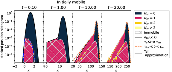
Figure 5. Semi-log stacked position histogram with overlaid Laplace inversions of the densities for initially mobile tracers and short immobilisations  . Particle densities from Laplace inversions of equations (4) to (6) are shown as solid lines with
  . The grey striped area denotes the immobile particles and the colour code denotes the number of immobilisations
  . The short to intermediate time asymptote (19) for
  , where t can be shorter or longer than τv
, is shown as the blue dashed line. The asymptote (24) for intermediate times
, where t can be shorter or longer than τv
, is shown as the blue dashed line. The asymptote (24) for intermediate times  is shown as the orange dotted line and its exponential asymptote (26) as the solid grey line. Parameters: v = 12.5,
  ,
,  and
and  .
.
Download figure:
Standard image High-resolution image3.3. Mean squared displacement
In this section we analyse the MSD of the total density. In appendices E.1.1 and E.1.2 we analyse the MSD of the immobile and mobile density, respectively. We now investigate how advection changes the MSD as compared to the results presented in [54]. Table C1 shows a series of the total, mobile and immobile MSDs for initially mobile and initially immobile tracers for  . In all cases, the leading order term does not depend on v. Therefore, for short times the MSDs are equivalent to the MSD without advection.
In figure 6(a) the MSD for initially mobile tracers is shown for long immobilisations,  , where the solid black line corresponds to the total density's MSD. In panel (b) we show the MSDs for short immobilisations,
  . For comparison, we show the MSD for the case without advection in grey. It can be seen that the corresponding MSDs with and without advection overlap for
  . After a linear short-time behaviour for
  the MSD crosses over to a cubic scaling for
  . Our goal is to quantify the cubic scaling and determine the value of
  . From a series expansion of the exact expression for the MSD (exact expressions for the moments are given in appendix

In figure E2 we compare equation (27) to the full expression of the MSD and find very nice agreement. A cubic scaling of the MSD (27) emerges at intermediate times when the cubic term dominates over the linear term in equation (27). This corresponds to the relation  with
with  . Indeed, the cubic scaling of the total MSD is shown in figure 6(a) in the domain
  . Notably, it occurs also for
  , as shown in figure 6(b). This cubic scaling is new compared to the case without advection. It lies within the domain where we found an advection dominated regime
  in the previous section, in which the density (21) consists of a uniform and a Gaussian distribution with time-dependent weights. In figure E1 we show the MSD and choose such parameters that emphasise that the intermediate cubic scaling can be more than a bare crossover but corresponds to a distinct anomalous regime. We now show that the anomalous diffusion arises from this distribution. First we consider the uniform distribution ranging from zero to vt. It has the first moment
  and the second moment
  with the MSD
  . This is the dominating term of the immobile density's MSD for
  , as shown in figures 6(a) and (b), where the quadratic scaling can be observed. Second we recall the first and second moments of the mobile Gaussian distribution
  and
and  . Now we consider the MSD of the total density by combining the moments with the normalisations
  and
and  for the uniform and Gaussian distribution, respectively. This leads to the same asymptotic MSD (27), as obtained by the series expansion, as the following calculation shows:
The asymptotic expression is identical to what we found from the exact expressions (27). This shows indeed that the uniform distribution and the Gaussian distribution can indeed explain the cubic scaling. The cubic scaling of the MSD emerges for  . This means that for long immobilisations
  the advection needs to be sufficiently large such that
  , as shown in figure 6(a). The cubic scaling emerges for short immobilisations
  , as well. In that case the Péclet number needs to satisfy
  . In appendix
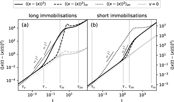
Figure 6. Mean squared displacements of initially mobile tracers. In (a) and (b) we choose  and
and  , respectively. The solid lines denote the MSD of the total density, while the dashed and dotted lines denote the MSDs of the mobile and immobile density, respectively. For comparison, the same is shown in grey for the case without advection. We use the exact expressions of the moments given in appendix
  and
and  as grey lines. In panel (a) we use the same parameters as in figure 4. In panel (b) we use v = 200,
  ,
,  and
and  .
.
Download figure:
Standard image High-resolution imageNow we choose long immobilisations,  , and consider the intermediate immobilisation dominated regime
  . In the absence of advection we found a plateau of the total MSD shown as the grey solid line in figure 6(a). Compared to [54] we here choose a high Péclet number,
  , and keep the time scale separation
  here. The plateau still exists at
  , although at a higher value as shown by the black solid line in figure 6(a). The existence of the plateau comes as no surprise, because the physical mechanism of the plateau remains unchanged. All tracers are initially mobile and have immobilised for
  , as shown in figure 4 for t = 10. When all tracers are immobile the density does not change and hence the MSD remains constant. Analytically, this can be seen most easily from the expressions of the moments in Laplace space


that we obtain from expression (A.5). For  , we have
  , which is a constant. Since the Laplace inverse
 ![$\mathscr{L}^{-1}[1/s] = 1$](https://content.cld.iop.org/journals/1367-2630/25/6/063009/revision2/njpacd950ieqn250.gif) we obtain a constant MSD in this time-domain
we obtain a constant MSD in this time-domain  , where we observe the asymmetric Laplace distribution (23). We emphasise that the plateau exists regardless of the values of v and D. At long times
  the MSD grows linearly with the effective diffusion coefficient
  , as described in section 2.5.
4. Initially immobile tracers
In this section we consider initially immobile tracers. Experimentally, this may correspond to the situation when tracers are released into a microfluidic setup and (part of them) allowed to bind to the sensor receptors. Subsequently, the mobile tracers are flushed out, and then the recording is started. In section 4.1 we report the density for long immobilisations,  , and high Péclet numbers. In section 4.2 we repeat the same steps for short immobilisations,
  . Section 4.3 is concerned with the MSD, and in the fourth subsection appendix J.1 we analyse for which parameters a cubic scaling of the MSD emerges at intermediate time scales.
4.1. Density for long immobilisations
We assume long immobilisations,  , corresponding to the case studied in [54]. We choose a high Péclet number to emphasise the effect of advection, in contrast to the v = 0 case in [54]. At short times
  the propagator for mobile tracers is the same Gaussian as for the case v = 0. Therefore, we obtain the same short-time densities as in the v = 0 case, i.e. a δ-peak at the origin and an additional non-Gaussian distribution.
At short to intermediate times,  , at which t can be shorter or longer than τv
, most initially immobile tracers are concentrated at the origin and only gradually mobilise. This gives rise to the immobile density
, at which t can be shorter or longer than τv
, most initially immobile tracers are concentrated at the origin and only gradually mobilise. This gives rise to the immobile density  . As described in detail in [54], immobile tracers that were initially mobile follow the same density as mobile tracers that were initially immobile, equation (19), up to a factor
  . Therefore, we arrive at the total density for short to intermediate times
for  . The asymptote of the second summand corresponding to the mobile density in expression (31) is shown in figure 7 as the blue dashed line, which nicely matches the simulations and the Laplace inversions for
  and
and  . We note that
  is always normalised,
  , by construction. The same arguments as presented for initially mobile tracers explain the uniform density that appears at intermediate time scales for
  , corresponding to the second panel in figure 7. In the immobilisation dominated intermediate time domain
  the Laplace distribution with additional δ-peak

emerges with the same scale parameter as for initially mobile tracers (23). The prefactor of the asymmetric Laplace distribution is now  , and this asymmetric Laplace distribution is shown in figure 7 as the grey dashed line. The long-time limit does not depend on the initial conditions and follows the same density as the initially mobile tracers, equation (17), as shown by the red dashed line in figure 7 at
  .
.
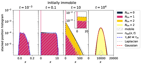
Figure 7. Same as figure 4 for initially immobile tracers. The blue dashed line shows the short-time asymptote (31) and the red dashed line the Gaussian (17) with effective diffusivity  . Parameters:

 v = 100.
Download figure:
Standard image High-resolution image4.2. Density for short immobilisations
We now consider short immobilisations,  . At short to intermediate time scales
  , at which t can be shorter or longer than τv
, the same expression (31) holds as for long immobilisations. This can be seen in figure 8, where the asymptote (31) is shown as the blue dashed line. We find excellent agreement between the histogram based on the simulations and the density (31) for
, at which t can be shorter or longer than τv
, the same expression (31) holds as for long immobilisations. This can be seen in figure 8, where the asymptote (31) is shown as the blue dashed line. We find excellent agreement between the histogram based on the simulations and the density (31) for  , see the first and second panels in figure 8 for
  and
and  , respectively. In contrast to the case v = 0 in [54], a new regime
  emerges, that we call advection induced subdiffusion. The total density follows an exponential distribution, as can be seen from the linear shape of the density in the semi-log plot for
  . To explain this shape we solve the model equations (3) for the advection induced subdiffusion regime times
  , where t can be longer or shorter than τv
. This produces the total density
, where t can be longer or shorter than τv
. This produces the total density

where the integral is identical to expression (25) for immobile tracers that were initially mobile. We obtain the expression

for  and
and  . This comes as no surprise, as in both cases we have the same Gaussian propagator, in which the tracers have varying immobile durations. In the case of initially mobile tracers the immobile duration stems from an immobilisation at t > 0. In the present case of initially immobile tracers the immobile duration arises from the slow release at the origin at t = 0. In both cases the immobile duration is drawn from an exponential distribution with mean
  . The first term in (34) corresponds to initially immobile tracers that have not mobilised up to time t. The second term accounts for the slow release with rate
  and motion in the mobile zone with advection only. The exponential distribution (34) is shown in figure 8 at
  as the grey dashed line, and we find good agreement with the Laplace inversion of
  and simulations.
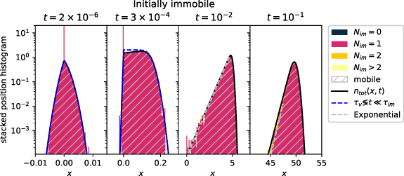
Figure 8. Same as figure 4 for initially immobile tracers and  , i.e.
  ,
,  , v = 500 and D = 1. The exponential asymptote (34) for
  is shown as the grey dashed line for
  .
.
Download figure:
Standard image High-resolution image4.3. Mean squared displacement
We now analyse the MSD of the total density. In appendices E.2.1 and E.2.2 we analyse the MSD of the immobile and mobile density, respectively. We show the MSDs for long and short immobilisations in panels (a) and (b) of figure 9, respectively. From a series expansion of the MSD at t = 0 we obtain the asymptotic MSD at short to intermediate times,

in which t can be smaller or larger than τv
. We compare the asymptote (35) to the full expression of the MSD in figure E2(b) and find very nice agreement. At short times  , the quadratic term dominates and we observe the same MSD as in the case without advection. This can be seen in figures 9(a) and (b). At intermediate times
  the cubic term in the asymptotic MSD (35) dominates. As shown in figure 9 the cubic scaling emerges for short and long immobilisations.

Figure 9. MSDs of initially immobile tracers. In (a) and (b) we choose  and
and  , respectively. The solid lines denote the MSD of the total density, while the dashed and dotted lines denote the MSDs of the mobile and immobile density, respectively. For comparison, the same is shown in grey for the case without advection. As a guide to the eye we show the power-laws
  and
and  as grey lines. The blue dots display the asymptote (36) for the total MSD. In panel (a) we use the same parameters as in figure 4. In panel (b) we use v = 200,
  ,
,  and
and  .
.
Download figure:
Standard image High-resolution imageNow we go to the case of short immobilisation,  , for which advection induced subdiffusion emerges for
  . As described in section 4.2, the total density follows an exponential distribution (34) and a δ-peak at the origin for
  . The MSD of that distribution is given by

for  and
and  , which is shown in figure 9(b) as the blue line. From expression (36) we recover the intermediate time asymptote

implying the same cubic scaling for  as we found from the series expansion of the full MSD (35) for the advection dominated regime. This can be seen in the MSD in figure 9(b). The cubic scaling of the MSD emerges in the domain
  , which limits the parameters to
  . In terms of the Péclet number this implies
  for long immobilisations
  and
and  for short immobilisations
  . A detailed discussion of the parameter regimes and the coexistence of the plateau regime is presented in appendix
In the advection induced subdiffusion domain the MSD (36) reaches the plateau value

These two anomalous scaling regimes shown in figure 9(b), namely, the cubic scaling and the plateau behaviour can be explained as follows. For  the MSD grows due to the slow release and fast advection, where the spread due to diffusion is negligible. When all tracers mobilised at
  , this spread due to advection vanishes, and the distribution moves along the direction of advection without changing the shape significantly. This explains the plateau in the MSD for
  . We highlight that this advection induced subdiffusion is a new behaviour compared to the case without advection. For comparison, we show the MSD for v = 0 in figure 9(b) as the grey solid line. It crosses over from the short-time scaling
  to the long-time asymptote
  without any intermediate regime.
5. Conclusion
We analysed the densities along with the first and second moments of the MIM with exponential Poissonian switching between the mobile and immobile states in the presence of a drift velocity v. The whole dynamic is characterised by the mean mobile duration  , the mean immobile duration
  and the time scale
  , which is related to the Péclet number
  . For
. For  advection plays a negligible role and the process is diffusion dominated, yielding the same results as in [54], where the diffusion regimes were analysed for the advection-free case. In order to highlight the role of advection we choose
  , for which an advection dominated regime emerges for
  . Relatively high Péclet numbers can be achieved in microfluidic setups and in certain geophysical systems. The first moment is proportional to the second moment of the advection-free model, as shown by the second Einstein relation. The second moment of the advection-free model has been discussed in detail in [54]. Therefore, we here concentrated on the discussion of the MSD. In general, for any fraction of initially mobile tracers and an arbitrary fraction
  , we found the same long-time behaviour for
  . The total density follows a Gaussian with an effective advection speed
  and an effective diffusivity
  . Compared to the advection v in the free phase,
  is always smaller. The effective diffusivity
  is always larger than the effective diffusivity in the advection-free case due to the velocity-dependent term. Specifically, for sufficiently high Péclet numbers the effective diffusivity can significantly exceed the diffusivity D in the mobile domain. While
  was reported before [7, 13], we here provided a physical explanation for the additional dispersion due to the variance of durations the tracers spent in the mobile state.
We analysed two specific initial conditions with fully mobile and fully immobile tracers in detail. For initially mobile tracers the advection dominated regime contains two parts. In the first part,  , the MSD grows linearly in time. In the second part of the advection-dominated regime,
  , the MSD grows cubically. This regime is valid for any ratio
  . This can be seen in table 1, where we summarise the main results of the anomalous scaling of the MSD.
Table 1. Main results of anomalous scaling of the MSD. In the second column the short-time asymptotes of the total density's MSD is shown for initially mobile and initially immobile tracers. The cubic term dominates for the time regime given in the third column, with  and
and  . In the fourth column the time regimes of the plateaus are given. For initially immobile tracers this advection induced subdiffusion occurs for large Péclet numbers only.
| tracers initially |

| cubic regime | plateau regime |
|---|---|---|---|
| mobile |

|
|

|
| immobile |

|
|
 for for 
|
For long immobilisations  for initially mobile tracers, and in the advection dominated regime, the density consists of a Gaussian shape of mobile tracers plus a spatially uniform distribution of immobilised tracers. At longer times,
  , we recovered a plateau in the MSD of initially mobile tracers reported in [54], regardless of the presence of advection. In this immobilisation dominated regime the distribution follows an asymmetric Laplace distribution, which decays rapidly in the direction opposite of the advection velocity and falls of slowly in the direction of the advection velocity. In the opposite case of short immobilisations,
  , the total density follows a decreasing Gaussian shape with an increasing exponential tail in the direction opposite of the advection velocity in the whole advection dominated regime
  . This exponential tail is similar to what was found for CTRWs with advection [46].
For initially immobile tracers the advection-dominated regime emerges, as well. This can be seen in table 1, where the series expansion of the MSD is shown. Here, the cubic scaling of the MSD appears in the whole regime  for any ratio of
  and a sufficiently high Péclet number. This is in contrast to the advection-free case reported in [54], where the MSD is close to the Brownian case for short immobilisations,
  . For such short immobilisations the density follows a growing and drifting exponential distribution with an additional peak of immobile tracers at the origin. For later times, we found an advection induced subdiffusion regime
  for high Péclet numbers and short immobilisations. This regime has not been reported previously. Here, the density consists of an exponential distribution with fixed scale parameters, where the mean is moving at a constant speed. For long immobilisations
  , the density follows a spatially uniform distribution for
  . For completeness, we consider an equilibrium fraction of initially mobile tracers in, which naturally occur in experiments, in appendix
Now we put our work into some context. A CTRW with an exponential sojourn time distribution with mean τ and a Gaussian displacement density with non-zero mean µ and variance σ2 was considered in [46]. This model may appear similar to our model with exponentially distributed residence times in the immobile state and advection–diffusion in the mobile state. However, the MSD ![$\langle [x(t)-\langle x(t)\rangle]^2\rangle = \sigma^2t/\tau+\mu^2t/\tau$](https://content.cld.iop.org/journals/1367-2630/25/6/063009/revision2/njpacd950ieqn356.gif) is linear at all times for the CTRW, as shown in appendix L.1. This contrasts the anomalous scaling at intermediate times of the MSD found here. Another formulation of CTRW is the two-state CTRW, in which two transition densities are considered from which steps are drawn in an alternating way [51]. In [51] the long-time asymptotic diffusion coefficient is obtained, which matches our result for a specific choice of parameters. We also mention the case in [52] in which a CTRW is analysed, whose waiting time distribution function is the weighted sum of two exponentials. If one of the exponential distributions has a weight close to unity and a mean that is significantly shorter than
is linear at all times for the CTRW, as shown in appendix L.1. This contrasts the anomalous scaling at intermediate times of the MSD found here. Another formulation of CTRW is the two-state CTRW, in which two transition densities are considered from which steps are drawn in an alternating way [51]. In [51] the long-time asymptotic diffusion coefficient is obtained, which matches our result for a specific choice of parameters. We also mention the case in [52] in which a CTRW is analysed, whose waiting time distribution function is the weighted sum of two exponentials. If one of the exponential distributions has a weight close to unity and a mean that is significantly shorter than  , this model generates the same MSD as the MSD of the total density from the MIM. We stress that the MIM provides additional information in the form of separate mobile and immobile densities. Thus the MIM is not simply the long-space-time limit of the model in [52]. A detailed analysis of the similarities and differences between the MIM and the processes in [51, 52] deserves a separate study.
In contrast to the advection-free case of MIM, where intermittent anomalous diffusion solely arises for mobile tracers for long immobilisations, the anomalous transport behaviours reported here occur for both long and short immobilisations. A condition for this anomalous behaviour is a high Péclet number, which occurs for example in experiments with biomolecules in biosensors [38]. Short immobilisations may occur unintentionally due to unwanted binding to the surface of a flow cell or other experimental boundaries. The resulting transport will be anomalous at intermediate time scales, even if the tracers are only subject to Brownian motion with drift in the mobile state. While the anomalous diffusion and non-Gaussian densities occur at intermediate time scales only, the measurement time is finite in experiments, and the effects may therefore erroneously appear to be an asymptotic phenomenon. In conclusion, we found a variety of anomalous diffusion regimes and non-Gaussian displacement distributions at relevant intermediate time scales in a simple MIM. We emphasise that the model's simplicity is attributed to its dependency on merely two parameters in its dimensionless representation. We finally note that persistent-intermittent anomalous scaling behaviours of the MSD as reported here for seemingly simple Poissonian mobile–immobile dynamics may be relevant for numerous experimental settings. Such scenarios should therefore be included in contemporary data analysis methods by classical observables and machine learning approaches [67–69].
Acknowledgments
We acknowledge funding from the German Science Foundation (DFG, Grant No. ME 1535/12-1). AVC acknowledges the support of the Polish National Agency for Academic Exchange (NAWA).
Data availability statement
No new data were created or analysed in this study.
Appendix A: Solving the MIM model in Fourier-Laplace space
We apply the Fourier–Laplace transform

to equations (3) and obtain the expressions


as well as
with ![$\phi(s) = s[1+\tau_\mathrm{im}\tau_\mathrm{m}^{-1}/(1+s\tau_\mathrm{im})]$](https://content.cld.iop.org/journals/1367-2630/25/6/063009/revision2/njpacd950ieqn358.gif) . Fourier inversion directly produces expressions (4) to (6).
. Fourier inversion directly produces expressions (4) to (6).
From the densities (A.2) to (A.4) we obtain the pth moment ( )
)

in Laplace space. In order to obtain the mobile and immobile moments, we first calculate the non-normalised moments

with  . We then normalise the moment (A.6) in the time-domain with the fractions of mobile and immobile densities,


which we obtain by setting k = 0 in the densities (A.2)–(A.3) in Fourier–Laplace space and calculating the Laplace inversion.
Appendix B: Expressions of the moments
In this section we present the exact expressions of the first and second moments, which are obtained from expression (A.6).
B.1. First moments
For mobile initial conditions we find

and
For initially immobile tracers we find

and

B.2. Second moments
Consider initially mobile tracers ( and
and  ). Then we obtain
and
along with
For initially immobile tracers the moments read
and
Appendix C: Series expansion of moments
The series expansion of the MSDs is shown in table C1.
Table C1. Short to intermediate time expansions for  of the MSD for different fractions of initially mobile tracers
  .
.
| j | series of ![$\langle [x(t)-\langle x(t)\rangle]^2\rangle_j$](https://content.cld.iop.org/journals/1367-2630/25/6/063009/revision2/njpacd950ieqn367.gif) for for 
|
|---|---|

| |
| tot |
![$2Dt-\frac{Dt^2}{\tau_\mathrm{m}}+\left[v^2+D\left(\frac{1}{\tau_\mathrm{m}}+\frac{1}{\tau_\mathrm{im}}\right)\right]\frac{t^3}{3\tau_\mathrm{m}}- \left[2v^2\left(\frac{2}{\tau_\mathrm{m}}+\frac{1}{\tau_\mathrm{im}}\right)+ D\left(\frac{1}{\tau_\mathrm{m}}+\frac{1}{\tau_\mathrm{im}}\right)^2\right] \frac{t^4}{12\tau_\mathrm{m}}$](https://content.cld.iop.org/journals/1367-2630/25/6/063009/revision2/njpacd950ieqn370.gif)
|
| m |
![$2Dt-\frac{Dt^3}{3\tau_\mathrm{m}\tau_\mathrm{im}}+\left[\frac{v^2}{12}+ D\left(\frac{1}{6\tau_\mathrm{im}}-\frac{1}{6\tau_\mathrm{m}}\right)\right] \frac{t^4}{\tau_\mathrm{m}\tau_\mathrm{im}}+\left[3v^2(\tau_\mathrm{im}- \tau_\mathrm{m})+D\left(14-\frac{3\tau_\mathrm{im}}{\tau_\mathrm{m}}-\frac{3\tau_ \mathrm{m}}{\tau_\mathrm{im}}\right)\right]\frac{t^5}{60\tau_\mathrm{m}^2\tau_ \mathrm{im}^2}$](https://content.cld.iop.org/journals/1367-2630/25/6/063009/revision2/njpacd950ieqn371.gif)
|
| im |
![$Dt+\left[\frac{v^2}{12}+D\left(\frac{1}{6\tau_\mathrm{im}}-\frac{1}{6\tau_ \mathrm{m}}\right)\right]t^2+\left[v^2\left(2-\frac{3\tau_\mathrm{m}}{ \tau_\mathrm{im}}-\frac{3\tau_\mathrm{im}}{\tau_\mathrm{m}}\right)+2D(\tau_ \mathrm{im}-\tau_\mathrm{m})\left(\frac{1}{\tau_\mathrm{im}}+\frac{1}{\tau_ \mathrm{m}}\right)^2\right]\frac{t^4}{720 \tau_\mathrm{im} \tau_\mathrm{ m}}$](https://content.cld.iop.org/journals/1367-2630/25/6/063009/revision2/njpacd950ieqn372.gif)
|

| |
| tot |
|
| m |
![$Dt+\left[\frac{v^2}{12}+D\left(\frac{1}{6\tau_\mathrm{im}}-\frac{1}{ 6\tau_\mathrm{m}}\right)\right]t^2$](https://content.cld.iop.org/journals/1367-2630/25/6/063009/revision2/njpacd950ieqn375.gif)
|
| im |
![$\frac{Dt^3}{3\tau_\mathrm{m}\tau_\mathrm{im}}+\left[\frac{v^2}{12}+ D\left(\frac{1}{6\tau_\mathrm{im}}-\frac{1}{6\tau_\mathrm{m}}\right)\right] \frac{t^4}{\tau_\mathrm{m}\tau_\mathrm{im}}$](https://content.cld.iop.org/journals/1367-2630/25/6/063009/revision2/njpacd950ieqn376.gif)
|
Appendix D: Details on subordination
The probability density function  of
of  is calculated in [23] and reads

Here,  and
and  denote the probability of initially mobile and immobile tracers, respectively, to spend in total the duration τ mobile in q mobile periods. The tracer remains immobile for the total duration
  in r immobile periods. The expressions for
  and
and  are given by


and
In geological experiments, typically the mobile density is measured [18]. Similarly to expression (11), we obtain the mobile density
with the probability  to be mobile for a total duration tʹ at time t conditioned to be in the mobile phase at time t. From expression (D.1) we simply need to remove the terms with an additional immobilisation to obtain

The immobile density  and
and  can be defined analogously to expressions (D.6) and (D.7) with

The subordinator  can also be obtained in another way, as we show now. Since i(t) follows a telegraph process, it is easy to see that the probability density functions
  and
and  for the operational time obey the following set of equations
where  and
and  denote the subordinator
  conditioned on the tracer being mobile or immobile at time t, respectively, with
  . Double Laplace transform
  of
of  yields

with ![$\phi(s) = s[1+\tau_\mathrm{im}\tau_\mathrm{m}^{-1}/(1+s\tau_\mathrm{im})]$](https://content.cld.iop.org/journals/1367-2630/25/6/063009/revision2/njpacd950ieqn394.gif) . From
. From  (D.10) we obtain the first and second moments in Laplace space

for p = 1 and p = 2, respectively. We do not provide the lengthy expressions in time domain here. In the long-time  the first moment is given by
  and the second central moment is given by
 ![$\langle [\tau(t)-\langle \tau(t)\rangle]^2\rangle\sim 2\tau_\mathrm{m}^2\tau_\mathrm{im}^2 /(\tau_\mathrm{m}+\tau_\mathrm{im})^3t$](https://content.cld.iop.org/journals/1367-2630/25/6/063009/revision2/njpacd950ieqn398.gif) . Laplace-inversion of
. Laplace-inversion of  (D.10) gives the expression

with the Heaviside step function  .
.
Appendix E: Additional figures and asymptotes of the MSD
In this section we show additional figures of the MSD and develop asymptotic expressions of the mobile and immobile densities. In figure E1 the MSD is shown in addition to the instantaneous diffusion exponent  for initially mobile tracers. For instance the cubic scaling can be seen in panels (c) and (d), where
  takes on values close to three for extended periods. In figure E2 we compare the expressions obtained for intermediate time scales to the exact expressions of the MSD.

Figure E1. MSDs of initially mobile tracers. In (a) and (b) we choose  and
and  , respectively. The parameters are chosen specifically to emphasise the intermediate scaling. The solid lines denote the MSD of the total density, while the dashed and dotted lines denote the MSDs of the mobile and immobile density, respectively. For comparison, the same is shown in grey for the case without advection. Panels (c) and (d) depict the slope α in the double-logarithmic plots from (a) and (b), respectively. In panel (a) and (c) we use the parameters
  ,
,  ,
,  and
and  . In panel (b) and (d) we use
  ,
,  ,
,  and
and  .
.
Download figure:
Standard image High-resolution imageE.1. Mobile initial conditions
We assume initially mobile tracers and obtain asymptotic expressions in sections appendices E.1.1 and E.1.2.
E.1.1. MSD of the immobile density
Now we turn to the MSD of the immobile density. A series expansion of the exact MSD produces

Expression (E.1) implies a ballistic scaling of the immobile MSD for  . This matches the MSD of the uniform distribution (20) of
  shown in figure 4 where the right border moves at a constant speed. The immobile MSD with the ballistic scaling is shown in figure 6(a) as the dotted line. Panel (c) depicts the anomalous diffusion exponent α, which is close to two for
  . Figure 6(a) shows the MSD of the mobile density as a dashed black line. For almost all times
  it coincides with 2 Dt corresponding to the case without advection and Brownian diffusion. The reason for this is that at
  almost all mobile tracers have never immobilised, as shown in figure 4.
E.1.2. MSD of the mobile density
The MSD of the mobile density has the series expansion

The short-time behaviour 2 Dt dominates up to  , as shown in figures 6(a) and (b). The time scale
  is very close to
  in panel (a) and close to
  in panel (b), therefore the t4 scaling is not observed in figure 6. In the appendix in figure E1(a), we choose a higher Péclet number, for which the t4 scaling is distinct. After
  the MSD has a peak and decreases afterwards for some time. This can be explained similarly to the advection free case in [54]. Up to
  , most of the mobile density consists of mobile tracers that have never immobilised. This can be seen in the histogram for t = 0.1 in figure 4, where most of the mobile density follows a Gaussian which is coloured black corresponding to zero immobilisation events
  . When the mobile density mostly consists of tracers that were immobile once the MSD decreases because the leading Gaussian peak is missing.
E.2. Immobile initial conditions
We assume initially immobile tracers and obtain asymptotic expressions in sections appendices E.2.1 and E.2.2.
E.2.1. MSD of the immobile density
From a series expansion of the immobile MSD we obtain the short to intermediate time asymptote of the immobile population,

where t can be shorter or longer than τv
. In figure E2(b) we verify this asymptote and it shows good agreement with the full analytical solution. For a high Péclet number  the quartic term in the asymptotic MSD (E.3) dominates for
  , as shown in figures 9(a) and (b).

Figure E2. Verification of the asymptotes for  in panels (a) and (b) and for
  in panels (c) and (d). The black lines are the exact expressions, while the coloured dotted lines are the corresponding asymptotes. Parameters for (a) and (b): v = 100,
  ,
,  and
and  . Parameters for (c) and (d): v = 200,
  ,
,  and
and  . The blue dots in (a) and (c) correspond to expression (27). The green dots correspond to expression (E.2). The orange dots correspond to expression (E.1). In panels (b) and (d) the blue dots correspond to expression (35), the green dots correspond to expression (E.2) and the orange dots correspond to (E.3).
Download figure:
Standard image High-resolution imageE.2.2. MSD of the mobile density

Appendix F: Calculations for long immobilisations
We consider  in
in  (5), and find the expression

which corresponds in time-domain to the integral

The integral (F.2) has the physical interpretation of mobile tracers following a Gaussian and immobilising with the constant rate  .
.
Appendix G: Density with short immobilisations
For  , the fraction
  of mobile tracers is trapped for a short period τ drawn from
  . This is shown as the red area in figure 5 denoting one immobilisation. Hence, these tracers were mobile for a total period of
  . We convolute this with the propagator for advection diffusion and obtain the expression
with the complimentary error function  . Note that (G.1) is also valid for
  , i.e. also for the case without advection. The seemingly imaginary parts cancel out. Expression (G.1) can be rewritten as
  , which is strictly positive with
  , and it does not oscillate. The
  rather removes the oscillatory part of the
  and the error function approaches unity for large x.
Appendix H: Dependence of  on the model parameters

We now analyse the dependence of the effective diffusion coefficient on the model parameters. In section 2.3 we show that only two dimensionless parameters characterise the model, namely the Péclet number and  . We use the decadic logarithms of these parameters as the abscissa and ordinate in figure H1. The logarithmic colour map encodes the ratio
  for
for  . Outside that region
  is smaller than D, as in the case without advection in [54]. For high Péclet numbers
  takes on high values depending on
  . Now we analyse this dependence in more detail. For D > 0 we now analyse the ratio
  , that depends on
  and
and  . For
. For  we find the expression

Figure H1. Contour plot of  with the logarithm of the Péclet number
  as abscissa and the logarithm of
  as ordinate. The colour map encodes the increase of the effective diffusion coefficient
  (equation (15)) as compared to the bare value D. In the white area
  . The solid grey lines (corresponding to values
  ) are obtained from expression (H.1). The asymptotes (H.2) and (H.3) for
  for long and short immobilisations are shown as blue and white lines, respectively. In the domain enclosed by the dashed line the time scale
  is not smaller than
  or
or  , respectively. It can be seen that
  only occurs outside this domain, i.e. when
  is smaller than
  and
and  .
.
Download figure:
Standard image High-resolution image

which is the Péclet number as a function of  . It is shown for a range of c values in figure H1 as solid grey lines and matches the colour plot. We obtain the asymptotes

and

from expression (H.1). The asymptote (H.2) is shown as the blue line at the top of the map in figure H1. For the lower bound in the map we choose c = 2 and depict the asymptote  as a white line in figure H1. Both asymptotes are parallel to the exact expressions shown as grey lines.
Appendix I: Parameter regimes for anomalous diffusion for initially mobile tracers
I.1. Parameter regimes for superdiffusion
Here we analyse for which parameter regimes the cubic scaling (27) of the total MSD appears for initially mobile tracers. First, long immobilisations are assumed in section appendix I.2
 , followed by short immobilisations in section appendix I.3.
I.2. Long immobilisations
A necessary condition for the cubic regime to emerge is that the lower bound  of the time regime is smaller than the upper bound
  . We define t3 as the duration between the upper and lower bound. This restricts the parameter space in which the cubic regime appears to positive values of the time difference t3. As shown in section 2.3, the whole parameter space can be spanned by the Péclet number
  and the ratio
  . We use the decadic logarithm of these quantities as axis for a map in figure I1, similar to figure H1. The border of the region with
  in the top right of figure H1 is shown as a black dotted line. We notice that
  is a necessary condition for
  . We analyse the parameter space for
  first and for
  afterwards. Rearranging the condition
  for the Péclet number reveals the lower bound
  independent of
  . Indeed, the black dotted line for
  is vertical in the map (I1) for
  , indicating no dependence on
  in that regime.
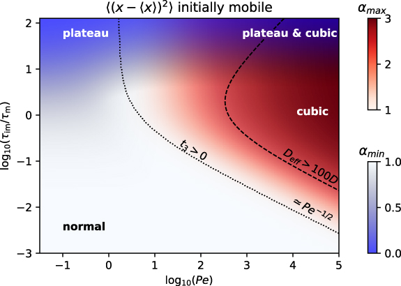
Figure I1. Map with sub- and superdiffusive regimes. The y-axis is chosen as  and is an indicator for the strength of the effect of the immobilisations on the MSD. The x-axis is the logarithm of the Péclet number
  . Both parameters span the full phase space, as described in section 2.3. Depending on the parameters, the MSD of the total density with initially mobile tracers has a cubic scaling for
  and a plateau for
  . We quantify the existence of the cubic scaling with the maximum value of the anomalous diffusion exponent α for each point in the map. We show this
  with a red colour coding. The black dotted line shows the border of the domain where the duration of the cubic scaling is larger than zero, i.e.
  . It has the asymptote
  for large Péclet numbers. The black dashed line shows the contour line, at which
  . It has the same asymptotic scaling
  for large Péclet numbers and short immobilisations. For short immobilisations, i.e. negative ordinates, the shape of the read area follows the same asymptote. We quantify the existence of the plateau with the minimum value of the anomalous diffusion exponent for each point in the map. We show this
  with the blue colour coding. The top left corner corresponds to the parameters discussed in [54]. In the top right corner we have a coexistence of the cubic scaling and the plateau in the MSD. In the white area both
  and
and  are close to unity, i.e. the MSD is close to linear at all times.
Download figure:
Standard image High-resolution imageSo far, we looked at the necessary condition that the lower bound for the interval of the cubic regime is lower than the upper bound. Another approach is to analyse the instantaneous anomalous diffusion exponent  . It can be obtained by calculating the slope in a double-logarithmic plot. This is shown in figure E1(c), where α remains close to unity for
  and reaches the value three for
  . The alternative criterion for the cubic regime to exist is then simply that the maximum value of
  is close to three. With this definition of
  , superdiffusive parameter regimes are shown with the red colour-coding ranging from one to three in figure I1. This means that the more intense the red in an area is, the closer the parameters are to the asymptotic limits in which the cubic regime emerges. We notice that the red area lies entirely in the region with
  and its border follows the same asymptote
  for
for  . The cubic regime appears both for
  and for
  for long immobilisations
  and for
  , as shown in the top right corner of the map in figure I1. For reference, a contour plot of
  is shown in figure H1. The reason for the appearance of the cubic regime regardless of the ratio
  is the existence of the plateau for
  , which we explain now in detail. We know that regardless of the ratio
  the MSD of initially mobile tracers has the asymptote 2 Dt for short times
  . In the long-time limit it has the asymptote
  . The MSD of the total density is a strictly monotonic function. This means that if
  , any growth faster than linear must be compensated by a regime with a sublinear growth. This slower than linear growth arises for long immobilisations only and constitutes the plateau for a sufficiently large ratio
  .
.
I.3. Short immobilisations
Finally, we analyse the case of short immobilisations,  . The same series expansion of the total MSD holds as in the case with long immobilisations (27). The difference between the upper and lower bound of the cubic scaling is therefore
  . Notably, the duration of the cubic regime is shorter as compared to the case with long immobilisations in figure 6(a), because
  is close to the lower bound
  for
for  . We emphasise that the cubic regime appears for short immobilisations, whereas for the case without advection the MSD is close to normal, as shown by the grey line in figure 6(b). For
  , i.e. for negative ordinates in figure H1, the condition
  simplifies to
  . This means that for each ratio
  there exists a lower bound for the Péclet number for the cubic regime to exist. Indeed, the black dotted line on the map in figure I1 for
  has the asymptotic scaling
  for
for  . The cubic regime appears for
  only, i.e. only in the top right part from the black dashed line in figure I1. In figure I1 the red colour denotes the maximum anomalous diffusion coefficient
  . The condition
  has the same asymptotic regime
  for
for  , as shown by the black dashed line in figure I1. For
  the dark red region with
  close to three is almost entirely contained within this region. This means that for
  the cubic regime always coexists with
  . In contrast, we found that the cubic regime appears regardless of the ratio
  for long immobilisations.
In addition to the maximum value of the instantaneous anomalous diffusion exponent, we consider the minimum value  in figure I1, in which values close to zero correspond to very slow intermediate growth, i.e. a plateau. This allows us to analyse how the plateau at
  is influenced by the presence of advection and the cubic regime. The coexistence of the cubic regime and the plateau can be seen in the MSD in figure 6(a). The top left blue corner in figure I1 corresponds to the case considered in [54] with long immobilisations and (almost) no advection. The blue subdiffusive area does not significantly change for growing Péclet numbers and it overlaps with the red superdiffusive region in the top right corner of the map in figure I1. In the lower left part of figure I1(a) white area dominates, in which diffusion is close to normal, with both
  and
and  close to unity. This can be seen from the solid grey line in figure 6(b).
Appendix J: Parameter regimes for anomalous diffusion with initially immobile tracers
J.1. Parameter regimes for cubic MSD and advection induced subdiffusion
In section 4.3 we found an anomalous scaling of the MSD, and now we analyse for which values of the Péclet number and the characteristic time scales the cubic scaling of the MSD (35) emerges at intermediate times. The cubic term dominates for  . This implies the time scale separation
  . For long immobilisations
  the parameter space for the cubic scaling to occur is therefore restricted to
  . This can be seen in figure J1 in the top right corner, where we show the decadic logarithm of the Péclet number as the abscissa and
  as the ordinate. The red colour coding denotes the maximal anomalous diffusion coefficient, which is close to three in that top right region. For clarity, the contour line for
  is shown. For short immobilisations,
  , the cubic term in the asymptote (35) dominates for
  , which limits the parameter space for the cubic scaling to occur to
  . This can be seen in the map in figure J1, where the relation
  is shown as a dashed black line. Below this line no cubic scaling is possible, meaning that for a given Péclet number the fraction
  needs to be sufficiently small.

Figure J1. Map with sub- and superdiffusive regimes, same as figure I1 for initially immobile tracers. The y-axis is chosen as  and is an indicator for the strength of the effect of the immobilisations on the MSD. The x-axis is the logarithm of the Péclet number
  . Both parameters span the full phase space, as described in section 2.3. Depending on the parameters, the MSD of the total density with initially mobile tracers has a cubic scaling for
  and advection induced subdiffusion for
  . We quantify the existence of the cubic scaling with the maximum value of the anomalous diffusion exponent α for each point in the map. We show this
  with a red colour coding. The black dashed line shows the scaling
  for large Péclet numbers. We quantify the existence of the advection induced subdiffusion by the minimum value of the anomalous diffusion exponent for each point in the map. We show this
  with the blue colour coding. The top left corner corresponds to the parameters discussed in [54]. In the bottom right corner we have a coexistence of the cubic scaling and the plateau in the MSD. In the white area
  is close to two and
  is close to unity. The white contour lines for
  and
and  serve as a guide to the eye.
Download figure:
Standard image High-resolution imageAfter the cubic scaling an advection induced subdiffusion regime may emerge. The time-domain of the subdiffusion is given by  . Therefore, the subdiffusive regime appears only for short immobilisations,
  . Furthermore, the condition
  translates to
  , shown as the dotted line in figure J1. This restricts the parameter space for the plateau. It is bound by
  , corresponding to the horizontal boundary in figure J1. In the map in figure J1 we show
  for the total MSD as a blue colour map and observe a region with
  in the bottom right corner for a high Péclet number and short immobilisations. As a guide to the eye we show a contour line for
  . A corresponding MSD is shown in figure 9(b), where a plateau occurs for
  . This is a new behaviour that does not occur in the case without advection, as is shown by the grey line in figure J1 for a small Péclet number.
Appendix K: Equilibrium initial condition
We assume the equilibrium fractions  and
and  and consider the MSD of the total density. It is shown in figures K1(a) and (b) as the solid black line for long and short immobilisations, respectively. The densities are given by adding the densities for mobile and immobile initial conditions with the corresponding equilibrium fractions as factors. The MSD is not a linear function and does not follow a linear combination of the initially mobile and immobile MSDs. In contrast to the case without advection in [54], the MSD is no longer linear at all times, and we observe a quadratic scaling for
  . A series expansion yields the asymptote for intermediate times
  , where t can be shorter or longer than τv
,
, where t can be shorter or longer than τv
,

Figure K1. Same as figure 6 for equilibrium initial conditions  . In contrast to the case with v = 0 in [54], the MSD of the total density (solid lines in (a) and (b)) are no longer linear at all times. A quadratic scaling emerges at
  . The MSD of the mobile density is identical to the MSD of the total density with initially mobile tracers in figure 6.
Download figure:
Standard image High-resolution image

The quadratic term dominates over the linear term for  . This is shown in figures K1(a) and (b). In panels (c) and (d) the instantaneous anomalous diffusion exponent is displayed, which is close to two in this domain. Note that for long immobilisations
  . The quadratic scaling emerges for long immobilisations
  for
for  and for short immobilisations for
  .
.
As described in [54], the MSD of the mobile density with equilibrium initial conditions is identical to the MSD of the total density with mobile initial conditions. We discussed this case in detail in the main text. The same holds for the MSD of the immobile density. For an equilibrium fraction of initially mobile tracers the density is given by the linear combination of the results for mobile and for immobile initial conditions.
Appendix L: Comparison to CTRW
In this section we compare our results to three versions of CTRWs. For didactic purposes, we start in appendix L.1 with the classical CTRW with exponentially distributed waiting times. In appendix L.2 we compare our model to the two state CTRW [51]. Finally, in appendix L.3 we compare our model to a CTRW in which the waiting times are drawn from a waiting time distribution containing two exponential distributions [52].
L.1. Classical CTRW
We here compare the results obtained from the MIM (3) to a CTRW with advection and exponentially distributed sojourn times. The relation between MIM and CTRW has been discussed in detail, for example, in [13, 48, 70]. Let us define the sojourn time density  and the Gaussian displacement density
  with mean µ and variance σ2. This corresponds to the model considered in [46]. In [71] the solution of the density function
  in this CTRW framework is given as
for µ = 0. We incorporate the non-zero mean µ and obtain the solution
Let us turn to the moments of  (L.2). The fist moment is given by
In the same way we obtain the second moment

resulting in the MSD

which is linear at all times, in contrast the results obtained from our model.
L.2. Two-state CTRW
In this section we compare our model to the two-state CTRW introduced in [51] in which two transition densities

are present with average speeds vi
and diffusion constants Di
. In an alternating way jumps are drawn from  and
and  . The long-time diffusion coefficient presented in [51] is given by
with  and
and  ,
,  . The long-time effective diffusion coefficient (L.7) matches our result (15), if we formally choose
  ,
,  ,
,  ,
,  ,
,  and
and  .
.
L.3. Double exponential CTRW
In this section we compare our model to the CTRW analysed in [52], in which the waiting time distribution function is given by the weighted sum

of two exponentials, where  and
and ![$p\in [0,1]$](https://content.cld.iop.org/journals/1367-2630/25/6/063009/revision2/njpacd950ieqn608.gif) . The jump length distribution we consider is given by the Gaussian
. The jump length distribution we consider is given by the Gaussian

with mean µ and variance σ2. Note that in [52]  is restricted to the case µ = 0. Formally, we choose the parameters
  ,
,  , and
, and  . We stress that this means that
  and
and  does not have the meaning of the mean residence time in a mobile state. By choosing
  and
and  close to unity there is a high probability to draw from the exponential distribution with short mean duration. This effectively models the Brownian motion of a tracer in the mobile state. After each step, the tracer immobilises with probability
  . If there was no waiting time drawn from the long exponential, on average, there are
  steps at time t. This gives an effective immobilisation rate of
  , which is the same as in MIM. In figure L1 we compare the MSD of MIM for
  ,
,  , v = 0 or v = 10 and D = 1 with simulations of CTRW with
  ,
,  ,
,  and
and  . We find good agreement at all times for the advection-free case, while the CTRW yields higher values than MIM for
  in the case with advection.

Figure L1. Comparison of the MSD from MIM and CTRW with double exponential waiting time [52]. CTRW data originate from simulations and the full expressions from B are used to evaluate the MSDs of MIM.
Download figure:
Standard image High-resolution imageThe reason why the MSDs are identical in the advection-free case and not in the case with advection can be understood by considering the MSD in terms of step numbers n [66]

where  , as introduced in section 2.5. We emphasise that expression (L.10) is exact. From expression (L.10) we see that in the advection-free case
  only the mean number of steps is relevant for the MSD and not the variance of step numbers. Indeed, in figure L2 we show the mean number of steps
  (calculated by setting D = 0), where the dots for CTRW and the line for MIM overlap at all times. Therefore, the MSDs in the advection-free case of CTRW and MIM in figure L1 are equivalent. In contrast, in the case of advection, the variance of step numbers
  couples to the MSD, as can be seen in expression (L.10). The variance of step numbers differs for
  . We explain this as follows. If a tracer is in the mobile state of MIM, it will have a fixed number of steps
  at time t. The stochasticity of step numbers arises solely from immobilisations. By setting D = 0 we obtain a cubic short-time growth of the variance from the short-time asymptote (27). In contrast, in the CTRW case, the number of steps is random even in the case of a simple CTRW with only one exponential waiting time distribution, as described in appendix L.1. It can be seen in the variance of CTRW (L.5) for σ = 0 and µ = 1, where the variance of step numbers grows linearly. This is due to the fact that after each step a random waiting time is drawn from the exponential distribution. Therefore, the variance of step numbers is higher for small times and hence the MSDs of MIM and CTRW do not overlap for
  , as shown in figure L1. We point out that the disagreement between the MSD of MIM and CTRW with advection lasts until
  , which is notably larger than the chosen
  .
.
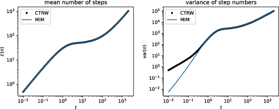
Figure L2. Mean number of steps and variance of step numbers for CTRW with double exponential waiting time [52] and MIM. CTRW data originate from simulations and the full expressions from appendix B are used to evaluate the MSDs of MIM. It is seen that both models shows perfect agreement in the drift-free case, for the specific choice of parameters indicated after equation (L.9), whereas in the presence of a drift, the models converge only in the long time limit.
Download figure:
Standard image High-resolution imageFootnotes
- 5
We use the term 'residence times' in the mobile or immobile state to avoid confusion with the waiting times in a continuous time random walk.
- 6
Later we will demonstrate that the transient anomalous diffusion regime can assume substantial time spans with an approximately constant anomalous diffusion exponent.
- 7
The Gaussian distribution
, that only applies in the long-time limit, in principle allows for negative numbers of steps. However, they asymptotically vanish, because the width of the distribution vanishes compared to the mean. We quantify this using the coefficient of variation of step numbers for . Note that here means equivalence in distribution. - 8


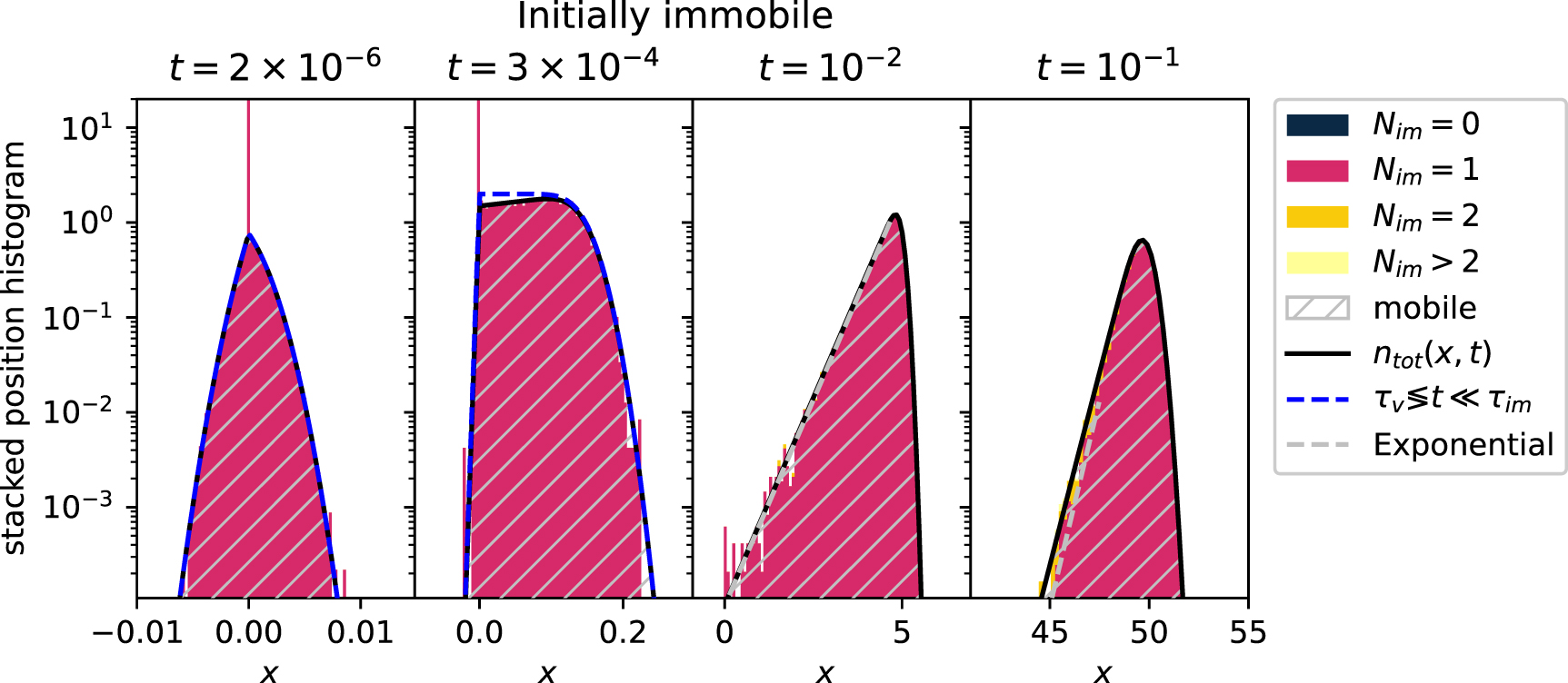