


Abstract
Using molecular dynamics simulations, we study a driven, nonadditive binary mixture of spherical particles confined to move in two dimensions and immersed in an explicit solvent consisting of point particles with purely repulsive interactions. We show that, without a drive, the mixture of spherical particles phase separates and coarsens with kinetics consistent with an Ising-like conserved dynamics. Conversely, when the drive is applied, the coarsening is arrested and the system develops large density fluctuations. We show that the drive creates domains of a characteristic size which decreases with an increasing force. Furthermore, we find that these domains are anisotropic and can be oriented either parallel or perpendicular to the drive direction. Finally, we connect our findings to existing theories of strongly-driven systems, pointing out the importance of introducing the explicit solvent particles to break the Galilean invariance of the system.
Export citation and abstract BibTeX RIS
1. Introduction and background
In both simple fluids and in more complex, colloidal and polymer systems, excluded volume effects play an important role. A general model describing such systems is the nonadditive binary hard sphere mixture, in which spheres A and B with radii aA
and aB
, respectively, have a mutual collision diameter  , where
  characterizes the nonadditivity of the mixture. This model describes, among many other examples, polymer-colloid interactions (the Asakura–Oosawa mixture [1–3]), phase separation in fluid mixtures at high pressures [4], and liquid–vapor transitions (the Widom–Rowlinson model [5]). Here, we consider a symmetric mixture of two particle types A and B in which
  , with
  . Such a situation can be realized, for example, in mixtures of nanoparticles decorated by polymer brushes. These particles have applications to self-assembled materials, and generally have repulsive entropic interactions [6]. Various polymers may be grafted onto a nanoparticle surface, including immiscible ones such as polystyrene and poly methyl methacrylate (PMMA) [7]. Mixtures of this type are known to phase separate, with kinetics consistent with the Ising universality class [8]. Additionally, driven binary mixtures have also been shown to exhibit interesting phenomena including giant diffusion enhancement [9], segregation [10], enhanced density fluctuations [11], and lane formation [12], to name a few. Here we aim to establish some general features of the driven, nonadditive mixture immersed in a 'solvent' consisting of repulsive point particles.
Although the equilibrium phases of such mixtures are reasonably well-understood, not as much is known about mixtures when driven out of equilibrium. Even single-component driven systems, despite decades of study, continue to present surprises and challenges for both theory and experiment [13–15]. The Katz–Lebowitz–Spohn (KLS) model [16, 17], a lattice model of a single species gas with attractive interactions (exhibiting a liquid–gas transition), is perhaps the best-studied model with a driven, non-equilibrium steady state. In this case, an applied field orients dense liquid domains at low temperature along the field direction. More recent studies [18, 19] demonstrated that a lattice gas model of a binary mixture of particles with repulsive interactions exhibits striped order perpendicular to the drive direction. These models and associated classes of driven systems largely lack experimental realizations, although it is clear that driven colloidal systems are promising avenues for testing these theories [20].
In this work, we attempt to bridge the gap between the theoretical, lattice-model-based results on the driven, nonadditive binary mixtures and experimental observations by studying more realistic, molecular dynamics (MD) simulations which may, in principle, be practically realized. Specifically, we consider MD simulations of a (nonadditive) mixture of two colloids A and B immersed in a collection of solvent point particles S with repulsive interactions. All particles are confined to move in two dimensions, which could be realized experimentally by depositing the colloids on an aqueous interface. We apply a uniform force to the colloidal particles and achieve a steady velocity, mediated by an opposing friction force provided by the S particles. Such a drive may be created, for example, by an applied flow, an electric field for charged colloidal particles, or a magnetic field [21]. Selective snapshots of particle configurations are shown in figure 1 for low ( ) and high (
 ) colloidal particle densities ρ (given as the area fraction of the simulation box occupied by the colloidal particles). At large particle densities, our mixture phase separates in the absence of a force. Similar phase separation has been observed experimentally for colloids of different sizes [22].

Figure 1. A binary colloidal mixture in two dimensions, simulated for 108 time steps at different particle densities ρ and applied forces F. Each box contains 800 orange A and 800 blue B particles with radius 5σ, where σ = 1 is a length scale described in section 2. The simulation box size L × L is varied to get a low ( in panels (a), (b)) or high (
 in panels (c), (d)) particle density ρ, given as the simulation box area fraction occupied by the colloids. We initialize each system with a square grid of well-separated colloidal particles, with the A and B types assigned randomly (i.e. a mixed initial condition). When F = 0, the mixture coarsens over time, as long as the particle density is sufficiently large (panel (c)). If the particle density is low (panel (a)), the two species A and B do not phase separate. With an applied force F > 0, the system reaches a non-equilibrium steady state characterized by large density fluctuations and arrested coarsening (right panels).
Download figure:
Standard image High-resolution imageAs discussed in more detail below, we find that driving the mixture of particles has two major effects: first, the phase separation between colloidal species is arrested at a characteristic length scale that decreases with an increasing applied field magnitude. Second, the colloidal system develops large density fluctuations in the form of dense 'lanes' or anisotropic clusters separated by lower-density regions. This density distribution is reminiscent of the particle clustering observed in the driven single-component lattice gas (the KLS model). The paper is organized as follows: in the next section, we present the details of MD simulations. In section 3, we explore the structure of the domains of different colloidal species, focusing on what happens to the coarsening behavior in the presence of the applied force. In section 4, we consider the overall particle density distribution changes under an applied field. We discuss these results and conclude in section 5.
2. Model
We consider two colloid particle types A and B. We apply a uniform force F to these particles and introduce a compensating friction force  to each particle (with v the particle velocity, M the particle mass, and γ the friction coefficient). This allows the system to establish a non-equilibrium steady state. A uniform force alone, however, would simply introduce a uniform velocity
  to all the particles. Such a uniform velocity would put the system in a moving reference frame, making it otherwise indistinguishable from the undriven case
  . Thus, to break the Galilean invariance, we introduce a third particle type: a solvent point particle S with mass m which does not experience the applied force F. These solvent particles establish a preferred 'rest frame' and provide additional friction to A and B particles via the repulsive interactions. Therefore, our MD simulations contain three particle types:
  .
.
All three kinds of particles interact via truncated Lennard-Jones potentials, approximating hard-core, repulsive interactions. The colloidal particles A and B are spheres, for which the associated potentials have been analytically determined previously [23, 24]. The solvent S is modeled as a collection of point particles with purely repulsive interactions. All particle interactions between particle types α and β (a center-to-center distance r apart) are captured by potentials  which, in units of
  , read
where  , and aα
is the particle radius, as illustrated in figure 2(a). Here, without loss of generality, the length σ is set to unity and all distances are determined in units of σ. The factors
, and aα
is the particle radius, as illustrated in figure 2(a). Here, without loss of generality, the length σ is set to unity and all distances are determined in units of σ. The factors  are appropriately chosen constants. For self-interactions between colloidal particles (WAA
and WBB
in equation (1)), we set
are appropriately chosen constants. For self-interactions between colloidal particles (WAA
and WBB
in equation (1)), we set  and
and  . The repulsive interaction between colloids, WAB
, is modeled by setting
. The repulsive interaction between colloids, WAB
, is modeled by setting  and
and  , so that the colloids appear as larger spheres to one another, introducing a 'nonadditivity' to the A and B particle mixture. The solvent-colloid interaction,
  , has
, has  and
and  , with
  . Finally, the solvent self-interaction potential WSS
has
. Finally, the solvent self-interaction potential WSS
has  and
and  in equation (1). Each interaction potential
  is truncated (held constant) for all
  , with
  chosen to be the minimum of the interaction potential, so that all potentials
  smoothly approach a constant value at
  . The truncation distances for the various interaction types read:
  ,
,  ,
,  , and
, and  . Note that these truncation distances
  are all slightly larger than
  , meaning that the repulsive interactions act over a narrow range of distances. The interaction potentials
  for the different choices of α and β are shown in figures 2(b) and (c). Note the sharp increase in the potentials
  at values of r near
  . This divergence scales as
  (as in the repulsive portion of the Lennard-Jones potential), with
  as shown in figure 2(c). These purely repulsive potentials, as derived from the Lennard-Jones potential, are also known as Weeks–Chandler–Anderson potentials [25].

Figure 2. (a) Schematic of the particle interactions in our molecular dynamics simulation. The center-to-center particle separation is r and  are the particle radii. Colloids A and B have finite radii
  when interacting with particles of the same type and larger radii
  when interacting with particles of the opposite type. The solvent particles are repulsive point particles with
  (i.e. with a self-interaction potential WSS
that diverges at r = 0). (b) Plot of the interaction potentials
(i.e. with a self-interaction potential WSS
that diverges at r = 0). (b) Plot of the interaction potentials  as given in equation (1) for various interaction types between the A, B colloids and the solvent particles S. Note the sharp increases in the potential energy, modeling a hard-core repulsion. (c) Interaction potentials
  plotted near the strongly repulsive region. Each interaction has a divergence at
  . The potentials diverge approximately as
  , as in the repulsive portion of a Lennard-Jones potential.
Download figure:
Standard image High-resolution imageWe implement the MD in LAMMPS, making use of parallelization on graphics processing units (GPUs) [26, 27]. In addition to the interaction potentials in equation (1), each particle experiences a random force and a friction due to a Langevin thermostat [28]. We also introduce solvent particles S which do not experience the applied force, but allow for the colloidal particles to dissipate the applied force via collisions. All particles move under constant volume and temperature, where the temperature is maintained by coupling the system to the thermostat, such that the motion of each particle  can be described as

where mi
is the particle mass,  is the particle velocity, and
  denotes the net deterministic force acting on the
  particle, as derived from the interaction potential in equation (1). The thermal fluctuations are implemented via a stochastic force
  with Gaussian, white noise components, zero average value
  , and correlations
  . The friction coefficient γ is set to γ = 1 τ−1 where τ is the reduced time unit
  . The mass of A and B particles is
  , where
  is the solvent particle mass. An external force with a magnitude F ranging from 0 to 2.0
  is applied to A and B particles in the
  direction. Note that the thermostat is applied in both x and y directions for the solvent particles S but only in the
  direction for colloidal particles A and B, with the x component of the associated random force set to zero. A similar technique was implemented when performing MD under shear conditions [29, 30]. Removing the thermostat (both the friction and the random force) along the drive direction ensures that the applied force is uniform for all colloidal particles. Periodic boundary conditions in both directions are implemented.
The systems were initialized with a random distribution of A and B particles with locations initially on a square grid. The small solvent particles were then added in as a dilute suspension which was rapidly compressed to a fixed solvent number density. We used a total of 1600 colloidal particles (800 per species) and a variable number of solvents, depending on the overall simulation box size which was used to vary the colloidal density. For the low density systems in figures 1(a) and (b), we have 274 888 solvent particles and a box size L × L with L = 780, while the higher density systems in figures 1(c) and (d) have 82 418 solvent particles and L = 520. The velocity-Verlet algorithm with a time step of  was used for integrating the equations of motion in equation (2) for these initial conditions. The simulations proceeded up to times of at least
  (108 total time steps). We will now set
  for convenience and report times in units of τ and energies (forces) in units of
  (
( ).
).
We verified that the explicit solvent provides a friction force along the drive direction by calculating the colloidal particle velocities as a function of the applied force F. We found that the average velocity and pressure rapidly approach constant values, on a time scale shorter than 104 (early in the simulation runs). We find a linear increase of the colloidal particle velocity with F, as shown in the inset of figure 3(a), so that  , with
  an effective friction coefficient supplied by the small solvent particles S along the drive direction. We find that the friction generally increases with decreasing colloidal particle density. The relationship is shown in figure 3(a). This makes sense as, at lower densities, there are more solvent particles available to provide friction for each colloidal particle. At higher densities, the colloids crowd out the solvents. This is also evident in the velocity snapshots in figure 3(b), where we observe that large, dense clusters of colloidal particles move faster than the more dilute regions for both high and low density systems. We will explore these density variations in more detail section 4. For the lower density ρ ≈ 0.2065, we find a friction coefficient
  . For the higher density ρ ≈ 0.4647, we find
  . Note that these coefficients are about half of the friction coefficient γ = 1 supplied by the Langevin thermostat in the direction perpendicular to the drive. It would be possible to increase
  by supplying more solvent particles, which would cost significant computational resources.
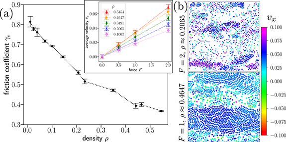
Figure 3. (a) Effective friction coefficient  of the colloidal particles in the applied force direction for various colloidal particle densities ρ. The coefficient is determined by fitting the average colloidal particle velocity
  versus the applied force magnitude F, as shown in the inset:
  . The velocity is calculated over simulations frames in a time interval
  , with error bars indicating the standard deviation in this average from frame to frame. (b) Snapshots of MD simulations at
  with an applied force F = 2 and low particle density (top panel) and at F = 1 with high particle density (bottom panel). The particles are colored according to their velocity vx
in the direction of the force. The colloidal species for the top and bottom panels are shown in figure 1(b), (d), respectively. Note that the repulsive interactions generate faster-moving dense colloidal particle clusters or 'lanes'.
with an applied force F = 2 and low particle density (top panel) and at F = 1 with high particle density (bottom panel). The particles are colored according to their velocity vx
in the direction of the force. The colloidal species for the top and bottom panels are shown in figure 1(b), (d), respectively. Note that the repulsive interactions generate faster-moving dense colloidal particle clusters or 'lanes'.
Download figure:
Standard image High-resolution imageWe have also explored the effects of removing the thermostat entirely from the colloidal particles A and B. We find no qualitative differences and have opted to keep the thermostat in the perpendicular direction throughout the rest of the paper. In addition, we used a momentum-conserving thermostat and found that, in this case, the applied force continuously supplies energy into the system so that both the colloids and solvent particles accelerate, never reaching a stable velocity. It would be interesting to explore the effects of modifying the thermostat in the future.
It is clear that our explicit solvent is compressible and has density variations, leading to the different effective frictions for the colloids as shown in figure 3(a). In an experiment, the colloidal mixture would likely have an incompressible solvent (e.g. water). In this case, hydrodynamic interactions will generate inter-particle interactions between the colloids. For example, moving colloids will generate hydrodynamic flows which can entrain adjacent colloidal particles [31], also effectively decreasing the friction of denser particle clusters. So, although our MD simulations are closer to experimental realizations than previous studies of this system using a lattice [18, 19], there may be important differences. It may be necessary, for example, to add small particles to the colloidal mixture in an experiment to generate the effects provided by our solvent particles S.
3. Coarsening colloids
We begin by looking at colloidal mixtures with no applied force, which we expect to coarsen at sufficiently high density. It is easier to analyze such structures in Fourier space, so we calculate the static structure factors  associated with the 'charge' (−) and density (+) of the colloidal species. Specifically,
where we sum over the N colloidal particles at locations ri
. Here, the weights for the charge structure factor are  if colloidal particle i is of type A or B, respectively. Conversely, for the density structure factor, we have equal weights
  for both types. It is possible to average over many times t to get better statistics for these structure factors, although one must be careful that the static structure factor does not evolve substantially over time. This works best for larger force values for which the coarsening is arrested, as described in the next section. The structure factors are calculated on a square grid in q-space, with spacing
  (in units of
  ).
).
Note that our definitions of  in equation (3) have a constraint at
  :
:  . For equal numbers of A and B particles, this means
  and
and  exactly. This creates an issue as these constraints generate discontinuities in our structure factor measurements. We therefore replace the values of
  at the
  grid site with the value at a neighboring grid site. The structure factors near
  , then, become smoothly-varying. Also, due to the computational difficulty in running these simulations, we were limited to using single simulation runs per condition (colloidal density, force, etc). We used system sizes of at least
  , in units of the Lennard-Jones distance σ. Structure factors calculated from single runs in this way are noisy in the q-space. Therefore, in addition to the time-averaging, we perform a smoothing of the structure factor results by convolving the structure factor with a Gaussian kernel with standard deviation
  . The removal of the
  discontinuities in
  is also helpful in this regard. Finally, we checked that larger system sizes did not significantly modify our results by running some of the systems at twice the (linear) system size L. For example, we checked that the structure factor calculation yields compatible results for box sizes L × L with L = 520 and L = 1040 for the dense colloidal mixtures (ρ ≈ 0.4647).
First, we consider results for the 'charge' structure factor  at large particle densities and F = 0. Here, we would expect domains of
  and
and  particles to coarsen, much like an Ising model with conserved dynamics at low temperature. Without an applied drive to specify a direction, we expect isotropic domains in our simulation and a circularly symmetric average structure factor
  , which is what we find, apart from some fluctuations, in the color maps of figure 4(a). As shown in the bottom panel, the 'ring' of the structure factor at
  gets smaller with increasing time and more difficult to resolve. This is expected for a coarsening system. We can track the position of the peak more systematically by performing a circular average
  , as shown in figure 4(b). We find that the shift in the peak is consistent with the Lifshitz–Slyozov–Wagner coarsening characteristic of conserved dynamics [32, 33], for which
  . We also show in the inset of figure 4(b) the characteristic length scale
  associated with the peak at
  . The red dashed line indicates the
  scaling. Note that at the larger times t, the scale
  approaches values close to the system size, so we expect to see finite size effects at these larger times. At smaller densities, such as those shown in figure 1(a) where the colloidal species remain disordered, we find a similar behavior except that at long times t, the peak stops growing and shifting toward smaller q values. Instead, we approach a steady state with a fixed peak corresponding to the average domain size in the disordered phase. We may thus expect a phase transition in this system (from a phase with mixed A and B particles to a phase where the particles phase separate into distinct A and B domains) somewhere between ρ ≈ 0.2 and ρ ≈ 0.5.

Figure 4. (a) Static structure factor  , at various times t, averaged over a time interval
  , starting from the time t indicated, for particle densities ρ ≈ 0.4647 (box size L × L with L = 520). Note that in the absence of an applied force, the structure factor is (roughly) circularly symmetric. We see that at later times t the central 'ring,' corresponding to coarsening domains becomes larger in amplitude and smaller in diameter. (b) We can perform a circular average
  to find the characteristic large peak at small
  . The peak shifts toward smaller q with increasing time t. We also see a stationary peak at q ≈ 0.6 (dotted line), corresponding to a length scale 10.5, which is close to the colloid diameter 10. As t increases, the peak at smaller q shifts to the left and increases in amplitude, corresponding to the coarsening of
  and
and  particle domains. The motion of the peak position at
  is consistent with a conserved coarsening dynamics, with characteristic length scale
  (dashed red line in inset) [32, 33].
Download figure:
Standard image High-resolution imageAdding an applied force to the system significantly changes the structure of the AB mixture: The applied force F drives an instability which creates large density fluctuations (see figure 3(b)). Moreover, we find that the phase separation between A and B species at high colloidal particle density ρ is arrested in the presence of the force F > 0. Instead, the system prefers to form anisotropic domains of A and B particles with a particular size, as can be seen by comparing figures 1(c) and (d). We can check this property in another way by starting with a fully phase separated initial condition. We find that under an applied force, the phase separated state breaks up into domains and eventually settles into a non-equilibrium steady state similar to the one for an initially well-mixed A and B particle configuration. The snapshots are shown in figure 5(a) where we consider two different fully phase separated initial states. Note that in both cases (top and bottom panels), the system settles into a state that looks similar to figure 1(d). Let us now quantify these properties by calculating the structure factor of the system under an applied drive for the mixed initial condition.
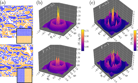
Figure 5. (a) System snapshots at  for high density particle configurations (ρ ≈ 0.4647 with simulation box size L × L with L = 520) from initially completely phase separated particle configurations shown in the insets. The systems are evolved under an applied force with F = 1.0 which breaks up the phase separated domains. (b) Averaged 'charge' structure factor
  in Fourier space shows two large central peaks corresponding to characteristic lengthscales forming due to the applied force F. At lower densities ρ ≈ 0.2065 (L = 780), the peaks form along the drive direction
  . Conversely, at larger densities ρ ≈ 0.4647
  in (c), the particle clusters elongate along the drive direction and the two central peaks in
  rotate to lie along the
  direction. Note that we also have rings around the peaks, which represent the average spacing of the particles. Various resonances at the higher densities in (c) indicate local crystallization, as seen in figure 1(d). Structure factors in (b, c) were averaged over a simulation time
  starting at
  .
.
Download figure:
Standard image High-resolution imageThe circular symmetry of our structure factors  is broken as the domains of A and B particles become anisotropic. In our simulations with F > 0, we average over the simulation trajectory from time
  to
to  , where we verify that the structure factor remains relatively time-independent. The averaged charge structure factors
  are shown in figures 5(b) and (c). We note two important differences compared to the F = 0 case: first, the peak at small
  is no longer symmetric. Instead of a ring, we find two peaks arranged either approximately parallel (figure 5(b) at low densities) or perpendicular (figure 5(c) at high densities) to the drive direction
  , depending on the force and particle density. Thus, we can no longer perform the circular average in q-space, as we did for F = 0. Second, the two peaks have a smaller amplitude for larger applied forces and do not grow with increasing time, indicating an arrested coarsening of the A and B colloidal domains. We will now study this more systematically.
We can check that the coarsening is indeed arrested by calculating  at different times t. To do this, we can take a slice through the q-plane that passes through the origin and the two central peaks in
  (shown in the lighter colors in panels of figures 5(b) and (c)). The results are shown in figure 6 for the larger colloidal particle density and a relatively small applied force F = 0.5. We see in figure 6(a) that the peaks at small values of
  fluctuate but remain at roughly the same positions, as seen more clearly in the inset. The full q dependence near these central peaks is shown for the earliest and latest times in figure 6(b). We see that, overall, the
  peaks near
  remain at well-defined positions for different times t. One can compare this behavior to the large difference at the earliest and latest times for the F = 0 case in figure 4(b). There, the peak at small
  continues to grow with time t and shifts rapidly toward smaller q (note the logarithmic scale). The peaks at
  in figure 6(a) do shift in time, moving toward larger
  values with increasing time. This corresponds to a decrease in inter-particle spacing, consistent with the formation of dense particle clusters (see figure 1(d)). The shift in the position of this peak can be compared to the position of the peak at
  in figure 4(b), which remains stationary in time. In other words, along with arresting the coarsening of A and B domains, the applied force generates a change in local particle densities, separating the system into regions of high and low colloidal particle density. We will explore this in more detail in the next section.
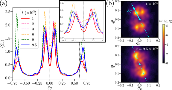
Figure 6. (a) Structure factor  averaged over a time interval
  , starting from the time t indicated. The particle density is ρ ≈ 0.4647 as in figure 4, but a force F = 0.5 is applied along the
  direction. We evaluate
  along a line that goes through the two central peaks at small
  (see top panel of figure 5(c)). The two thick red and blue solid lines show the structure factor at the earliest and latest simulation times, respectively. Note that the peaks at
  (shown in the inset in more detail) fluctuate but remain largely at the same positions. The peaks at larger
  shift toward larger
  at later times, corresponding to dense particle cluster formation. The thin dashed black lines indicate the
  values. (b) Color maps show the full
  dependence on q (for the earliest and latest times) and the line along which we measure
  for the plot in (a).
Download figure:
Standard image High-resolution imageHaving established that an applied force F arrests the coarsening of colloidal domains, we may look at the steady-state profiles of  by averaging over late simulation times t. The results for low and high particle densities are shown in figures 7(a) and (b), respectively, for varying applied force F, where we again evaluate the structure factors through a line that passes through the two central peaks (see right panels of figure 6). The application of a force at low densities decreases the characteristic domain size of the different colloidal species, as evidenced by the shifting of the central peaks toward larger
  values in figure 7(a). At larger colloidal particle densities, there is a similar shift which saturates at sufficiently large forces
  . These results are partially analogous to what is observed in a driven Widom–Rowlinson mixture (i.e. a binary mixture with short-range repulsive interactions) on a lattice, studied using Monte Carlo simulations in [18, 19]. However, on the lattice, the mixture (at sufficiently large particle densities) jams up into stripes of alternating
  and
and  particle domains, oriented perpendicular to the drive direction. The stripe size decreases with increasing drive magnitude. The precise reason for this stripe formation remains poorly understood. In our more realistic MD simulations described here, we do not find the ordered stripes. Instead, the domains of A and B particles reach a certain characteristic size depending on the magnitude of the force F. This size decreases with increasing F, much like the stripe width in the lattice simulations. The MD results are more reminiscent of the behavior of the lattice model at lower densities [19], where disordered clusters (instead of stripes) form, with a characteristic width along the drive direction. This characteristic width yields two peaks in the (charge) static structure factor
  . We also find these peaks in our MD simulations, although the peaks are not always aligned along the drive direction as they are in the lattice model case (see [19] for details). We shall now explore the peak position and orientation in more detail.

Figure 7. (a) Charge structure factor  averaged over simulation frames between times
  , evaluated along a line passing through the maximum values of
  near
near  , with
  the coordinate along the line, as illustrated in figure 6(b), for low particle densities (ρ ≈ 0.2065 and simulation box size L × L with L = 780). As the force F is increased, the two central peaks move toward higher q values. (b) At higher colloidal particle densities (ρ ≈ 0.4647 with L = 520), the two central peaks approach an approximately constant distance away from the origin in the q-plane as F is increased. The dashed lines indicate the position of the large
  peaks for F = 0 at
  , as in figure 4(b).
Download figure:
Standard image High-resolution imageWe show the positions  and orientations
  of the peaks in the structure factor
  in figure 8, where panel (a) illustrates these two features. The
  gives the distance between the origin in q space and the position of each peak (which are both equidistant from
  ). The angle
 ![$\theta_{\mathrm{max}}\in (-\pi/2,\pi/2]$](https://content.cld.iop.org/journals/1367-2630/25/3/033006/revision2/njpacb794ieqn175.gif) gives the orientation of the two peaks relative to the drive direction
gives the orientation of the two peaks relative to the drive direction  . In panel (b) of figure 8 we see that the peak positions at
  increase roughly linearly with the applied force F for low densities, while saturating to an approximately constant value for the higher colloidal particle densities. The low density results are analogous to those found for the lattice gas, where a disordered 'microemulsion' phase develops, characterized by two peaks in the static structure factor at positions
  (along the drive direction with
  ) [19].
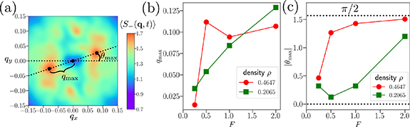
Figure 8. (a) Charge static structure factor shown for low particle density (as in figures 1(a), (b)) for F = 1, averaged as in figure 5. The two small  peaks are shown with black dots, including the distance from the origin
  and relative angle
  to the applied drive. (b) Peak distance
  away from the origin and (c) the angle
  of the peaks relative to the drive direction, computed for the low and high colloidal particle densities shown in figure 1 and averaged over simulation times
  . Note that as F is increased, the peaks move toward larger
  and rotate perpendicular to the drive direction
  .
.
Download figure:
Standard image High-resolution imageThe orientation of the peaks in  at small
  is subtle. We already observed in figure 5 that the orientation of the peaks can change depending on colloidal particle density. We also find that the magnitude of the force makes a difference. A larger force F > 1 rotates the peaks perpendicular to the drive direction (
 ). This is consistent with the formation of lanes of colloidal particles of opposite type forming parallel to the drive. Note that this behavior is in marked contrast to the lattice model results discussed in [19], where the peaks in
  always remain along the drive direction with
  . A more detailed analysis of the peak orientations is shown in figure 8(c). At smaller forces F and low colloidal particle densities, the orientation of the peaks is consistent with domains lying perpendicular to the drive direction,
  (green points in figure 8(c)). Conversely, at higher colloidal densities and large forces, the peaks are oriented perpendicular to the drive direction (
 ), corresponding to domains of A and B particles elongated along the drive direction (red points in figure 8(c)). Finally, note that although large particle densities ρ and large forces F both tend to orient the structure factor peaks perpendicular to the drive direction (
 ), increasing ρ can either increase or decrease
 (depending on the value of
  ), while increasing F tends to increase
  (because the force tends to break up the coarsening domains). Thus, the parameters
  and
and  play different roles.
It is interesting that our results here suggest that the orientation of the structure factor peaks depends on both the density ρ and the force F, by contrast to the lattice gas simulations in [18, 19] where the peaks are always displaced from the origin along the drive direction. We may speculate that the more realistic dynamics of our simulations here allow for the colloidal domains to rotate more freely, so that cluster formation is not locked into the drive direction as it is on the lattice. In addition, it is possible that the large particle density fluctuations play an important role, as the MD simulations exhibit very dense particle clusters, such as the locally crystalline patches shown in figure 1(d), which is not possible on the lattice. We also do not find ordered stripes at high densities, which robustly form in the lattice models [18, 19]. One possibility is that, at higher densities, the systems are kinetically arrested in our MD simulations, so that the ordered striped phases found in [18, 19] are restricted from developing.
4. Large density fluctuations
We now consider the overall distribution of the colloidal particles. As observed in figures 1(b) and (d), the applied force generates large density fluctuations and local regions with liquid-like and gas-like regions. At higher densities, the liquid-like regions generally move faster than the gas-like regions, which are hampered by more solvent particles, as shown in figure 3(b). These fluctuations can be quantified by calculating the probability P(N) of observing N particles in some circular 'window' placed at random in the simulation box. To calculate P(N), we generated 50 random points and counted the number of particles within a certain distance (the window radius) from each point, taking into account the periodic boundary conditions. We calculated histograms from these 50 points chosen for 2000 different frames at the latest times in the simulation, over a total time interval of  . Examples of the resulting distributions P(N) for a window radius of 40 are shown in figure 9(a) for the larger colloidal particle density ρ ≈ 0.4647 (see figures 1(c) and (d)) for different force values F. Note that applying a force F > 0 significantly changes the distribution: it widens and becomes asymmetric as the force generates large density fluctuations in the system. Systems with smaller particle densities, such as those in figures 1(a) and (b), also exhibit this broadening of the P(N) distribution, but only for a sufficiently large force F.
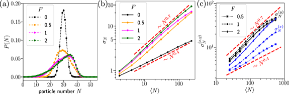
Figure 9. (a) Probability of observing N particles in a disc of radius 40 at late times for systems with colloidal particle density ρ ≈ 0.4647. The  case has a Gaussian distribution. For systems with an applied force F > 0, the distribution significantly broadens and becomes asymmetric (and non-Gaussian). A mean
  and standard deviation σN
can be calculated from these distributions. (b) The standard deviation σN
of the probability distributions P(N) for various window sizes from 10 to 110 (corresponding to different values of the mean
and standard deviation σN
can be calculated from these distributions. (b) The standard deviation σN
of the probability distributions P(N) for various window sizes from 10 to 110 (corresponding to different values of the mean  ). The red dashed lines indicate scalings ranging from a near-diffusive growth to a super-diffusive one for F > 0, indicating large density fluctuations. (c) Standard deviations of particle distributions as measured just along the drive (
 and perpendicular to the drive (
 ). The deviations
  (blue curves) and
  (black curves) are calculated by counting the number of particles in rectangles spanning the system in the perpendicular direction and then with some varying smaller size in the x and y directions, respectively. Note that we get much larger fluctuations perpendicular to the drive direction than along the drive [
 for a given
  ], demonstrating the anisotropy in the driven systems. This is consistent with the formation of dense 'lanes', seen in snapshots such as figures 1(d) and 5(a).
Download figure:
Standard image High-resolution imageThe density fluctuations can be further quantified by plotting the average  of each distribution P(N) versus the standard deviation σN
for a variety of window sizes. For equilibrium systems with a single phase and average particle separation, we would expect that
of each distribution P(N) versus the standard deviation σN
for a variety of window sizes. For equilibrium systems with a single phase and average particle separation, we would expect that  , in accordance with the central limit theorem. However, in a strongly driven system, we might expect long-range correlations to develop, generating giant density fluctuations which are characterized by
  with ν > 0.5. Such giant density fluctuations are a hallmark of active matter systems [34, 35]. We find an exponent ν ≈ 0.7 for our driven systems, as shown in figure 10(b). Note that a system undergoing a liquid-gas phase separation would also have particle density fluctuations consistent with ν = 1. Such a separation into dilute and dense regions occurs during mobility-induced phase separation (MIPS), the onset of which can often be interpreted as a liquid-gas transition [36]. A more thorough analysis would be required to see to what extent our system is similar to MIPS.
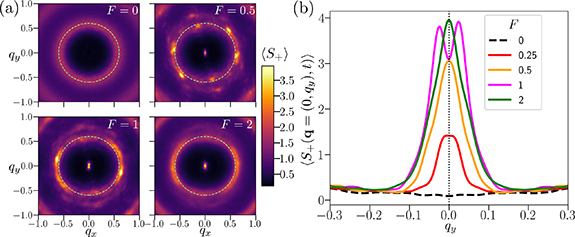
Figure 10. (a) Density static structure factors  (averaged over times
  ) evaluated at different values of the force F for the particle density ρ ≈ 0.4647 (simulation box size L × L with L = 520). When F = 0, we find a single ring at
  , corresponding to the average particle spacing λ ≈ 10.5 (see figure 4(b), also), which we have highlighted with a dashed light green circle, which we reproduce in the F > 0 panels for comparison. Note that the F > 0 cases also have a peak near
  . As the force increases, we get a larger contribution to
  along the drive direction (to the left and right of the ring). (b) Here we evaluate the structure factor through a vertical slice
  to observe the central peak in more detail. Note that the peak magnitude increases with F, with the peak completely disappearing for F = 0. This is an indication of the large-scale particle clustering for F > 0.
Download figure:
Standard image High-resolution imageOne way our system is clearly different from active matter and MIPS is that our particles are not self-propelled and we have strong anisotropies induced by the applied drive: The particles cluster more perpendicular to the drive direction (forming dense 'lanes'). This can be evaluated by looking at the standard deviations  along the two directions (the drive direction
  and the perpendicular direction
  ) separately. The deviations
  are measured by using long rectangular windows (spanning the system in the y and x direction, respectively) of different sizes. The results are shown in figure 9(c). Note that the blue curves, corresponding to particle density fluctuations
  along the drive direction, are smaller than the perpendicular fluctuations
  given by the black curves. At large force, however, we see large density fluctuations in both directions (solid lines in figure 9(c)).
The large density fluctuations are accompanied by changes in the density structure factor  . The results are shown in figure 10 for the large particle density case. The key feature corresponding to large-scale density fluctuations is the appearance of a sharp peak at
  in the presence of an applied force
  . Also, we find that at larger
  , the 'ring' corresponding to local particle arrangements (light green circle for the F = 0 panel in figure 10(a)) becomes deformed at larger forces F, with higher intensity along the drive direction. This can be seen by comparing the intensity maps around the light green circles in the panels of figure 10(a). Such an asymmetry indicates that the driven systems tend to have local particle arrangements with orientations sensitive to the drive direction. This can be seen in figure 1(d), where the small crystalline domains of different colloidal species are largely oriented such that rows of particles align along the drive. A similar result was found for the smaller particle densities at a sufficiently large force (see figure 1(b)).
For smaller particle densities such as those in figures 1(a) and (b), we also find a peak at  , but only for sufficiently large forces
  at which we observe the large density fluctuations. It appears that these fluctuations are accompanied by a redistribution of the solvent particles away from dense colloidal particle clusters, but a detailed analysis of this possibility would require more simulations at different solvent concentrations. The appearance of the
  peak in
  for applied drives is also found in the Monte Carlo simulations of the lattice gas model [19]. There, the peak appears even at small forces and particle densities. As mentioned previously, it is possible that our MD simulations have kinetic barriers which prevent the system from settling into certain non-equilibrium steady states. We thus might be prevented from seeing the development of the small
  peak at small forces and particle densities. We would expect the same to be true of experimental realizations of such driven systems.
5. Discussion and conclusion
In summary, we presented MD simulation results on a colloidal mixture of two particle types A and B with repulsive interactions, driven by a uniform applied field and immersed in a collection of solvent particles S. We found that the applied field generates two major effects: first, the coarsening of A and B particle domains (exhibited at zero force and sufficiently large colloidal particle density ρ) is arrested when the domains reach a certain characteristic size. Initially phase separated systems also break up into domains of this characteristic size. Second, the system exhibits large density fluctuations and separates into low density (gas-like) and high density (liquid-like or locally-crystalline) regions. These behaviors should be observable in an experimentally-realized colloidal system.
In addition, we verified that the coarsening at zero applied force (at sufficiently large ρ) is consistent with a conserved dynamics, where the characteristic domain size grows as  . We also found that the characteristic domain size at non-zero applied forces gets smaller with increasing applied force (especially at low particle densities), much like in a lattice model of the driven Widom–Rowlinson mixture [18, 19]. We also found that at high colloidal particle densities, the system forms lanes of dense, quickly moving particles parallel to the driven direction. Conversely, the driven Widom–Rowlinson lattice gas studied in [18, 19] jams up into ordered stripes perpendicular to the drive direction. The effects of the applied field on the particle distributions in our simulations were quantified by calculating the 'density' and 'charge' structure factors
  that take into account the overall particle positions and the relative distribution of the two colloidal species (A and B), respectively. It would be interesting to understand precisely why our simulations do not produce the ordered stripes (perpendicular to the drive direction) found in the lattice gas simulations in [18]. It is likely that the MD simulations presented here are prone to kinetic arrest (perhaps due to the formation of rigid, locally crystalline clusters), so that this kind of long-range ordering is prevented. We would expect to see similar behavior in experiments.
The low colloidal particle density results suggest that the non-equilibrium 'microemulsion' phase [19], characterized by two peaks in the 'charge' structure factor (indicating anisotropic domains with a characteristic 'width') and a single peak at  in the density structure factor, can be realized in realistic systems. A preliminary theory for such a non-equilibrium microemulsion phase, based on a lattice model, is presented in [19]. The basic idea is that charge and density fluctuations propagate at different velocities in the system due to the repulsive interactions between colloidal species. This velocity difference, when combined with thermal fluctuations, yields a peak in the (averaged) structure factor
  at a characteristic
  (along the drive direction
  ), with
  proportional to the drive strength. In our more realistic simulations, we find that the peaks in
  (and the corresponding anisotropic disordered domain geometries) may not always have a distinct relationship to the drive direction, with different orientations depending on the particle density and drive strength. Generally, we find that the domains are more elongated along the drive direction for increasing forces and densities. It would be interesting in future work to evaluate the dynamic charge/density structure factors for this model in order to see if there is a difference in the velocities and diffusivities of the charge and density fluctuations. This would require more robust statistics for our simulation runs, which may be computationally prohibitive. We expect that our work inspires such an endeavor in a real colloidal suspension.
Our results also illustrate the importance of the colloid-solvent interactions in these strongly driven systems. As a MD simulation integrates the equations of motion for each particle simultaneously, any uniform applied field with an implicit solvent (modeled by a Langevin thermostat, say) will simply uniformly accelerate all of the particles, with no effect on their relative dynamics or structure. Even introducing a large opposing friction force to mitigate the acceleration does not work because each particle will move with the same fixed velocity as set by the friction coefficient and applied force magnitude. Instead, here we have opted for a more computationally intensive approach and used an explicit solvent which does not experience the applied force directly. Collisions between colloid and solvent particles provide a friction for the colloids along the drive direction, without introducing an artificial, uniform velocity or acceleration. In addition, the choice of thermostat proved to be important: Our use of a Langevin thermostat for the solvent particles allowed for dissipation of the energy injected via the applied drive. Removing the thermostat or using momentum-conserving thermostats leads to acceleration of the entire system of colloids and solvents, preventing the establishment of a non-equilibrium steady state with a uniform average velocity.
There is clearly much more to explore in the future. We only considered a few simulation runs in detail, starting from either well-mixed or completely phase separated initial conditions. It would be important to check our results against larger system sizes and multiple runs. This would allow us to calculate more subtle statistical quantities, such as the dynamic structure factors. Given the similarities and differences between our results and the lattice simulations of a related system, it would be interesting to build an off-lattice Monte Carlo simulation to see if the ordered striped phases are possible. We did not observe them here, possibly due to kinetic arrest of the system into a more disordered phase. One potentially interesting avenue for future research would be to modify the initial conditions to see if striped phases could be stabilized under the applied drive.
Acknowledgments
MOL thanks R K P Zia, R Dickman, and I Schmidt for helpful discussions. MOL and DB are supported through the National Science Foundation, Division of Molecular and Cellular Biosciences (MCB), under Contract No. 2219289. Computational support was provided by the University of Tennessee. MD simulations research was supported by the Center for Nanophase Materials Sciences (CNMS), which is a US Department of Energy, Office of Science User Facility at Oak Ridge National Laboratory. This research used resources of the Oak Ridge Leadership Computing Facility (OLCF) at the Oak Ridge National Laboratory, which is supported by the Office of Science of the U.S. Department of Energy under Contract No. DE-AC05-00OR22725.
Data availability statement
The data that support the findings of this study are available upon reasonable request from the authors.
Appendix: Single colloidal species case
As a control, it is useful to see what happens when we consider a single colloidal species (particle A, say) in the presence of the solvent particles S. This is easily accomplished by removing the larger repulsion between A and B particles so that all the repulsive interactions become additive. In this case, as there is no difference between A and B particles, the only relevant structure factor is for the overall density,  . We may also calculate the particle clustering properties. The results are shown in figure 11.

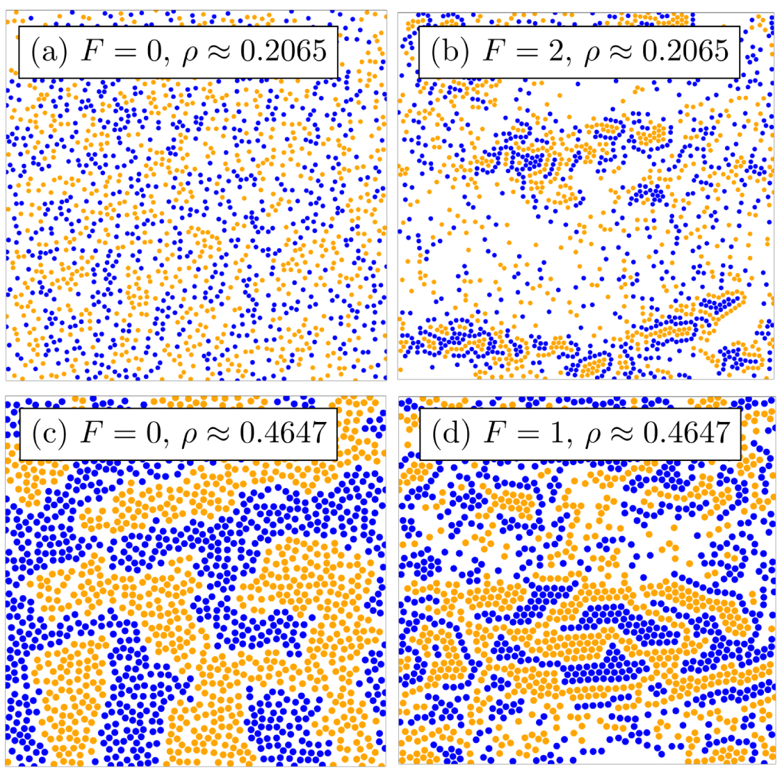
Figure 11. Particle clustering analysis for a system with a single colloidal particle type. (a) Particle distribution standard deviation σN
as a function of average particle number  in a given window, calculated for a system with colloid density ρ ≈ 0.4647. As for the binary mixture in figure 9(b), we find large density fluctuations at large applied forces F, but with an overall smaller magnitude. (b) The density static structure factor
  , averaged over simulation times
  , evaluated at
  . Note the development of a peak at small qy
with increasing force F. The inset shows the full q dependence for the F = 2 case. The black dashed line indicates the position of the ring for the F = 0 case. As in the binary mixture in figure 10(b), the applied force generates a large peak near
. Note the development of a peak at small qy
with increasing force F. The inset shows the full q dependence for the F = 2 case. The black dashed line indicates the position of the ring for the F = 0 case. As in the binary mixture in figure 10(b), the applied force generates a large peak near  .
.
Download figure:
Standard image High-resolution image
For the system with a single colloidal particle type, we find a similar increase in the particle distribution fluctuations σN
at non-zero forces F > 0 (figure 11(a)), and a corresponding development of a peak in  at
at  (figure 11(b)). Interestingly, the large
  behavior remains rotationally symmetric when a force is applied, with the outer 'ring' only inflating slightly compared to the F = 0 case, as can be seen by comparing the ring to the black dashed line in the inset of figure 11(b). The inflating ring suggests that there are more dense particle arrangements when the force is applied. However, unlike the case of the binary mixture of colloids, this system does not exhibit the localized crystallization and corresponding anisotropies in
  . Also, the standard deviations
  increase more graduatlly with the applied force
  in this single colloidal species case.