


Abstract
Synchronization of quantum nonlinear oscillators has attracted much attention recently. To characterize the quantum oscillatory dynamics, we recently proposed a fully quantum-mechanical definition of the asymptotic phase, which is a key quantity in the synchronization analysis of classical nonlinear oscillators (Kato and Nakao 2022 Chaos 32 063133). In this work, we further extend this theory and introduce multiple asymptotic phases using the eigenoperators of the adjoint Liouville superoperator of the quantum nonlinear oscillator associated with different fundamental frequencies. We analyze a quantum van der Pol oscillator with Kerr effect in the strong quantum regime and show that the system has several different fundamental frequencies. By introducing order parameters and power spectra in terms of the associated quantum asymptotic phases, we reveal that phase locking of the system with a harmonic drive at several different frequencies, an explicit quantum signature observed only in the strong quantum regime, can be interpreted as synchronization on a torus rather than a simple limit cycle.
Export citation and abstract BibTeX RIS

Original content from this work may be used under the terms of the Creative Commons Attribution 4.0 license. Any further distribution of this work must maintain attribution to the author(s) and the title of the work, journal citation and DOI.
1. Introduction
Spontaneous rhythmic oscillations and synchronization are phenomena ubiquitously observed in various fields of science and technology [1–6]. Owing to the recent progress in nanotechnology, synchronization in micro- and nano-scale devices has been realized experimentally [7–11] and experimental demonstrations of quantum phase synchronization in spin-1 atoms [12], in nuclear spin systems [13], and on the IBM Q system [14] have been reported. A number of theoretical investigations have also been performed to reveal novel quantum signatures in synchronization [15–47].
In the strong quantum regime where only a small number of energy states participate in the system dynamics, the discrete nature of the energy spectrum can give rise to explicit quantum signatures, such as multiple phase locking at several different frequencies [15] and synchronization blockade [16, 17]. In characterizing quantum synchronization, several definitions of the system's oscillation phase have been proposed [15, 18–22, 42–45].
In classical mechanics, nonlinear dissipative systems exhibiting spontaneous rhythmic dynamics can be modeled as limit-cycle oscillators. The asymptotic phase [1–5] is a fundamental quantity for the analysis of synchronization, which is defined by the oscillator's vector field and increasing with a constant frequency in the basin of the limit-cycle attractor. It provides the basis for phase reduction theory [1–6], a standard dimensionality-reduction method to derive phase equations describing weakly-coupled oscillators.
We recently introduced the asymptotic phase for quantum oscillatory systems [46] by extending the definition of the asymptotic phase for classical stochastic oscillatory systems [48] based on the Koopman operator theory [49]. This quantum asymptotic phase is defined fully quantum-mechanically in terms of the eigenoperator of the system's adjoint Liouville superoperator associated with the slowest decaying mode and hence applicable even in the strong quantum regimes where we cannot rely on the limit-cycle trajectory in the classical limit as in the semiclassical regime [26, 27, 50].
In this study, we further extend this definition and introduce multiple quantum asymptotic phases in terms of the eigenoperators with several different fundamental frequencies, i.e. with the eigenvalues possessing the smallest absolute imaginary part in the individual branches of the eigenvalues near the imaginary axis, which play dominant roles in synchronization dynamics. As an example, we analyze a quantum van der Pol oscillator with Kerr effect and show that it possesses several dominant eigenvalues with different fundamental frequencies in the strong quantum regime. By introducing the order parameters and power spectra in terms of the associated quantum asymptotic phases with respective fundamental frequencies, we reveal a torus-like structure of multiple-frequency phase locking of the system with a harmonic drive [15], which is observed only in the strong quantum regime.
2. Asymptotic phases for quantum oscillatory systems
In [46], we proposed a definition of the asymptotic phase for quantum oscillatory systems in terms of the eigenoperator of the adjoint Liouville superoperator associated with the slowest decaying mode, inspired by the definition of the asymptotic phase for classical stochastic oscillators [48, 49]. In this section, we briefly review this definition and extend it to introduce multiple quantum asymptotic phases by using the eigenoperators associated with several eigenvalues with different fundamental frequencies.
2.1. Quantum master equation
We consider a quantum nonlinear oscillatory system with a single degree of freedom coupled to reservoirs, and assume that the interactions of the system with the reservoirs are instantaneous and Markovian approximation can be employed. The time evolution of the system's density operator ρ is described by a quantum master equation [51, 52],
where  is a Liouville superoperator representing the evolution of ρ, H is a system Hamiltonian, Cj
is a coupling operator between the system and jth reservoir
is a Liouville superoperator representing the evolution of ρ, H is a system Hamiltonian, Cj
is a coupling operator between the system and jth reservoir  ,
, ![$[A,B] = AB-BA$](https://content.cld.iop.org/journals/1367-2630/25/2/023012/revision2/njpacb6e8ieqn3.gif) is the commutator,
is the commutator, ![$\mathcal{D}[C]\rho = C \rho C^{\dagger} - (\rho C^{\dagger} C + C^{\dagger} C \rho)/2$](https://content.cld.iop.org/journals/1367-2630/25/2/023012/revision2/njpacb6e8ieqn4.gif) is the Lindblad form (
is the Lindblad form ( denotes Hermitian conjugate), and the reduced Planck's constant is set as
  .
.
Introducing an inner product  of linear operators X and Y, we define the adjoint superoperator
  of
of  satisfying
  :
:
where ![$\mathcal{D}^{*}[C]X = C^{\dagger} X C - (X C^{\dagger} C + C^{\dagger} C X)/2$](https://content.cld.iop.org/journals/1367-2630/25/2/023012/revision2/njpacb6e8ieqn11.gif) is the adjoint Lindblad form. This
is the adjoint Lindblad form. This  describes the evolution of an observable F as:

In the Schrödinger picture, the density operator ρ evolves as in equation (1) while the observation operator F does not vary with time, and in the Heisenberg picture, F evolves as in equation (3) while ρ remains constant. The expectation value:

of F with respect to ρ is kept the same in both pictures (note that ρ is self-adjoint).
We assume that the Liouville superoperator  has a set of eigensystem (an eigenvalue and right and left eigenoperators)
  satisfying:

for  , where the overline indicates complex conjugate [53]. We also assume that among
  , one eigenvalue λ0 is always 0, which corresponds to the stationary state ρ0 of the system satisfying
  , and all other eigenvalues have negative real parts. This assumption also means that the system has no decoherence-free subspace [54]. Considering the system's oscillatory dynamics, we also assume that the eigenvalues of
  with the largest non-vanishing real part (i.e. with the slowest decay rate) are given by a complex-conjugate pair and denote them as Λ1 and
  , where
  gives the frequency of the slowest decay mode. One may also choose
  , which reverses the direction of the asymptotic phase. The sign of Ω1 can be chosen arbitrarily and will be fixed later.
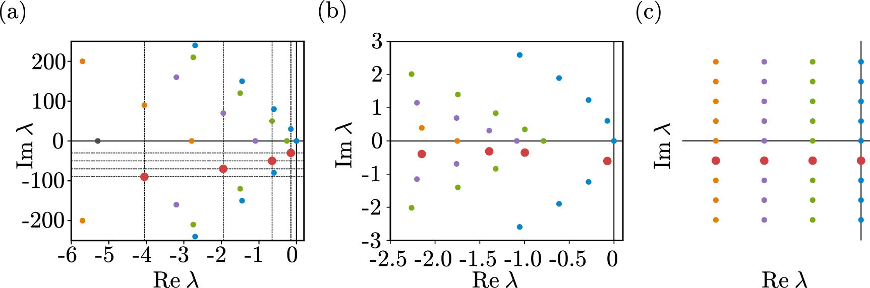
Figure 1 shows typical examples of the eigenvalues of  of the quantum vdP oscillator (see the next section for details). The eigenvalues form several branches. In the semiclassical regime (figure 1(b)), the rightmost branch is far apart from the other branches and thus it is the only dominant branch, while in the strong quantum regime (figure 1(a)), the branches are closer to each other and the system possess several comparably important branches. It can also be seen in the semiclassical regime (figure 1(b)) that the imaginary part of the eigenvalues are approximately integer multiples of the fundamental frequency (the smallest absolute imaginary part with the slowest decay rate) in each individual branch.

Figure 1. Eigenvalues of the Liouville superoperator  near the imaginary axis. (a) Strong quantum regime. (b) Semiclassical regime. The red dot on the light-blue branch represents the principal eigenvalue Λ1 with the slowest decay rate. (c) Classical limit (schematic). In (a)–(c), individual branches of eigenvalues are shown with different colors and the red dots represent the principal eigenvalues
  (
( from the right) with the fundamental frequencies in individual branches. In (a), the dotted lines indicate
  (
( ) in equation (18).
Download figure:
Standard image High-resolution image2.2. Phase-space representation
The density operator ρ can also be transformed into a quasiprobability distribution in the phase space [51, 52, 55]. We use the P-representation and describe ρ as:

where  is a coherent state specified by a complex value α, or equivalently by a complex vector
  ,
,  is a quasiprobability distribution of
α
,
is a quasiprobability distribution of
α
,  , and the integral is taken over the entire complex plane. The observable F is also transformed into a function in the phase space as:

where the operator F is arranged in the normal order [51, 52, 55]. By introducing the L2 inner product  of two functions
  and
and  , the expectation value of F with respect to ρ is expressed as:

The time evolution of  corresponding to equation (1) is described by a partial differential equation:

where the differential operator  satisfies
  . The explicit form of
  can be calculated from equation (1) by using the standard calculus for the phase-space representation [51, 52, 55]. The corresponding evolution of
  in the Heisenberg picture is given by:

where the differential operator  is the adjoint of
  with respect to the L2 inner product, i.e.
  , which satisfies
  .
.
The differential operator  also has a set of eigensystem (an eigenvalue and right and left eigenfunctions)
  which satisfies:

This eigensystem has a one-to-one correspondence with equation (5), where the eigenvalues  are the same as those of
  ; the eigenfunctions
  and
and  of
of  and
and  are related to the eigenoperators Uk
and Vk
of
are related to the eigenoperators Uk
and Vk
of  and
and  as:
as:

which follow from  and
and  .
.
2.3. Quantum asymptotic phase associated with the slowest decaying mode
In [46], we defined the quantum asymptotic phase function Φ1 of the system state ρ as the argument (polar angle) of the expectation of the eigenoperator V1 associated with the eigenvalue Λ1 satisfying  , namely,

We showed that this quantum asymptotic phase yields appropriate phase values, namely, it always increases with a constant frequency Ω1 as  with the evolution of ρ even in the strong quantum regime and reproduces the conventional asymptotic phase in the semiclassical regime [46]. We note that
  is not defined when
  .
.
This quantum asymptotic phase is a natural extension of the asymptotic phase for stochastic limit-cycle oscillators defined in terms of the slowest decaying eigenfunction of the backward Kolmogorov (Fokker–Planck) operator [48] from the Koopman operator viewpoint [49].
2.4. Multiple quantum asymptotic phases associated with different fundamental frequencies
In this study, we further extend the definition in the previous subsection and introduce multiple quantum asymptotic phases associated with several different fundamental frequencies by using the principal eigenvalues on different eigenvalue branches near the imaginary axis, and use them to characterize quantum signatures of synchronization in the strong quantum regime.
As shown in figure 1(a), in the strong quantum regime, multiple branches of the eigenvalues with different fundamental frequencies can exist near the imaginary axis, suggesting that not only the eigenvalue Λ1 on the rightmost branch but also the eigenvalues with the slowest decay rates on the other branches play important roles; for comparison, see figure 1(b) for a typical example of the eigenvalue Λ1 in the semiclassical regime, where only a single dominant branch of eigenvalues exist. We denote these eigenvalues by  and their imaginary parts, i.e. fundamental frequencies, by
  (
( ), and call
  the principal eigenvalues. Here, the first principal eigenvalue Λ1 and the fundamental frequency Ω1 are those introduced in the previous subsection. These principal eigenvalues on the individual branches are shown by red dots in figure 1(a).
In a similar manner to the phase function Φ1, we introduce the jth quantum asymptotic phase function  (
( ) of ρ as the argument of the P-representation of the eigenoperator
  associated with the principal eigenvalue
  satisfying
  , namely,

Note that  is not defined when
  . Since

we obtain  and therefore:

Thus,  always increases with a constant frequency
  with the evolution of ρ and plays the role of the asymptotic phase for any
It should be noted that  cannot be defined for the stationary state ρ0, because ρ0 is the eigenfunction of the Liouville superoperator
  with the eigenvalue
  and hence
  from the biorthogonality in equation (5). As will be shown later, for the stationary state of a periodically driven system,
  takes a non-zero value and the above definition of the phase functions can be used for the analysis of phase locking.
We stress that in the classical deterministic limit,  (
( ) is not independent from Φ1 and does not provide additional information, because
  (j ≠ 1) is equal to Ω1 according to the Koopman operator theory [56–59]. In the semiclassical regime,
  (j ≠ 1) differs only slightly from Ω1 as shown in figure 1(b) due to the effect of weak quantum noise and the corresponding decay rate for
  is much larger, so the corresponding mode does not play an important role. However, as we see in the next section,
  (
( ) is distinctly different from Φ1 and the corresponding decay rate characterized by
  (
( ) is comparable to
  in the strong quantum regime, hence the phase function
  (
( ) yields independent information from Φ1.
3. Quantum van der Pol oscillator with Kerr effect
3.1. Eigenvalues of the Liouville superoperator
As an example, we consider a quantum van der Pol oscillator with Kerr effect. The master equation is given by [15, 27, 46]:

where  , ω0 is the natural frequency of the oscillator, K is the Kerr parameter, and γ1 and γ2 are the decay rates for negative damping and nonlinear damping, respectively. We added a subscript 0 to the Liouville operator as we will introduce an additional external drive later.
We first consider a strong quantum regime with large γ2 and K, where only a small number of energy states participate in the system dynamics and the discrete nature of the energy spectrum plays important roles in the dynamics. We set the parameters as  and
and  , which are the same as in our previous study [46]. In the numerical calculation, we approximately truncated the density operator as a large-dimensional N × N matrix and mapped it into a N2-dimensional vector in the double-ket notation [60]. We can then represent the Liouville operator by a
  matrix and obtain the asymptotic phase in equation(13) from the eigensystem of this matrix [46].
Figure 1(a) shows the eigenvalues of  near the imaginary axis obtained numerically. We can identify several branches of the eigenvalues near the imaginary axis characterized by the principal eigenvalues
  whose fundamental frequencies
  are different from each other. Moreover, their decay rates, which are characterized by
  are comparable to each other. This indicates that not only the quantum asymptotic phase Φ1 associated with the principle eigenvalue Λ1 of the slowest decaying mode [46] but also those associated with the other principal eigenvalues
  can play important roles in the dynamics. We choose a negative value for each
  so that the corresponding
  increases from 0 to 2π in the counterclockwise direction.
In [15], it is shown that, in the strong quantum regime,  is an approximate eigenoperator of
  with the eigenvalue:

where  , namely,
  . As shown in figure 1(a), these eigenvalues correspond to the principal eigenvalues of
  , i.e.
  , and thus
  (
( ). This indicates that that periodic transitions between the adjacent discrete energy states play important roles in the oscillatory behavior in the strong quantum regime, where the differences in the transition frequencies arises due to the unequal spacing of the energy levels characterized by the Kerr parameter in equation (18).
As a comparison, we next consider the semiclassical regime where γ2 and K are sufficiently small and the semiclassical approximation can be taken [26]. We set the parameters as  and
and 
 , which are the same as those used in [46]. In this regime, we can approximate equation (9) by a quantum Fokker–Planck equation for
  and the system can be approximately described as a Stuart-Landau oscillator (Hopf normal form) subjected to small quantum noise [15, 27, 46]. (Therefore, the conventional quantum vdP oscillator is also called a quantum Stuart-Landau oscillator recently [36, 38] and a more appropriate model of the quantum van der Pol oscillator has also been proposed [38, 39].)
Figure 1(b) shows the eigenvalues of  near the imaginary axis, where the principal eigenvalues are shown by red dots on the individual branches;
  (
( ) is on the rightmost light-blue branch. In contrast to the strong quantum regime, the rightmost branch of the eigenvalues, approximately given by a parabola
  passing through
  , is isolated from other branches of eigenvalues with faster decay rates; the relative decay rate
  is more than three times larger than
  in the strong quantum regime in figure 1(a), indicating that only the rightmost branch is dominant in the semiclassical regime. Also, the fundamental frequencies of the other branches, defined as the smallest absolute imaginary part of the eigenvalues, are approximately equal to Ω1; the small differences in the fundamental frequencies arise from small quantum noise. Thus, it is sufficient to consider only Λ1 and introduce a single phase function Φ1 in this regime.
The system in the classical limit, i.e. in the limit of vanishing quantum noise, is described by the drift term of the approximate quantum Fokker–Planck equation for  , which represents the Stuart-Landau oscillator and possesses a stable limit-cycle solution [15, 27, 46]. Figure 1(c) shows a schematic diagram of the eigenvalues of the differential operator
  , which are equivalent to those of the backward Liouville operator
  , in the classical limit. They are given in the form
  , where κ1 is the real part of the largest negative eigenvalue and ω1 is the pure-imaginary eigenvalue with the smallest absolute imaginary part. Thus,
  (
( ) is identical to Φ1 and does not provide additional information, because
  (j ≠ 2) is identical to Ω1.
The above results suggest that the phase function  yields independent information from Φ1 only in the strong quantum regime. The existence of several dominant fundamental frequencies in the strong quantum regime suggests that the system behaves like a torus with multiple fundamental frequencies rather than a limit cycle with a single fundamental frequency, and that we need to consider the phase functions
  associated with
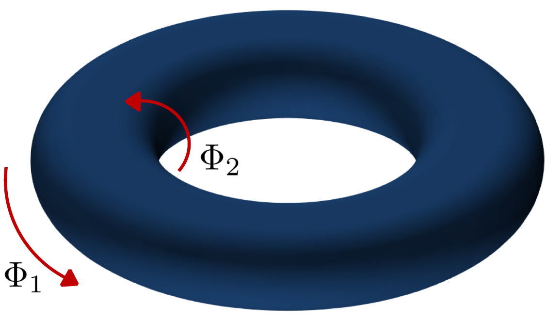
  in addition to Φ1 and Λ1. Figure 2 shows a schematic picture of the torus behavior of the system with two fundamental frequencies.

Figure 2. Schematic diagram of the torus behavior of the system with two fundamental frequencies.
Download figure:
Standard image High-resolution image3.2. Asymptotic phase functions in the strong quantum regime
In this subsection, we examine the validity of the quantum asymptotic phase functions in the strong quantum regime.
Figure 3 shows the asymptotic phase functions  for
for  and 4 of the pure coherent state
α
on the complex plane
and 4 of the pure coherent state
α
on the complex plane  . The parameters are the same as in figure 1(a). These asymptotic phase functions look similar, but they are associated with different fundamental frequencies and slightly different from each other near the origin as shown in the enlarged figures. Thus, they capture different oscillatory dynamics of the system. Though not shown, we may also draw similar asymptotic phase functions
  for
for  , which are less dominant. Here, the asymptotic phase functions for different values of j look similar to each other since they are identical in the classical limit [56–59], but the differences in their eigenfrequencies brought by the strong quantum effect take an important role in analyzing strong quantum signatures in synchronization.

Figure 3. Asymptotic phase functions of the quantum van der Pol oscillator with Kerr effect in the strong quantum regime. (a) Φ1, (b) Φ2, (c) Φ3, and (d) Φ4. The parameters are  and
and  . Figures in the bottom row show enlargements of the regions near the origin in the corresponding figures in the top row. In all figures,
  is chosen as the phase origin where
  (
( ).
).
Download figure:
Standard image High-resolution imageTo demonstrate that these quantum asymptotic phase functions yield appropriate phase values, we consider free oscillatory relaxation of ρ from a pure coherent initial state  with
with  at t = 0 and measured the evolution of the expectation values of Vj
and their arguments, i.e. their asymptotic phases
at t = 0 and measured the evolution of the expectation values of Vj
and their arguments, i.e. their asymptotic phases 
 , as well as those of the annihilation operator a for comparison. It is noted that, though the initial condition is a pure coherent state, the system state quickly becomes mixed due to the interaction with the reservoirs.
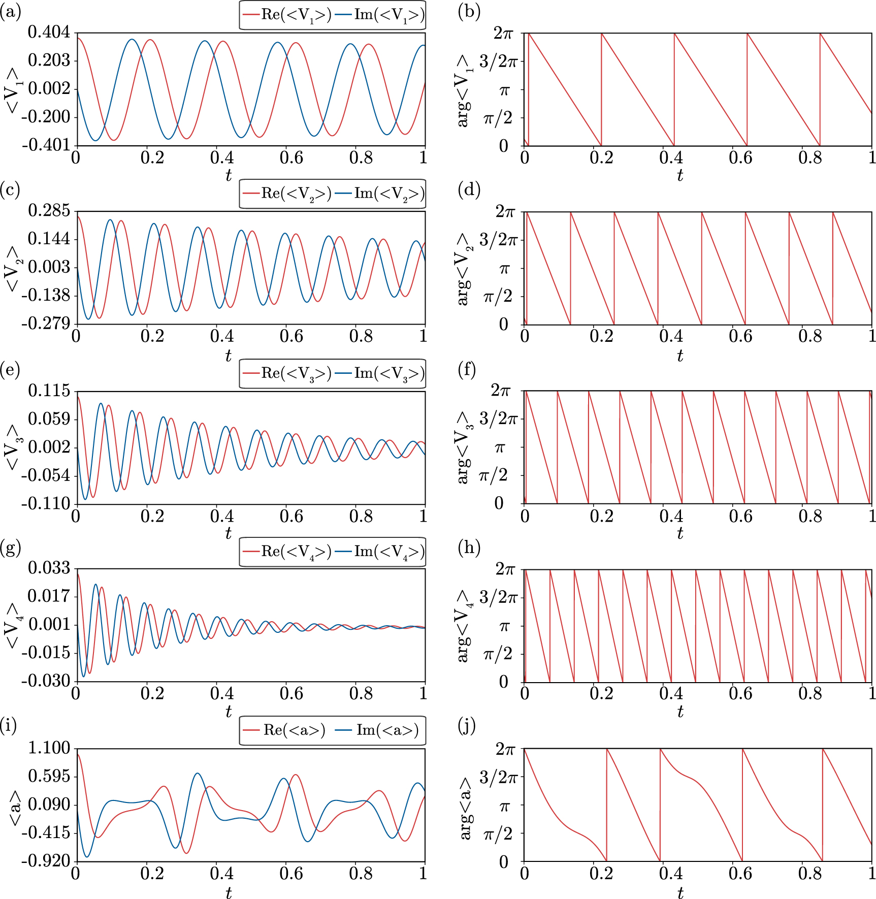
We can confirm that each  exhibits exponentially damped harmonic oscillations as shown in figures 4(a), (c), (e) and (g), and correspondingly, each
  gives constantly varying phase values with frequency
  as shown in figures 4(b), (d), (f) and (h), verifying the validity of the definition of the quantum asymptotic phases. It is noted that different asymptotic phases independently capture different oscillation modes in the evolution of ρ. In contrast,
  shown in figure 4(i) exhibits more complex oscillatory dynamics and the simple argument
  does not vary constantly with time as shown in figure 4(j). Thus,
  cannot be considered the asymptotic phase, although it is often used to define power spectra in the analysis of quantum synchronization. It is noted that the asymptotic phase is quantitatively different from the geometric angle also in the classical limit when the Kerr effect is added. In the strong quantum regime, due to the strong Kerr effect, the difference between the asymptotic phase
  and simple argument
  can be observed more clearly than in the semiclassical regime or in the classical limit [46].

Figure 4. Evolution of the expectation values of Vj
( ) and the annihilation operator a ((a), (c), (e), (g), (i)) and their arguments ((b), (d), (f), (h), (j)) from a pure coherent initial state in the strong quantum regime. The parameters are
  and
and  . (a), (c), (e), (g)
  , (b), (d), (f), (h)
  , (i)
, (i)  , (j)
, (j)  .
.
Download figure:
Standard image High-resolution image3.3. Revealing multiple phase-locking structure
We now analyze quantum synchronization of the vdP oscillator with a harmonic drive in the strong quantum regime using the proposed asymptotic phases.
The master equation in the rotating frame of the frequency ωd of the harmonic drive is:

where  is given by equation (17) with
  and the harmonic drive is represented by
 ![$\mathcal{L}_1 \rho = -i \left[ i E (a - a^{\dagger}),\rho\right],$](https://content.cld.iop.org/journals/1367-2630/25/2/023012/revision2/njpacb6e8ieqn167.gif) where
where  is the frequency detuning of the harmonic drive from the oscillator and E is the strength of the harmonic drive [15, 27, 46]. We use the same parameters as in figure 1(a) and vary the detuning parameter Δ by controlling ωd
while keeping the natural frequency ω0 fixed.
is the frequency detuning of the harmonic drive from the oscillator and E is the strength of the harmonic drive [15, 27, 46]. We use the same parameters as in figure 1(a) and vary the detuning parameter Δ by controlling ωd
while keeping the natural frequency ω0 fixed.
In [15], Lörch et al showed that this system under strong Kerr effect exhibits multiple phase locking to the harmonic drive at several detuning frequencies  (
( ), i.e. at
  , observed as multiple sharp Arnold tongues, while the corresponding classical system exhibits only a single broad Arnold tongue. It is stressed that K is the Kerr parameter, hence this is not the ordinary higher-harmonic phase locking at the frequencies
  with
with  (
( ); the multiple Arnold tongues are related to the periodic transitions between the adjacent discrete energy states. It is also noted that such multiple phase locking is robust to thermal noise under the finite temperature environment (see supplemental material in [15]).
In [15], the following order parameter Sa and power spectrum Pa defined using the annihilation operator a are used to analyze the system:


where the expectation is taken with respect to the steady-state density operator obtained from equation (19).
Here, in addition to these quantities, we introduce the order parameters and the power spectra in terms of the quantum asymptotic phases (or, more precisely, the corresponding principal Koopman eigenoperators) defined in this study. They are defined using the left eigenoperators Vj
of  as:
as:

where  and
and  (
( and 4). Here,
  and
and  quantify the phase coherence of the system, while θa
and θj
characterize the averaged phases of the system relative to the harmonic drive. We note here that we can use Vj
, which is defined in the original frame, in the rotating frame with the external drive since the eigenoperators Vj
changes only its phase factor by the coordinate rotation, i.e.
quantify the phase coherence of the system, while θa
and θj
characterize the averaged phases of the system relative to the harmonic drive. We note here that we can use Vj
, which is defined in the original frame, in the rotating frame with the external drive since the eigenoperators Vj
changes only its phase factor by the coordinate rotation, i.e.  with a constant Ω (see
  . Using these two quantities in equations (22) and (23), we can analyze both the phase coherence and frequency characteristics of the oscillator in quantum synchronization.
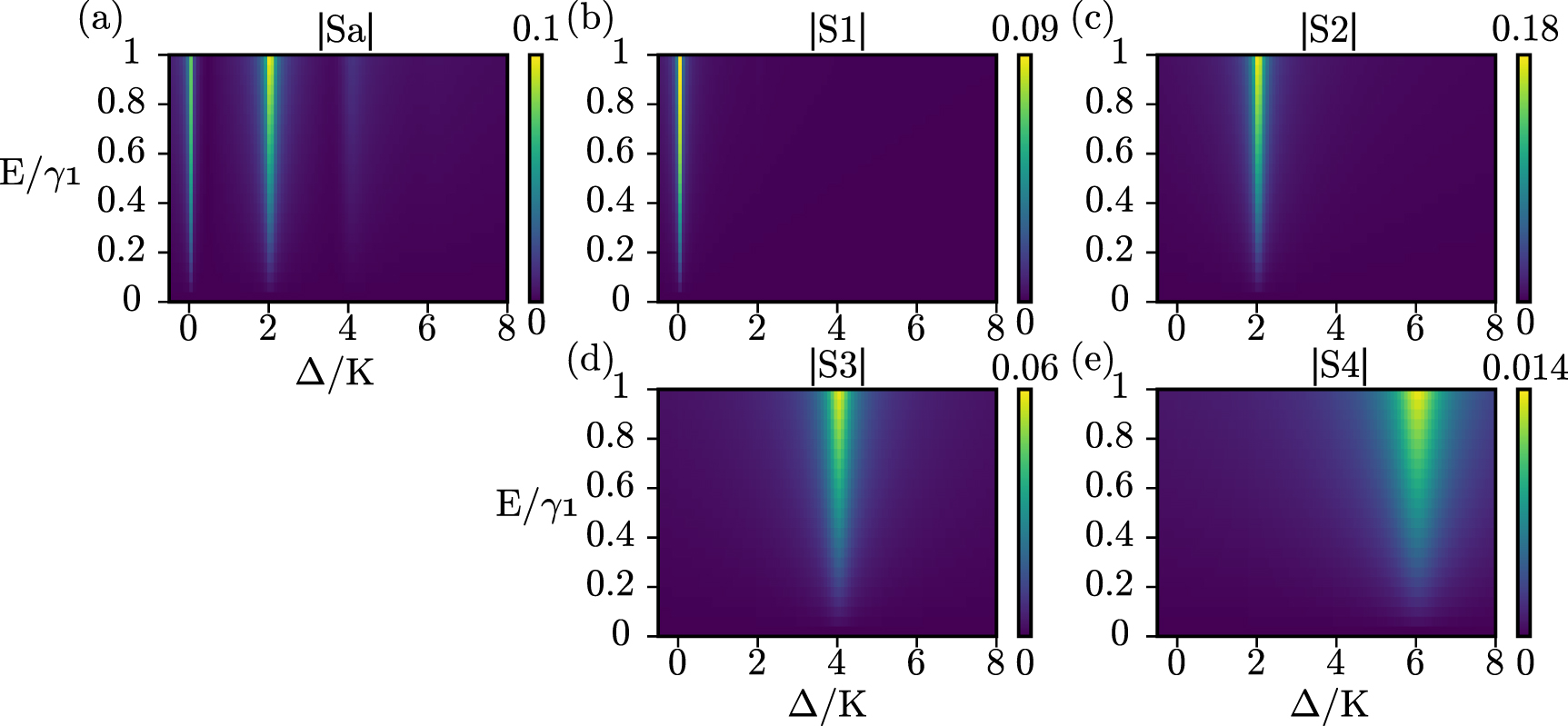
Figure 5 shows the dependence of the order parameters  and
and  on the detuning Δ and strength E of the harmonic drive. In figure 5(a) showing
  , several Arnold tongues representing phase locking of the oscillator at different frequencies are observed [15]. Figures 5(b)–(e) show
  for
for  and 4, respectively. It is remarkable that the Arnold tongues in figure 5(a) are clearly decomposed into individual Arnold tongues around
  in figures 5(b)–(e). This indicates that the order parameters in terms of the asymptotic phases can capture the phase locking dynamics at
  for different j individually.
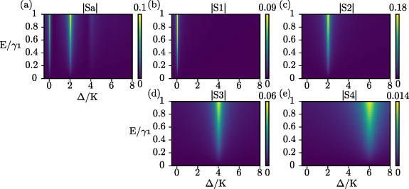
Figure 5. Dependence of the order parameters on the frequency detuning Δ (divided by K) and driving strength E (divided by γ1). (a)  . (b)–(e)
  . The parameters are
  and
and  .
.
Download figure:
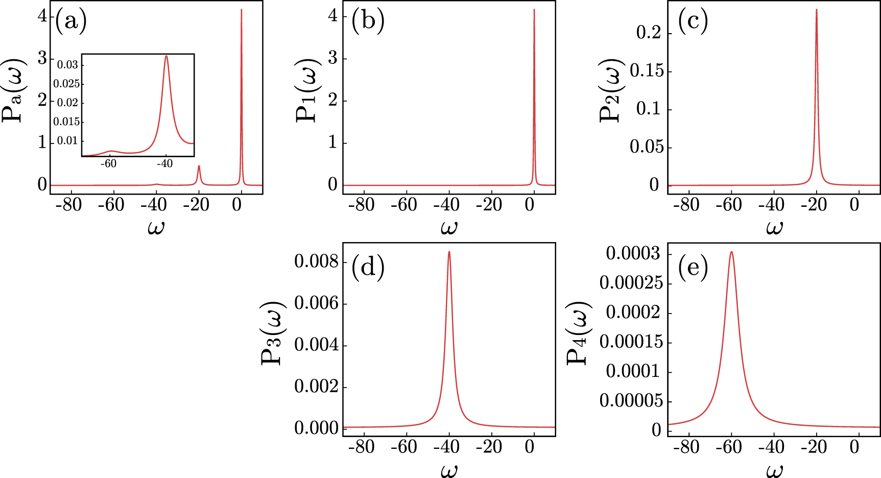
Standard image High-resolution imageSimilarly, figure 6 shows the power spectra Pa
and Pj
for  . Multiple peaks of Pa
in figure 6(a), which indicate multiple phase locking of the oscillator to the harmonic drive, are clearly decomposed into individual peaks around
. Multiple peaks of Pa
in figure 6(a), which indicate multiple phase locking of the oscillator to the harmonic drive, are clearly decomposed into individual peaks around  in figures 6(b)–(e) for Pj
(
in figures 6(b)–(e) for Pj
( , and 4). The Arnold tongue and power spectrum are sharper when the decay rate characterized by
  is smaller. Though not shown, we can also detect even smaller tongues and peaks with
  .
.
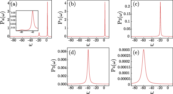
Figure 6. Power spectra. The parameters are  and
and  . (a) Pa
. (b)–(e)
. (a) Pa
. (b)–(e)  .
.
Download figure:
Standard image High-resolution imageThe above results reveal that, in the strong quantum regime, the system behaves like a torus with several fundamental frequencies and each of the associated oscillating mode individually exhibits phase locking to the harmonic drive at the respective frequency [61], resulting in the multiple Arnold tongues and spectral peaks. Such a torus-like behavior cannot be observed in the semiclassical regime where the system behaves like a noisy limit-cycle oscillator with a single fundamental frequency, because only the principal eigenvalue Λ1 is dominant. In contrast, in the strong quantum regime, due to the effect of quantum noise, visible differences between the imaginary part of the principal eigenvalues  (
( , and 4) arise and also the different branches of eigenvalues become closer to each other, resulting in the torus-like behavior.
4. Conclusion
In this study, we defined multiple quantum asymptotic phases of quantum nonlinear oscillators in terms of the eigenoperators of the adjoint Liouville superoperator associated with several fundamental frequencies from the Koopman operator viewpoint, which extends our previous definition of the quantum asymptotic phase associated with the slowest decaying mode of the system. We introduced the order parameters and power spectra in terms of the proposed quantum asymptotic phases and applied them to the analysis of a quantum van der Pol oscillator with Kerr effect. We successfully revealed that the multiple phase locking of the system with a harmonic drive at several different frequencies [15], which is an explicit quantum signature observed only in the strong quantum regime, can be interpreted as synchronization on a torus rather than on a simple limit cycle.
Though not discussed in this paper, it will also be interesting to introduce the amplitude functions in addition to the quantum asymptotic phases by extending the definition for classical stochastic oscillators [49, 62], which can be defined using the eigenfunctions associated with the eigenvalues on the real axis. The phase-amplitude description that uses both the phases and amplitudes may be applied to the analysis of quantum complete synchronization [18]. Also, investigating the mutual synchronization between two quantum nonlinear oscillators [16, 28, 47] by using quantum asymptotic phase functions is also a future work. We may be able to introduce a new measure for quantum synchronization between two oscillators, e.g. the normalized correlator [19], by using quantum asymptotic phase functions. It may be also interesting to extend our definition of the asymptotic phase for quantum synchronization in non-Markov open quantum systems [63].
We expect that the proposed definition of the quantum asymptotic phases will serve as a fundamental tool for analyzing strong quantum effects in synchronization [15, 16] and will be useful for future applications of quantum synchronization in the growing fields of quantum technologies.
Acknowledgments
Numerical simulations are performed by using QuTiP numerical toolbox [64, 65]. We acknowledge JSPS KAKENHI JPJSBP120202201, JP20J13778, JP22K14274, JP22K11919, JP22H00516, and JST CREST JP-MJCR1913 for financial support.
Data availability statement
The data that support the findings of this study are available upon reasonable request from the authors.


![$[a^{\dagger} a, V_{j}] = - k V_{j}$](https://content.cld.iop.org/journals/1367-2630/25/2/023012/revision2/njpacb6e8ieqn207.gif)

