


Abstract
We use the framework of sample space reducing (SSR) processes as an alternative to Boltzmann equation based approaches to derive the energy and velocity distribution functions of an inelastic gas in a box as an example of a dissipative, driven system. SSR processes do not assume molecular chaos and are characterized by a specific type of eigenvalue equation whose solutions represent stationary distribution functions. The equations incorporate the geometry of inelastic collisions and a driving mechanism in a transparent way. Energy is injected by boosting particles that hit the walls of the container to high energies. The numerical solution of the resulting equations yields approximate power laws over the entire energy region. The exponents decrease with the driving rate from about 2 to below 1.5 and depend on the coefficient of restitution. Results are confirmed with a molecular dynamics simulation in 3D with the same driving mechanism. The numerical solution of the resulting equations yields approximate power laws over the entire energy region. Deviations depend on the details of driving, density, and container.
Export citation and abstract BibTeX RIS

Original content from this work may be used under the terms of the Creative Commons Attribution 4.0 license. Any further distribution of this work must maintain attribution to the author(s) and the title of the work, journal citation and DOI.
1. Introduction
Driven dissipative systems remain a challenge for statistical physics for well more than a century. Even in their simplest form, such as an inelastic gas in a box with a simple driving mechanism that re-introduces dissipated energy during wall collisions, they have not been solved for stationary conditions. The equivalent of the Maxwell–Boltzmann distribution for elastic gases is still not fully known for inelastic gases. Much less is known for dissipative systems that abound in nature, including examples as diverse as non-equilibrium thermodynamics [1], granular matter, turbulent flow [2], self-organization [3], the earth [4], and living systems [5].
What has been understood in inelastic gases for several decades, however, is that due to the inelasticity in the collisions, generally, energy and velocity distributions are non-Maxwellian [6–9]. Contrary to the commonly considered system of inelastic granular gases with constant heating, leading to a stretched exponential steady state [10–12], some authors considered more extreme types of driving [13, 14] leading to power law velocity distributions. Since the 1970s, it was noted in many contributions in a wide range of fields that power laws play an important role. Power law solutions in the Boltzmann equation were found in numerous contributions [15–17]. Understanding the scaling velocity distributions in inelastic particle systems was pushed in the understanding of non-linear Boltzmann equations and the presence of multiscaling [14, 18, 19]. In the latter, power laws are derived analytically with an exponent that depends on the restitution coefficient,  , and the spatial dimension, D. This paper argues that besides the trivial solution for velocity distributions of inelastic gas particles where all particles are at rest, there exists a 'self-sustaining' solution, with power-law tails in the energy distribution, if dissipated energy gets re-injected at very high energies. The corresponding exponents,
  , for the non-trivial velocity distribution are computed, starting from a Boltzmann equation that implicitly relies on a weak molecular chaos assumption. The exponents depend on the dimension, the restitution coefficient, and the homogeneity index of the gas. The physical situation that we will analyze in this paper is similar to that of [14]. On the other hand, due to differences in the driving mechanisms the resulting power-law exponents in the tails differ considerably. Moreover, while the approach in [14] relies on the assumption of weak molecular chaos, here we suggest to use an entirely different approach to inelastic gases that is not based on the Boltzmann equation but on sample space reducing (SSR) processes [20], and compare the two approaches in the discussion. The main advantage of using the SSR approach is that, contrary to [14], no assumption of molecular chaos (even its weak form) is necessary. Moreover, we are able to calculate not only the behavior of the tail of the velocity distribution but we are able to get the shape of the entire distribution.
The SSR framework has been shown successful to deal with processes that violate detailed balance. We compute the energy (and velocity) distribution functions over the entire energy/velocity region for an inelastic gas in a box coupled to a simple driving mechanism, where energy is injected through those particles that hit the walls of the containing box. We understand the effects of the driving rate and particle density and check the analytical results with molecular dynamics (MD) simulations.
Driven systems are typically composed of a driving and a relaxation part, often in arbitrarily complicated ways. When systems relax toward lower (energy) states, this usually happens as an SSR process. The corresponding distribution functions are relatively easy to compute once the details of the driving process are specified [21]. For simple driving processes, SSR processes were found to exhibit universal power law statistics of visiting frequencies of the systems' states, regardless of the details in the relaxation dynamics.
1.1. Dissipative systems and the SSR argument
Dissipating processes such as inelastic collisions in a box are SSR processes in the following sense. Without driving, systems relax towards lower (energy) states over time. Assume that a system has M states that can be ordered or ranked (such as energy), labeled by  . The probability distributions of finding the system in (energy) state i are given by the eigenvalue equations of the following type,

where  is the transition probability that the system passes from state j to a lower state i. In the simplest case,
where the system jumps to any lower state with the weight, qi . It defines the probability of visiting state i. In the simplest case, whenever the lowest state is reached, the system is restarted at any randomly chosen energy level (driving process). Without driving, discrete SSR processes, despite being Markov processes, cannot run indefinitely since they reach a 'ground state'. The system cannot return to higher states, and the system is not ergodic in the sense of the Poincare recurrence theorem [22]. Adding a Markovian driving process to the system (e.g., coupling to energy source) that allows the system to revisit any state with a certain probability restores ergodicity in the Poincare sense. As a consequence, SSR processes with time-independent driving have a stationary state that is determined by the respective eigenfunction equation.
The solution to equation (1)—the distribution of visiting frequency—is an exact power law with exponent −1, sometimes referred to as Zipf's law,  , as long as the prior probabilities qi
are all equal or change polynomially, as iφ
with
, as long as the prior probabilities qi
are all equal or change polynomially, as iφ
with  ; see [20]. If the system is restarted before it reaches the ground state, say with probability
  (with
(with  ) at every timestep, the resulting distribution remains an exact power, however, now with exponent,
  . Remarkably, this is true for a huge class of choices of qi
, the result is always an exact power law [23]. Processes of this type are called SSR processes since, for the majority of the transitions, the number of reachable states (sample space) shrinks as the process unfolds.
. Remarkably, this is true for a huge class of choices of qi
, the result is always an exact power law [23]. Processes of this type are called SSR processes since, for the majority of the transitions, the number of reachable states (sample space) shrinks as the process unfolds.
Elastic collision processes (with energy conservation) can be described as SSR processes. For example, imagine a high-velocity particle with initial kinetic energy, E0, crashing into a box of resting classical particles all of the same mass that are sparsely distributed. When following the initial particle, after the first collision with a resting particle, it goes to a lower kinetic energy,  . The formerly resting particle now has kinetic energy and can kick other resting particles. For simplicity, we assume that it will never kick the initial particle again. The initial particle will lose energy along a sequence of n collisions, and we have an SSR process,
  . After some time, the initial particle will leave the box (no boundary). The system is driven by shooting particles with E0 into the box. The energy distribution of the particles can be computed analytically by solving the eigenvalue equation, which again yields an exact power law with exponent −2, see [24].
Note that inelastic two-particle collisions are exactly of SSR type, the total energy of both particles always being smaller after the collision. For the single test particle state, the exact SSR character of inelastic collisions is partly hidden by marginalizing the collision partner of the test particle, which, with some probability, can also increase its energy in a collision. Nonetheless, we can set up a Markov chain model for single particle transitions that includes the driving process and we expect to observe power laws in single particle energy distribution function with exponents close to −2 as solutions to the respective eigenfunction equation. However, the chain will be non-linear since marginalization of the test particle introduces a dependence of the single-particle energy transition probabilities on the 'ensemble of collision partners', i.e., the single particle energy distribution function. Here we show that the framework based on SSR processes also allows us to treat ensembles of inelastic collisions, in particular, the equivalent to the Maxwell–Boltzmann distribution for inelastic gases can be computed for the case of slow driving (many relaxation steps per driving events), which can be realized, e.g., by injecting energy when a particle hits the container walls. Note that in this way driving is not explicitly depending on the velocity of particles. Other models, such as [11], consider velocity-dependent driving (thermalization) and obtain stretched exponential velocity distributions. This situation can also be understood in the SSR framework if driving rates are state (i.e., velocity) dependent; see [21].
1.2. Inelastic particles in a box
We consider N identical classical particles with diameter, d, and unit mass, m = 1, in a 3D box of size L. Particles collide with each other inelastically with a coefficient of restitution,  . For the geometry of the collision, see figure 1(a). In the center-of-mass frame, two particles, 1 and 2, with incoming velocities v1 and v2, collide at an angle α. In this frame,
  , the relative distance vector is
  and the velocities after the collision are

 means elastic collision, for
  , kinetic energy is no-longer conserved,
  . Particles are reflected elastically at the walls of the box. The system dissipates energy in every particle–particle collision (except for exactly tangential hits).
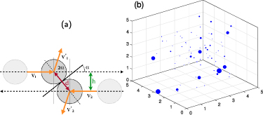
Figure 1. (a) Notation for the inelastic collision in the centre of mass frame. (b) Particles collide inelastically with each other in a box, walls reflect elastically. At the wall-collisions energy gets reintroduced with probability η to a fixed energy,  . The plot shows N = 125 particles after 10 000 collisions, their size represent their kinetic energy, d = 0.6,
  . Particles are not uniformly distributed within the box, slow ones lump together in a cluster.
Download figure:
Standard image High-resolution imageThere are many ways to re-introduce the dissipated energy to arrive at a stationary situation. In the spirit of an energy bath, the driving process could be realized such that particles that hit the wall are boosted to a high energy level, drawn from the driving distribution  (the wall has a temperature and transmits it to particles when in contact). Alternatively, randomly chosen particles could be injected with energy from the same distribution (for example, by shining laser pulses into the gas of particles). Many other possibilities can be imagined and implemented.
For the following analytical computations, we chose a driving scheme where particles, whenever they hit a wall, with a probability η are set to a fixed kinetic energy,  ; the direction of the particle left unchanged (up to reflection). In terms of velocity, a charging process for particle 1 means
  , where v is the unit velocity vector. The details of the driving process are known to be relevant for the resulting energy distribution functions, especially the driving rate plays a crucial role [21]. We define the driving rate, r, as the ratio of energy re-charging events per particle–particle collision. Note that r depends not only on η but also on the geometry of the system, in particular, the particle diameter and the particle density in the box.
Figure 1(b) shows a snapshot of an inelastic gas in a box. The size of the particles represents their kinetic energy. There is a cluster of low-energy particles at the lower right corner in the back of the box. Particles with high energy have a higher chance of getting re-charged in a wall collision.
2. Model
The idea is to compute the single-particle energy distribution,  , of a driven inelastic gas in a stationary state by solving an eigenvalue equation of the type given in equation (1), in particular

for a specific geometry of inelastic collisions.  is the stationary energy distribution function, and
  is the energy distribution of particles that just received energy from a driving event. Clearly, the stationary single-particle energy distribution,
  , resulting as a solution of this eigenfunction equation, also depends on
  , which we omit here for readability. Moreover, as described in detail in the SI, the single particle energy transition probability,
  , is defined by computing the energy transition probability of two colliding particles and then marginalizing to one particle—the collision partner—whose energy is drawn from the energy distribution,
  . It is thus clear that
  functionally depends on
  , which makes the eigenfunction equation non-linear in
  . We also do not indicate this functional dependence explicitly for the sake of readability.
The internal energy of the system is  , where
  and
and  denote the expectation values for the energy distribution and the driving energy distribution (energy source or bath). Per unit time, a fraction of ξ particles are drawn from
  and are replaced with a new energy drawn from
  . The other fraction of particles,
  , undergo particle–particle collisions and receive no energy charge from the source. Since we measure the driving rate, r, as the number of driving kicks per particle–particle collision, within a time span τ, where each of the N particles collides once on average, we get
  particle–particle collisions, and
  . τ is the average inter-particle collision time. Note that the driving rate, ξ, is defined as the number of driving events per particle per average inter-particle collision timespan, τ. Since τ depends on the average free path length and the average velocity, driving rates remain constant if we add particles while scaling the volume containing the particles such that the average free path length remains invariant and the average particle energy is kept constant. For constant volume and constant average particle energies, an increase of the particle density leads to an effective decrease of driving events per inter-particle collision time (if driving events per unit time are kept constant), proportional to the fraction of the average free path length involved.
To make sense of equation (3), note that if the two conditions that inter-collision times between particles are independent of particle energies (which they are not!) and that the gas is well-mixed would hold, then one could simply compute the energy transition probability distribution,  , as the energy transition probability of one particle involved in a collision. We obtain it from the energy transition probability of two colliding particles by introducing a test particle and integrating over the partner particle with the respective marginal energy probability distribution.
If the same conditions hold, then gas particles would further play the role of a particle ensemble, and the single-particle energy transition probability distribution could directly be used for the entire system, that is, the energy E in equation (3) would play a role of the state index, i, in equation (1).
However, particle inter-collision times are not independent of particle energies because, for a given average path length, the times between collisions behave as  , where E is the energy of the faster particle. More importantly, due to the inelastic nature of the collisions, fast particles will quickly lose energy in their collisions. It is fair to say that on average—within a given timespan between two driving events—it will be the fast particles that first dissipate their energy to the slow ones. Instead of trying to obtain exact results for the involved multi-particle collision process, we can reasonably approximate the true
  by breaking the symmetry between the test- and partner particle in the collision, assuming the partner particle is faster. For details and the derivation, see appendix
The single-particle transition probability in 3D, is obtained by integrating over the involved variables, ζ, α, and φ and their respective probability functions,  ,
,  , and
, and  (for the definitions, see appendix
  , with
  , and get

where  is fixed by the normalization condition,
  , the Heaviside function is defined as
  for x > 0, and
  , otherwise, and F is
with  . The term
  is introduced to account for the fact that the molecular chaos assumption is problematic for inelastic gases, energy equipartition is generally not realized [25] and, as discussed above, particle inter-collision times are dominated by the faster particles. For details, see appendix
3. Results
The self-consistent numerical solution to equation (3) with equation (4) is seen in figure 2(a) for different values of the internal energy, U. For details, see appendix  . For the numerical solution, we fix
  and U. The charging energy distribution is set to a delta function,
  , i.e. particles receive a fixed energy whenever charged. Clearly, the distribution is dominated by an approximate power law,
  , that extends over about two decades of E. We fit the corresponding exponents, β, with a maximum likelihood estimator within appropriate bounds [26] (the minimum energy for the power-law cutoff is chosen to be E = 2). Also, the driving peak at E = 5 is visible. For energies above 5, we see a much quicker drop in the energy distribution, a fact that has been described in [14]. These high-energy particles correspond to the relatively rare situation that a quick particle becomes faster in a collision.

Figure 2. Energy distribution of particles that collide inelastically, (a) as obtained from the numerical solution to equation (3) with equation (4) by fixing  and various levels of internal energy, U. Clearly an approximate power law decay is visible, as well as the driving peak at E = 5 that results from
  . U determines the driving rate, r. (b) Energy distribution as obtained from an MD simulation of an ensemble of 125 particles. The exponent of the power-law is β = 1.52. Inset: velocity distribution as obtained from the same MD simulation, also exhibiting a power law.
Download figure:
Standard image High-resolution imageFigure 2(b) shows the energy distribution,  , of the system as obtained from a straightforward MD simulation [27] of N = 125 particles with diameter d = 0.5 in a 3D box of size L = 5, and
  . To make the driving compatible with the analytical computation, particles that hit a wall were reset to a constant energy of 5 with a probability η = 0.5, which resulted in an observed driving rate of r = 0.006. For more details on the MD simulation, see appendix
  , very similar to panel (a). Also, the driving peak and the steep fall-off for higher energies is visible. It is also visible that for low energies, the energy distribution shows a deviation from the power law and forms a 'shoulder'. This is due to the geometric factors that are, of course, also present for elastic collisions. The MD simulation for
  is shown in blue and exactly follows the Maxwell–Boltzmann distribution (green),
  . The inset shows the velocity distribution,
  in red,
  in blue, green is
  . The fact that the blue and green lines practically coincide demonstrates the quality of the MD simulation.
In figure 3 we show the dependence of the exponent, β, that solves equation (3) as a function of the driving rate, r (red line), see appendix  , 0.8, and 0.9. The larger
  , the steeper exponents decline. Note that exponents are fitted to distributions like the one shown in figure 2(a) and thus contain an error of ±0.01 that is due to the fitting procedure [26]. The blue dots are the results from the MD simulations, that were realized by varying η from 0.02 to 1 in steps of 0.01. For each condition, ten independent runs of
  collisions were performed before fitting β. The spread in the simulation shows the variability and errors in the estimation of β. In every individual run, the driving rate was determined as the actual number of charging events per actual particle–particle collision. Generally, for 2D, we find qualitatively very similar results. We note a dependence of the exponents on geometrical parameters, such as the diameter, d, as we show in figure 4(a). Larger particles collide more often; thus the driving rate, r, decreases with increasing d, see figure 4(b). If one plots the exponent, β, versus r, the theoretical result (red line) holds, see figure 4(c). If we assume the existence of pure power laws between the 'shoulder' and the driving energy, the relation
  between the velocity and energy β exponents should hold, see appendix

Figure 3. Dependence of the power exponent, β, on the driving rate, r, for (a)  , (b)
, (b)  , and (c)
  . Red lines indicate the SSR results, i.e. the solution to equation (3). Dots show the MD simulation. In both cases, the exponents were fitted with a least likelihood estimator [26] within appropriate fit-ranges that are specific to the different
  . Note also that the lines have an error of about ±0.01 as a result of uncertainties in fitting.
Download figure:
Standard image High-resolution image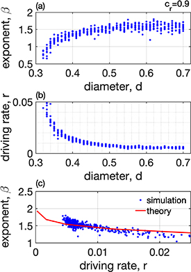
Figure 4. Dependence of the exponent on geometrical factors. (a) β, increases as a function of the diameter, d, however, the driving rate decreases as seen in (b), since particle–particle interactions become more frequent. Symbols show MD simulation results for  . (c) When the exponent is plotted against the respective driving rate we obtain the previous SSR result (red line). This confirms that the effect of particle size translates to the frequency of particle–particle collisions and the driving rate can be identified as the relevant parameter.
Download figure:
Standard image High-resolution image4. Discussion
We generalized the Maxwell–Boltzmann distribution for inelastic gases in their simplest form. We demonstrated that it is possible to derive the energy distribution for inelastic gases in the framework of SSR processes that are characterized by a specific type of eigenvalue equations that have been associated with universal power laws for slowly driven systems (SSR processes). We derived the corresponding eigenvalue equation that incorporates the collision geometry and a simple driving process, where particles are energized whenever they hit the walls of the box.
We demonstrate that the solutions to that equation (the energy distribution function) follow a power law for the high energy spectrum, whose exponents depend on the coefficient of restitution and the driving rate of the system. We confirm these findings with a straightforward MD simulation that leads to practically the same distributions in 3D. We checked that they remain valid also in 2D.
For dissipative systems, it is known that the energy distribution depends on details, such as the driving rate, density, possibly system boundaries, and the mode of driving. In our model, we used a type of driving that injects energy into single particles when they hit container walls. Other forms of driving, such as constant heating of particles, may lead to different velocity distributions [11, 12]. We checked numerically for the generality and robustness of the shown results with respect to these aspects. In the theory of SSR processes one knows that for slowly driven systems the driving rate is essential for determining the exponents of the energy distribution. We explicitly derived a theoretical relation of exponents and driving rates that is nicely confirmed with simulations. We confirmed that the effects on the exponents for different particle densities (that we implemented by varying the diameter of the particles, d) could be understood by relating density (more precisely the average free path length that depends on density and diameters) to driving rate. For the properly rescaled driving rates, we can predict the correct exponents again.
To understand the potential dependence of the exponents on the shape of the bounding container, we compared the energy and velocity distributions for simulations in a 3D regular box and a spherical boundary containing the same volume. We show the results in appendix
According to the theory of SSR processes, the nature of the driving process plays an important role in the distribution functions [21]. To understand its importance in relation to other influences, we implemented an alternative driving that injects the cumulative dissipated energy into particles that hit the wall. This means that at each of these energy injections, the total kinetic energy in the system is reset to its initial value. This allows for larger energy injections than the constant energy driving before, where particles were reset to a fixed energy of 5. Alternative driving is still a form of slow driving, meaning that, on average, there happen many more (dissipating) particle collisions than driving steps. In appendix
From these experiments, we conclude that there exist effects from driving rate, density, system boundaries, and the mode of driving. Our theoretical results allow us to understand those from the driving rate and density almost perfectly. Influences from boundary conditions matter to a very limited extent, and a more flexible driving mechanism leads to changes in the low-energy spectrum but leaves the power law tails of the distributions practically unchanged.
To compare our results with those of [14], note that the physical situation under consideration is comparable: the dissipative energy loss of the inelastic gas is re-injected (at a particular driving rate) through a few particles, i.e. some particles are reset to high energies, such that, on average, the gas maintains stationary internal energy. Where the approaches differ is in the way solutions are obtained. Ben-Naim and Machta [14] start from a Boltzmann equation with a 'homogeneity term'; we start by computing the pre- to post-collision single-particle transition probability of an inelastic gas by appropriately marginalizing the collision partner in a two-body collision. As a crucial element, we model the energy dependence of inter-particle collision times by explicitly breaking the symmetry between a test particle and a collision partner by assuming that the test particle is slower than the collision partner. This cannot be captured in the molecular chaos assumption. Then we solve a non-linear fixed point equation for the stationary particle energy distribution.
Our approach yields significantly smaller exponents than those reported in Ben-Naim and Machta [14], who report exponents of the velocity distribution in 3D in the range between −5 for  and −6 for
  , which translates to a respective exponent range for the energy distribution between −3 and −3.5. It is hard to pinpoint where exactly the differences in the exponents originate. One can only speculate that since in both approaches, exponents are sensitive to
  , the dimension (2D or 3D), and the driving rate, they will also be sensitive to the molecular chaos assumption being implemented or not. The latter is implemented in Ben-Naim and Machta [14] specifically, where high and low velocities get correlated. This is very different from what we do by effectively processing 'fast particles first?'. Phenomenologically, the exponents reported in Ben-Naim and Machta [14] more closely match the energy tails we observe above the driving energy, which include those fast particles that gain energy in collision processes. While the power-law behavior of the velocity distribution in Ben-Naim and Machta [14] is observed for large velocities, we observe the power-law decay of the velocity for a large range of velocities, which makes the result more plausible for applications to driven granular gasses.
The use of the Boltzmann equation might be problematic (even its non-linear version) since post-collision velocities cannot be considered independent. Instead, a large system of Bogoliubov–Born–Green–Kirkwood–Yvon (BBGKY) hierarchy equations should be used [29], for which moment closure obtained from the Boltzmann–Grad limit does not lead to a single Boltzmann equation. The presented alternative of the SSR approach overcomes the difficulty of solving the system of BBGKY hierarchy equations and offers a solution for all velocity scales. The present result is a clear demonstration that the SSR framework is powerful enough to compute energy and velocity distribution functions for particular driven dissipative systems, at least for relatively simple ones.
Acknowledgment
This work was supported in part by Austrian Science Fund FWF under P29032 and P33751, and the Austrian Science Promotion Agency, FFG Project under 873927.
Data availability statement
All data that support the findings of this study are included within the article (and any supplementary files).
Appendix A.: Derivation of the single-particle transition function
In the laboratory frame, the energies of two colliding particles are E1 and E2. We follow a reference particle 1 through the collision with energy E1 before and  after the collision. To see what happens to the particle we consider particle 2 with energy E2 drawn from the energy distribution
  of the gas. We now compute the transition probability
  .
.
 may depend on the reflection angle, 2α.
  is the ratio of the velocity before and after a collision in the centre of mass system, thus
  corresponds to the ratio of energies before and after a collision. In figure 1(a) (main text) it is easy to see that the tangent angle to the velocity vector, α, for the two colliding particles is
  , where h is the displacement between the particle centres orthogonal to the relative velocity. We assume that for inelastic collisions the reflection angle is 2α, as for the elastic case. However, there exists a monotonic function
  for
for ![$\alpha\in \left[0,\pi\right]$](https://content.cld.iop.org/journals/1367-2630/25/1/013014/revision2/njpacaf15ieqn89.gif) , that has a minimum for
, that has a minimum for  and
and  .
.  plays the role of an energy dissipation factor; it is a monotonic increasing function. A natural Ansatz is
  and
and  .
.
To compute the pair-energy distribution before and after a collision for the angle dependent  , one can proceed as follows. The energy of the particle-pair is given by
  . In centre of mass frame after the collision we have
  . In the laboratory frame this is
  , where the scalar product is
  .
. ![$\zeta\in[0,\pi]$](https://content.cld.iop.org/journals/1367-2630/25/1/013014/revision2/njpacaf15ieqn100.gif) is the angle between the velocity vectors. Since
is the angle between the velocity vectors. Since  ,
,  takes a maximum at
  , so that the maximal value of
  is
is  and it follows that
  . As a consequence, the range the values of
  are restricted to the interval
 ![$[c_\mathrm{r}^2 E_{12},E_{12}]$](https://content.cld.iop.org/journals/1367-2630/25/1/013014/revision2/njpacaf15ieqn108.gif) , i.e.
, i.e.  . Since the most likely value of
  is also where
  is maximal, we use the Ansatz
  , with
  .
.  , with the most likely value being at q = 1. We finally get
  , where the dependence on the particular initial kinetic energies is absorbed into the random variable q.
To compute the energy of one particle after the collision in 2D, we express it in terms of the prior energies, E1 and E2, the angle between velocities prior to the collision, ζ, and the reflection angle, 2α. Since we know how the total energy E12 behaves, we just have to calculate  after the collision. For this we rotate the laboratory coordinates such that v1 and v2 are in the xy-plane and the centre of mass velocity
  of particle 1 points in x direction. The velocity of the mass centre,
  , has an angle ζ with
  . For a picture of the geometry, see appendix B. We write

Using this Ansatz it follows that

and one arrives at

For 3D we introduce a rotation angle ![$\phi\in[0,\, \pi]$](https://content.cld.iop.org/journals/1367-2630/25/1/013014/revision2/njpacaf15ieqn120.gif) of the centre of mass velocity of particle 1 after the collision in the yz-plane, see appendix B, and get
of the centre of mass velocity of particle 1 after the collision in the yz-plane, see appendix B, and get

Next, we compute the distribution function of the reflection angle, 2α, assuming isotropic conditions. We need the probability of two colliding particles to be at an orthogonal distance, h. In 2D, all ![$h\in \left[0,D\right]$](https://content.cld.iop.org/journals/1367-2630/25/1/013014/revision2/njpacaf15ieqn121.gif) are equally likely, since there are just two possibilities (h and −h), and
are equally likely, since there are just two possibilities (h and −h), and  . In 3D,
  , since the area of collisions with orthogonal distance, h, is
  . To get the probability distribution for angle α,
  , one requires
  , and it follows that for 2D,
  and for 3D,
  . In 2D, half of the colliding particles are reflected with 2α, the other half is reflected at
  . In 3D, the collision plane can be rotated between 0 and 2π. Since the mirror reflection,
  , is not equivalent to the reflection with angle 2α, we extend the domain from
 ![$\alpha\in[0,\pi/2]$](https://content.cld.iop.org/journals/1367-2630/25/1/013014/revision2/njpacaf15ieqn131.gif) to
to ![$\alpha\in[0,\pi]$](https://content.cld.iop.org/journals/1367-2630/25/1/013014/revision2/njpacaf15ieqn132.gif) , with a respective renormalisation of the probabilities in
, with a respective renormalisation of the probabilities in  . To compute the distribution of angles between v1 and v2, under the assumption of isotropy, every angle, ζ, has only one possibility to be realized and the distribution is uniform,
  . In 3D, fixing v1, there is a rotational degree of freedom for v2 that has a fixed angle with v1, and
  . Finally, for the distribution of φ, that only exists in 3D, we safely assume it to be uniform in
 ![$[0,\pi]$](https://content.cld.iop.org/journals/1367-2630/25/1/013014/revision2/njpacaf15ieqn136.gif) , and
, and  .
.
Appendix B.: Geometry of the collision
For the computation of E1 in terms of the initial velocities, v1 and v2, the collision angle, 2α, and the angle ζ is depicted in figure 5.
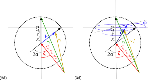
Figure 5. (a) Collision geometry in terms of velocities and angles for 2D. (b) Case for 3D with the additional angle φ.
Download figure:
Standard image High-resolution imageAppendix C.: Note on the molecular chaos assumption in dissipative systems
The molecular chaos assumption (that velocities of particles are well mixed) does not hold particularly well in inelastic collisions. It is well known that systems working irreversibly between an energy source and an energy sink can decrease their entropy, which in the simplest form is due to deviations from the uniform distribution of micro-states (equipartition property), caused by the energy current in the system. It is also known that non-equilibrium steady states have cycles (cycling theorems) and break local detailed balance, i.e. we cannot assume that the probability of observing two particles with velocities v1 and v2 together in a collision, factorizes into the marginal probabilities of observing v1 and v2 separately. In fact, if a particle receives an energy boost at the wall through the charging process, it has high energy (high velocity), and will quickly collide with a slower particle. Other slow particles can no-longer collide with this once high energy particle, since it already dissipated the energy to particles with typically lower energies. To assume the same free path-length—or alternatively, the same inter-particle collision times—for all particles is thus unrealistic. Slow particles will practically freeze out into clusters of slow particles, as observed in [6]. From time to time a high energy particle will hit such a cluster, and dissipate its energy to the cluster.
Appendix D.: Formula for the 2D single-particle transition probability

Appendix E.: Details on the numerical solution of the eigenvalue equation
To solve the equation numerically in reasonable time one must introduce a high energy cut-off and discretize the domains of the various integration variables in a relatively coarse way. For the solution, we chose to fix the internal energy U, that

where  , with
  , (all appropriately discretized). For the charging process we chose to re-introduce particles at a fixed energy, i.e. we set the energy distribution for the charging process to a Dirac-delta at E = 5, and get
  . Since U is fixed and
  is computed in the algorithm, by using equation (E1) we get the driving rate,
  .
.
The eigenvalue problem was performed in the following way. We appropriately discretised the integral domains of the angles. We bin the domains of the respective angles α, ζ, and φ into equal sized domains and use the bin-centres as the discrete angle values used in the sums approximating the integrals over the respective angles in the energy eigen-distribution equation. For α we use 13 bins, for ζ and φ 9 bins each. Using odd numbers of bins avoids the necessity of dealing with expressions of the form  in the formulas and the need for analysing and implementing the defined limits corresponding to the situation
  . The energy domain is more involved. First, we have to keep the number of bins low in order to respect constrains of computing time. At the same time, we would like to allow the internal energy, U, to be small, which implies that the bin-size for low energies needs to be small, and the high energy cut off,
  (remember
  ). We can accommodate all three criteria by using not equally spaced energy bins for the energy domain. We use N = 300 bins and place them in the following way

with a = 40 and γ chosen such that  .
.
The eigenfunction equation then is solved iteratively initialising the particle energy distribution function,  , uniformly distributed on the energy interval
 ![$\left[0,2U\right]$](https://content.cld.iop.org/journals/1367-2630/25/1/013014/revision2/njpacaf15ieqn149.gif) , and vanishing outside of it. The procedure converges quickly and we use a fixed number of seven iterations for obtaining our results, which we checked, is sufficient for our purposes. In each iteration we compute the energy transition distribution once. However, we iteratively update the energy distribution
, and vanishing outside of it. The procedure converges quickly and we use a fixed number of seven iterations for obtaining our results, which we checked, is sufficient for our purposes. In each iteration we compute the energy transition distribution once. However, we iteratively update the energy distribution  three times using the same energy transition probability so that we effectively iterate
  for
for  times for the solutions we obtain.
For computing the eigenfunction problem, we choose an energy threshold  and consider only energy bins below that threshold for the eigenfunction equation of the discretised distribution function
  . The energy bins
  n
between
n
between  and
and  are only used for estimating weight located in the tail of the distribution in order to minimise the deviation of energy expectation values induced by the energy cut off at
  , i.e. we approximate
  as a rectangular transition matrix
  with
with  and
and  . However, only the part
  and
and  is used for solving the eigenfunction problem. The remaining part of the matrix,
  and
and  is collected only for roughly estimating the tail of the energy distribution function,
  . The respective MATLAB codes are made available.
Appendix F.: Computer simulation of inelastic particles in a box
We use a standard MD scheme for spherical particles with diameter d in finite box of length L in one, two, and three spatial dimensions [27]. For simplicity, we set all masses equal, m = 1. Particles are initialized at random positions in the box with velocities in random directions. The absolute value of the initial velocity is taken from a uniformly distributed random number between 0 and 2. We distinguish between particle–particle collisions and particle–wall collisions. The update happens collision by collision. We compute the next particle–particle or particle–wall collision. For a particle–particle collision we update the velocities according to equation (2) in the main text, taking the coefficient of restitution into account. For a particle–wall collision particles are reflected off the wall as if it were an elastic collision, i.e. the directions after the wall collision are as for elastic reflections. For the base scenario with probability η we choose the particle for an energy update and set it to a fixed kinetic energy,  . After every update (particle–particle or particle–wall) the next collision is computed. The system typically converges to a reasonably steady (energy) state after a few thousand collisions, see figure 6. For the simulations we typically compute a few million collisions after removing the first 10 000 collisions.

Figure 6. (a) Total energy in the system as a function of collisions. Every 'time step' corresponds to one collision (particle–particle, or particle–wall collision). Wall collisions drive the energy up by a fixed amount, particle–particle collisions dissipate the energy. Steady state is reached after about 5000 collisions. (b) Situation for the alternative energy update, where the dissipated energy is re-introduced to particles such that the system gets back to its initial energy after every driving event.
Download figure:
Standard image High-resolution imageWe implemented an alternative energy update where energy is re-charged at wall hits with probability η, however, with exactly that energy that was lost in all the particle–particle collisions since the last charging process. In this way, the system is pushed back to its initial energy level after every recharging event. We found little effect in the distribution functions when using this alternative, see figure 7.

Figure 7. Distribution functions for the alternative driving scheme (red) still show extended power laws for (a) the velocity distribution, and (b) the energy distribution. Compare with figure 2 in the main text. Blue curves is MD simulation for elastic collisions,  , green is the exact Maxwell–Boltzmann result.
  .
.
Download figure:
Standard image High-resolution imageAppendix G.: Convolution product of power-laws—relation between β and γ
The convolution product,  , of power laws of type,
  , is written as

where the last factor does not depend on x. The value of the integral is practically insensitive to the value of x for  . A numerical analysis shows that the tail of the distribution follows a power law with the expected exponent,
  nicely if x0 is small (
 ). In other words, if x0 is small, indeed
  , with
  .
.
This means the following for the energy and velocity distributions,  and p(v). Assume that
  is an isotropic particle velocity distribution with
  . We use
  for the absolute value of the velocity vector;
  is the kinetic energy of the particles
By comparing terms in the transformation of variables we can identify
If we observe a power law  , then we necessarily observe a power law
  with
with  . Also
  holds.
Note that the relation between exponents β and γ is identical to the relation between a power law distribution (e.g. the one particle energy distribution function  ) and its convolution product with itself, the distribution function of two particles
  . That is, if
  it has the same exponent as

In figure 8 we see the realization of the expected relations between the two exponents, β from the energy and γ from the velocity distribution. The expected relation  is realized approximately in the numerical MD simulations.
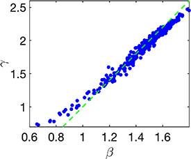
Figure 8.
β versus γ exponent , for the numerical MD runs shown in figure 4 in the main text. r = 0.9. The dashed green line indicates  . The deviations are due to the fact that we employ fixed fit-regions, which are not equally optimal for all values of d.
Download figure:
Standard image High-resolution imageAppendix H.: Situation with a different boundary
We perform the same simulation as in figure 2(b) and present the energy distribution in figure 9 as well as the velocity distribution in the inset, for two different boundaries: a 3D box (as in the main text) with box length, L, and in a sphere with the same volume with radius,  . The similarity is immediately visible, meaning that it is practically irrelevant if the container boundary is a box or a sphere. Of course, it cannot be ruled out that for other boundaries, the situation might be more involved, and the container boundary does play a role. Certainly, for strongly elongated boxes one would expect effects from effectively lower dimensionality, or when obstacles would be introduced into the volume, such as in Sinai billiard.
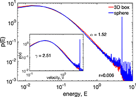
Figure 9. Distribution functions for the energy (main) and velocity (inset) for the 3D box boundary as in the main text (red) and for spherical boundary of the same volume. The difference in the distributions is almost negligible.
Download figure:
Standard image High-resolution imageFor the case of spherical boundaries, there exist situations where collective angular momentum builds up over many thousand energy injections. We subtracted the angular momentum of the system, whenever a threshold of  was exceeded (sum extends over all particles, i).
Appendix I.: Situation with a different driving mechanism
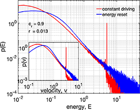
We perform a simulation with an alternative driving procedure and compare the resulting energy and velocity distributions (red) with those found in the driving with constant energy as in the main body of the work (red). The comparison is shown in figure 10 (velocity distribution in the inset). The alternative driving scenario works as follows: whenever a particle hits the wall with a fixed probability (that allows us to set a particular driving rate), the particle is given the cumulative dissipated kinetic energy since the last energy injection. In other words, we reset the total energy to the initial energy at every energy injection event. We set the driving rate that is approximately similar to the one used for the constant energy reset (ρ = 0.013). We use  . Note that this driving scenario cannot be described by equation (3) in the main text.
Figure 10. Distribution functions for the energy (main) and velocity (inset) for the driving scheme in the main text (red) and for the alternative driving, where the injected energy equals the cumulative dissipated energy since energy injection (blue). At every energy injection the total system energy is reset to the initial energy. Since the average energy for the alternative driving is higher the corresponding curve appears shifted to the right. The similarity in the tails of the distributions is remarkable.
Download figure:
Standard image High-resolution image
In figure 10 we see a very similar tail behaviour for the two driving schemes, both for the energy and velocity distributions. The low-energy shoulder is slightly different, mainly because the average energy in the two situations do not match (for the alternative driving, the energy is higher). The tail exponents almost perfectly match. Note that for the alternative driving the tails extend more towards high energies (because sometimes very high energies are injected). The reason behind the tail exponent being so similar can be understood by the theory of SSR processes, where the driving rate has been shown to determine power exponents. Both situations belong to what was referred to the 'slow driving' regime. In the slow driving limit, SSR predicts the same exponents [18].