


Abstract
We investigate two single-photon generation schemes and compare their suitability for use in time-bin entanglement encoding. A trapped ion coupled to an optical cavity produces single photons through a cavity-assisted Raman transition. By manipulating the phase relationship between time-bins of successive photons, distinct features in the interference pattern of a Hong–Ou–Mandel measurement emerge. Through careful selection of the initial state, detrimental effects of spontaneous emission can be significantly reduced. We demonstrate that this reduction allows us to impart a measurable phase profile onto the emitted photons making time-bin entanglement encoding feasible with an ion-cavity system.
Export citation and abstract BibTeX RIS

Original content from this work may be used under the terms of the Creative Commons Attribution 4.0 license. Any further distribution of this work must maintain attribution to the author(s) and the title of the work, journal citation and DOI.
1. Introduction
The controlled emission of single photons from a quantum system has many applications, from quantum key distribution [1–3] and quantum networking to distributed quantum computing [4]. For many of these applications, encoding the quantum information in the time domain instead of the photonic polarization is advantageous and opens new possibilities e.g. [5]. First demonstrated in 1999 [6], time-bin encoding offers protection against decoherence effects in optical fibers [7], which reduce fidelities and communication distances significantly; an example being polarization-mode dispersion [8] in polarization encoding. It has been shown that universal sets of quantum operations can be performed [9–11], reducing the complexity compared to other linear optical quantum computing schemes [12] and the storage of time-bin qubit in solids has been demonstrated [12].
The generation of time-bin encoded photons have been demonstrated with quantum dots [13, 14], parametric down conversion [15, 16] and proposed for atoms [17] but not with trapped ion systems.
Trapped ions coupled to optical cavities combine a highly controllable photonic interface with a quantum system that has long trapping and coherence times [18]. This facilitates the manipulation of the emitted photon's temporal and spectral properties [19, 20]. Single-photon emission with controlled frequency [21, 22], polarization [23], and temporal shape [19] has been demonstrated. However, while complete phase control of an emitted photon has been demonstrated in atom-cavity systems [24], it was previously beyond the capabilities of ion-cavity systems.
We demonstrate full control of an emitted photon's degrees of freedom, including its phase profile from an ion-cavity system. In particular, we show that this full control is possible even in weakly coupled systems. To demonstrate the phase control of the photons, we employ Hong–Ou–Mandel interference (HOM) in a similar manner to [24].
In the first part of this publication, we describe the experimental setup and how this is used to generate single photons in two distinct schemes. This is followed by the presentation of the results, their analysis and interpretation.
2. Setup
The setup, in which single trapped calcium ions are coupled to an optical cavity and serve as the laser controlled emitter of single photons is shown in figure 1 . A  ion is trapped in a linear Paul trap with an rf-electrode to trap center distance of 475 µm [25] and two axial dc endcap electrodes separated by 5 mm. At an rf frequency of 20.6 MHz. The rf trap drive amplitude and the dc voltage are chosen to result in secular frequencies in the radial and axial directions of 950 and 900 kHz respectively.
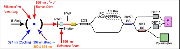
Figure 1. The experimental setup. The lasers involved in this experiment and their orientations relative to the cavity axis are depicted. A quarter-waveplate (QWP) and a polarizing beam splitter (PBS) filter the cavity emission by polarization. An 866 nm laser beam is optionally guided to the optical setup by releasing the shutter and moving a half-waveplate (HWP) into the beam path. The polarization in the delay arm is adjusted using the polarization controller paddles (PC). The electro-optical switch (EOS) guides the photons alternately into the delay and the direct arms, such that successive photons meet at the 50:50 beam splitter (BS). A time-to-digital converter (TDC) records the photon detection times on the detectors Det 1 and 2.
Download figure:
Standard image High-resolution imageThe optical Fabry-Pérot cavity is formed by a pair of highly reflective mirrors embedded in the endcaps along the trap axis. To prevent distortion of the trapping field, the mirrors are shielded by the endcap electrodes. The cavity length is 5.75 mm and the mirrors have a radius of curvature of 25.4 mm, leading to an ion-cavity coupling strength  MHz. The mirror transmissivities at 866 nm are 100 ppm for the output coupler and 5 ppm for the second mirror, which results in a cavity finesse of ∼60 000. In order to control the cavity frequency to better than 100 kHz, it is stabilized to a narrow-linewidth laser that in turn is referenced to the D1 line of cesium. This reference laser is sent through a fiber-coupled electro-optical phase modulator in order to add sidebands. For this a low frequency (10 MHz) rf signal from a function generator is added to the high frequency output (100s MHz) of a computer controlled rf synthesizer. This results in a comb-like spectrum of sidebands with a splitting of 100s MHz, all of which carry the low frequency modulation. The low-frequency modulation is used to generate an error signal via the Pound–Drever–Hall technique.
This error signal is sent via a proportional-integral circuit and a high voltage amplifier to a piezo actuator, which adjusts the cavity length. In this way the cavity frequency is stabilized to a high frequency side band of the reference laser.
By choosing the high-frequency modulation sideband order and adjusting its frequency with the rf synthesizer, the cavity frequency can be tuned over a wide range. The cavity is stabilized using the TEM70 mode, which in turn is tuned to overlap with the cavity resonance of the TEM00 mode of the single photon emission. The TEM70 mode has a small spatial overlap with the TEM00 mode, hence the light used to stabilize the cavity can be separated from the single-photon emission through spatial filtering. In order to align the quantization axis co-linear to the cavity axis and to split the Zeeman sublevels, the ion trap is in the center of a set of three Helmholtz coil pairs. The magnetic field is set to 0.5 mT.
The laser beams for cooling, state preparation, driving and re-pumping are frequency stabilized via a scanning cavity lock using the same reference laser as for the cavity stabilization [26]. The power, frequency and phase of all lasers are controlled via acousto-optical-modulators (AOMs).
In order to demonstrate the phase control over the photons emitted by the ion-cavity system, two consecutive photons, each with two time-bins, are generated. The first photon serves as a reference for the second photon in a HOM measurement. The two photons emitted by the system must arrive at the same time at a 50:50 beam splitter. To this end, the first photon is delayed by an optical delay line. This HOM interference setup is shown in figure 1. The cavity emission first passes through a quarter-waveplate to convert the circularly polarized photons to linear polarization. A polarizing beam splitter cube is then used to clean the polarization. It then passes through two shortpass filters to remove light that is used to stabilize the cavity length and is coupled into a single-mode polarization-maintaining fiber-coupled electro-optical switch (EOS) (Agiltron, NanoSpeed Ultra-Fast). The combination of stabilizing the cavity to the TEM70 mode and the shortpass filters reduce the amount of light of the reference laser that is coupled into the fiber to a level that is well below the single-photon detectors' dark count rate. The EOS directs the reference photons through a 1.5 km delay line fiber to one input port of a fiber-based 50:50 beam splitter (FBS). The second photon is directly led to the other port of the FBS by the EOS. The two output ports of the FBS are connected to superconducting-nanowire single photon detectors (Photonspot Inc.) with a rated quantum efficiency at 850 nm of 80%. A time-to-digital converter (TDC) (quTAU, qutools) records timestamps for each detection event. To measure the polarization distortion caused by the birefringence of the delay line fiber, a 99:1 beam splitter taps off 1% of the signal from one of the FBS outputs to a polarimeter. This distortion can then be minimized by polarization control paddles to match the polarization of the short path between the EOS and the 50:50 beam splitter. To measure the polarization change, an 866 nm laser is overlapped with the cavity emission and its polarization is matched to that of the single photons. The laser light is then directed either through the short or long arm of the interferometer and the polarization of the long arm is adjusted to match that of the short arm using the polarization control paddles. During the data taking the laser is blocked and the polarization matching is removed from the single photon beam path. The experiment is paused regularly (every ∼5 min) to measure and correct for the polarization distortion. To avoid coupling losses, all fiber-to-fiber connections in this setup are spliced.
3. Single photon generation schemes
We generate the single photons with two different schemes. The first scheme is depicted in figure 2 and is a modification of the scheme in [27], whereby a dual-drive cycle is employed.
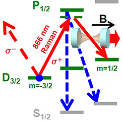
Figure 2. Scheme to generate single photons using a cavity-assisted Raman transition. The ion is initially prepared in the  state and is transferred to the
  level, while emitting a
  -polarized single photon into the cavity.
Download figure:
Standard image High-resolution imageThe ion is initially prepared in the  state via optical pumping. With the cavity coupled to the
  transition, the 866 nm laser on the
 transition drives a cavity-assisted Raman transition. This creates a σ−-polarized single photon in the cavity. The photon leaves predominantly through the output coupler and emerges at the cavity output. The ion-cavity system is in the weak coupling regime and, hence, the re-absorption of the cavity photon is strongly suppressed. The entire sequence to generate photons with the scheme is as follows (see figure 3). The ion is first Doppler cooled by a 397 nm laser for 1.5 µs while lasers at 850 and 854 nm repump the ion from the metastable states back into the cooling cycle (for details see e.g. [25]). The ion is then state prepared for 3.3 µs into the
  state using an 866 nm laser. To this end, a single laser beam at 866 nm containing σ− and π polarization components is applied. Repeated absorption and spontaneous emission cycles move the ion's
  state population to the
  level. A 397 nm laser pumps any population lost due to spontaneous emission back into the
  manifold.

Figure 3. Sequence to generate time-bin photons via a cavity-assisted Raman transition within the D level manifold. The lines represent the laser intensities for the different lasers. The cooling laser on the
  transition is blue, the re-pumpers during cooling are in brown and the laser for state preparation and pumping on the
  transition is red.
Download figure:
Standard image High-resolution imageThe single photon is then generated through a cavity-assisted Raman transition between the  and
and  states using a 866 nm laser beam aligned perpendicular to the cavity axis with linear polarization perpendicular to the B-field. In the ion's reference frame, the 866 nm drive beam alignment and polarization is seen as
  + σ− polarization. The cavity-assisted Raman transition takes 3.5 µs.
After the first photon is generated, the ion is again state prepared in the  state by optical pumping. The second photon is then generated with another drive laser pulse, however, halfway through photon generation, the phase of the AOM rf-drive can be switched, allowing us to arbitrarily select a phase difference for the second time-bin of the single photon. We forgo cooling the ion between photon generations to increase the amount of time available to state prepare the ion. To verify that this does not increase the ion temperature noticeably we perform an ion-temperature measurement with and without cooling between the photon generations. To this end, we translate the cavity with respect to the ion position and recorded the cavity-emission counts. Using the visibility of the cavity emission signal (see [25] for details) we confirmed that there is no noticeable temperature increase when removing the cooling between the photon generation intervals. The intensity of the drive laser for the cavity-assisted Raman transition is given a dual-Gaussian temporal shape, with a full width at half maximum (FWHM) of 700 ns and separated by 1.8 µs, measured using a fast photodetector. Amplitudes of the first and second peak are
  MHz and
  MHz respectively, blue detuned 24 MHz from resonance.
The temporal structure of the drive pulses is chosen to produce photons with equal probability of residing in the two time-bins and to maintain a reasonable emission efficiency within the constraints of the fiber delay line time limit. To this end, we experimentally optimized the timing as well as the intensity of the drive laser pulse. Initially, a numerical solutions of the master equation for an 8-level ion coupled to a cavity using QuTiP [28] was employed to optimize the efficiency and shape of the photons. The sequence was then implemented on the setup and the intensity of both drive pulses were iteratively tuned to deliver the highest efficiency with the correct photon population in both time bins.
While the first drive laser pulse intensity is optimized to transfer 50% of the ion's population into the  state, the second one is optimized to transfer the remaining population. Here the pulse intensity is a balance between the laser-induced ac-Stark shift and the increase in the effective Rabi frequency.
The temporal profile is produced by mixing the output of a function generator (Rigol DG4162) with the output of an rf synthesizer. In order to change the phase of the AOM rf-drive, the rf synthesizer phase is switched between the first and second time-bin drive pulses.
A small delay before and after photon generation is added to ensure all other lasers are switched off during the photon generation process. The overall probability of generation and detection of a single photon using this scheme is ∼0.061%. For comparison, we use a more conventional single photon generation scheme for  . In this scheme the single photons are produced by driving the Raman transition between the
  and
and  states. The scheme is depicted in figure 4. The ion is initially prepared via optical pumping in the
  state. With the cavity coupled to the
  transition, the laser at 397 nm on the
 transition drives a cavity-assisted Raman transition, which creates a
  -polarized single photon in the cavity. The entire sequence is shown in figure 5. After Doppler cooling, as in the previous scheme, the ion is prepared in the
  state by switching off the cooling 397 nm laser whilst leaving the repumpers at 850 and 854 nm on for
  s. The single photon is then generated through a cavity-assisted Raman transition between the
  and
and  states using a π-polarized 397 nm laser beam for 3.5 µs.

Figure 4. Scheme to generate time-bin photons via a cavity-assisted Raman transition from the  to the
  level. The ion is initially prepared in the
  state and is transferred to the
  level, while emitting a
  -polarized single photon into the cavity.
Download figure:
Standard image High-resolution image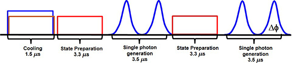
Figure 5. Sequence to generate time-bin photons via a cavity-assisted Raman transition from the  to the
  level. The lines represent the laser intensities for the different lasers. The cooling laser on the
  transition is blue, the re-pumpers during cooling are in brown and the laser for state preparation and pumping on the
  transition is red.
Download figure:
Standard image High-resolution imageThe intensity of this laser is given a dual Gaussian temporal shape, with 700 ns wide peaks (FWHM) and amplitudes of  MHz and
  MHz for the first and second peak respectively, red detuned 24 MHz from resonance. Similar to the scheme described above, these drive pulse parameters were chosen to produce photons with equal probability of residing in the two time-bins and to maintain a reasonable emission efficiency within the constraints of the fiber delay line limits. The overall probability of generation and detection of a single photon using this scheme is
  %.
%.
In order to calculate the photon correlations, we time stamp the photon arrival times using the TDC, gated to record only events within the time window in which the photons arrive at the beam splitter. Each photon detector is time stamped by a separate channel of the TDC and an additional electronic pulse is generated and time stamped every 256 cycles to synchronize the experimental sequence and the TDC. The temporal photon profiles extracted from the time stamp data for the two sequences are shown in figure 6. While the two peaks in the photon shape of the first sequence have the same width, the second peak of the photon shape in the second sequence is wider by about 150 ns compared to the first peak due to the different dynamics of the photon generation process. The profile for both sequences matches well with our numerical simulations apart from the earlier cutoff of the profile at around +1.5 µs due to the limited sequence length and the need for state preparation in the first sequence (see figure 6). This cut-off is not included in our simulation.

Figure 6. Temporal probability distribution of detecting single photon shown for the  scheme (top) and
  (bottom). To extract this plot, all the photon arrival times with respect to the sequence trigger during the measurements are sorted into 60 ns time-bins and the resulting histograms are normalized. The lines are obtained by numerical simulation.
Download figure:
Standard image High-resolution image4. Hong–Ou–Mandel measurements
The cross-correlation between the two detectors is obtained from the time stamp data and plotted in a histogram with a bin-width of 200 ns. For the  sequence 3302 476 photons were detected to produce the histogram with perpendicular polarization (fully distinguishable photons), 3430 821 photons were detected in order to measure the phase-flip interference and 1517 650 photons were detected to measure the interference with no phase-flip. Figure 7 shows the histograms of normalized detector coincidences with error bars representing the counting statistics errors. The solid lines are the numerical solutions of the master equation for an 8-level ion coupled to a cavity using QuTiP [28]. To obtain the expected HOM interference pattern, we calculate the first- and second-order coherence functions of the cavity emission [29]. The simulations are then scaled to fit the data. Noise and distinguishability due to imperfect state preparation has been included within the simulation.
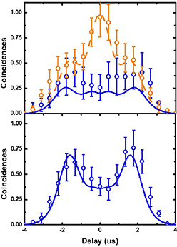
Figure 7. Hong–Ou–Mandel interference patterns for  scheme. Solid lines are obtained from numerical simulations of the system. Experimental data for parallel polarized photons, φ = 0 (top, blue) and
  (bottom, blue) is then scaled to the simulations and smoothed using an adjacent-averaging technique. Perpendicular polarized photons (top, orange dashed-line) are plotted for reference.
Download figure:
Standard image High-resolution imageFor completely distinguishable photons, the detector coincidences form a triple peak shape with the center peak being higher than the side peaks (orange data points in top graph in figure 7). The structure corresponds to the classical statistics of detecting the photons in either of the time-bins. This reference measurement is performed by rotating the polarization of photons through the delay fiber perpendicular to those from the direct path using the polarization controller, making the two photons distinguishable. For photons with optimized indistinguishability, the cross-correlations disappear as the two photons always emerge on the same output port of the beam splitter (blue data points in top of figure 7). However, the infidelity of the state preparation leads to an increase in the distinguishability of the photons and thus the increase in coincidences. The remaining population in the  state due to imperfect state preparation leads to an emission of a
  -polarized single photon during the single-photon generation interval. This is because the
  and the
 cavity-assisted Raman transitions are degenerate. Due to different Clebsch–Gordan coefficients of the transitions, however, the generated photons are not entirely indistinguishable. We take this in our simulations into account by having initial populations in the
  and
and  states. Due to the limited state preparation time within the constraints of the delay line length, we achieve only 85% state preparation fidelity. The structure of the measurement agrees well with the simulation, however, most data points are above the simulation. We suspect that the reason for this is the drift of the state preparation fidelity over the particularly long measurement time for this data set. Hence, we overestimate the average state preparation fidelity for our simulation over the entire measurement run. The blue trace and data set in the lower graph in figure 7 represents the case where a π phase-flip is applied between the two time-bins of the second photon. The data points agree well with the simulation. Here, the satellite peaks increase in size as shown in [24] as the photons are forced into opposite output ports of the 50:50 splitter, implying quasi-fermionic behavior. At the same time, the center peak disappears because the photons coalesce and emerge at the same beam splitter output if the photons are in the same time-bin and hence have the same phase. The appearance of the side peaks and the elimination of the center peak is a clear sign of the phase control we have achieved over the entire photon pulse.
In order to demonstrate the detrimental effect of atomic spontaneous decay on the control over the single photon emission process, we repeat the HOM measurements with the second scheme.
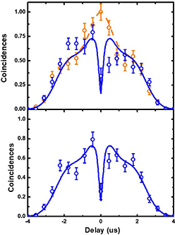
The cross-correlation of the two detectors is obtained in a histogram with bin width of 200 ns (see figure 8). 3956 791 photons were detected to make the fully distinguishable (perpendicular polarization) histogram, 3557 423 photons were detected to measure the interference with no phase-flip and 3627 794 photons were detected in order to measure the phase-flip interference. The error bars are the counting statistics errors. There is no significant statistical difference between the data with and without a phase-flip. This agrees with the simulations, which indicate there is no difference in the HOM interference for these two scenarios. The simulations are scaled to the data in the same way as before. The decreased visibility of the side peaks compared to the  sequence is a result of the larger peak width (see above).
Figure 8. Hong–Ou–Mandel interference patterns for  scheme. The data points show the experimental results for perpendicularly polarized photons (top, orange dashed-line), parallel polarized photons without phase-flip (top, blue) and with
  phase-flip (bottom, blue). The error bars are the counting statistics errors and the solid lines are the numerical simulations of the system.
Download figure:
Standard image High-resolution image
The similarity of the measurement with and without the phase-flip shows that the coherence time of the generated photons in this scheme is much shorter than the time-bin separation. During the pump laser pulse, there are several atomic spontaneous decay events on the  transition. Every decay event back into the
  manifold resets the cavity photon emission process. This results in any phase relation between time-bins being destroyed. For the
  scheme, the spontaneous emission of the
  level will, most likely (∼94%), leave the ion in the
  state, which is decoupled from the 866 nm drive laser. Hence photons cannot be produced once this has occurred and thus they maintain a phase relationship across time-bins.
5. Conclusion
In conclusion, we have demonstrated the full control of a time-bin qubit generated from an ion-cavity system. In addition to controlling the polarization and temporal profile, we have now demonstrated that phase control is possible by choosing the appropriate generation scheme. We have compared two schemes for generating single photons with a phase profile in an ion-cavity system. Due to spontaneous emission in the  scheme severely reducing the coherence length of the single photons, the phase relationship between time-bins is destroyed. Using the
 scheme, these scattering events are significantly reduced, allowing the single photon to remain coherent throughout its temporal length. This keeps the phase relationship between time-bins intact. With this improved photon generation scheme, the feasibility of time-bin encoding with an ion-cavity system has been demonstrated.
Acknowledgment
The authors would like to acknowledge funding by the EPSRC Hub in Quantum Computing and Simulation (EP/T001062/1).
Data availability statement
The data that support the findings of this study are available upon reasonable request from the authors.