


Abstract
Artificial spin ices (ASIs) are magnetic metamaterials comprising geometrically tiled strongly-interacting nanomagnets. There is significant interest in these systems spanning the fundamental physics of many-body systems to potential applications in neuromorphic computation, logic, and recently reconfigurable magnonics. Magnonics focused studies on ASI have to date have focused on the in-field GHz spin-wave response, convoluting effects from applied field, nanofabrication imperfections ('quenched disorder') and microstate-dependent dipolar field landscapes. Here, we investigate zero-field measurements of the spin-wave response and demonstrate its ability to provide a 'spectral fingerprint' of the system microstate. Removing applied field allows deconvolution of distinct contributions to reversal dynamics from the spin-wave spectra, directly measuring dipolar field strength and quenched disorder as well as net magnetisation. We demonstrate the efficacy and sensitivity of this approach by measuring ASI in three microstates with identical (zero) magnetisation, indistinguishable via magnetometry. The zero-field spin-wave response provides distinct spectral fingerprints of each state, allowing rapid, scaleable microstate readout. As artificial spin systems progress toward device implementation, zero-field functionality is crucial to minimize the power consumption associated with electromagnets. Several proposed hardware neuromorphic computation schemes hinge on leveraging dynamic measurement of ASI microstates to perform computation for which spectral fingerprinting provides a potential solution.
Export citation and abstract BibTeX RIS

Original content from this work may be used under the terms of the Creative Commons Attribution 4.0 licence. Any further distribution of this work must maintain attribution to the author(s) and the title of the work, journal citation and DOI.
1. Introduction
Artificial spin ice (ASI) are arrays of nanopatterned ferromagnetic arrays with frustrated inter-island dipolar interactions, leading to vastly degenerate low energy states. ASI systems were first intended as model systems mimicking magnetic frustration in rare-earth pyrochlores [1]. Scaling up atomic spins to 0.1–1 μm nanoislands allows system microstate readout using imaging techniques including magnetic force microscopy (MFM) [2]. Recently, ASI has found applications in novel computation [3–7] and reconfigurable magnonics [8, 9].
Ferromagnetic resonance (FMR) spectroscopy measures spin-wave spectra and has proved a potent tool for studying ASI based reconfigurable magnonic crystals [10–16]. In a seminal work, Gliga et al [10] predicted that FMR may be used for the quantitative detection of the population and separation of magnetic charge defects in square ASI. There is significant interest in using spin-wave spectra to identify ASI microstates [17], however, the majority of experimental ASI spin-wave studies focus on the in-field spectra, with only a few examples of measuring specific prepared states [18, 19]. Resonant mode frequencies are a function of the external, demagnetisation, and local dipolar fields, providing rich information via the spectral response to field [20–22]. A limitation of in-field FMR is that varying applied field Hext changes the spectra in multiple different ways. When Hext ∼ Hc (the array coercive field), the microstate evolves during reversal. In this field range the resonance frequency of any given mode changes due to increasing external field, changes in the demagnetizing field if the active island reverses and changes in the dipolar field landscape as neighbouring islands reverse. The precise microstate imprints subtle, informative details on the spin-wave spectra. However, these spectral shifts are dwarfed by mode frequency jumps associated with island reversal ( GHz vs 0.2 GHz) [19], limiting the microstate information revealed by field swept FMR.
Here, we employ zero-field FMR as a direct 'spectral fingerprint' readout of the microstate and nanoscale dipolar field texture. Removing the presence of external bias field, we can access fine microstate details across three ASI samples and deconvolute contributions to reversal dynamics arising from interisland dipolar interaction and the Gaussian distribution of coercive fields [23, 24] arising from nanofabrication imperfections termed quenched disorder. We extract absolute dipolar field magnitudes at specific lattice sites, challenging via alternative means. To illustrate the power of spectral fingerprinting and the additional information revealed versus magnetisation measurement, we prepare three distinct microstates with identical (zero) net magnetisation and observe starkly different spectra, giving rich microstate structure insight. These experiments demonstrate remanence FMR as a readout of both the microstate and nanoscale dipolar field texture at the nanoscale. This technique is widely applicable across a range of nanomagnetic systems [25–27] particularly in the nascent field of 3D artificial spin systems where direct microstate readout is extremely challenging [28–30].
Several proposed neuromorphic computation schemes [4–7] rely on measuring artificial spin system microstates as they shift in response to input stimulus. Currently, these schemes exist largely at the theoretical level due to a lack of reasonable means to measure the microstate—MFM is too slow, and PEEM and XMCD require unfeasibly large apparatus. Rapid, low-energy microstate-readout solutions are crucial to the progression of such neuromorphic computation hardware. The spectral fingerprinting approach described here is ideally matched to these tasks, with an experimental demonstration of ASI reservoir computation enabled FMR spectroscopy detailed in Gartside et al [31].
2. Methods
Remanence FMR functions by applying a microstate preparation field Hprep then removing it and measuring zero-field spectra. In zero external field Hext = 0 the Kittel equation gives a nanoisland resonant frequency f0:

where Hloc is the dipolar field from the surrounding bars,  ,
,  the local demagnetisation factors along and perpendicular to the field respectively, Nz
the out-of-plane demagnetisation factor, γ the gyromagnetic ratio (
the local demagnetisation factors along and perpendicular to the field respectively, Nz
the out-of-plane demagnetisation factor, γ the gyromagnetic ratio ( GHz/T for permalloy), μ0 the magnetic permeability of free space, and MS
the saturation magnetisation.
GHz/T for permalloy), μ0 the magnetic permeability of free space, and MS
the saturation magnetisation.
We consider three ASI samples, width-modified square (WM-S), figure 1(b), width-modified high-density square (WM-HDS), figure 1(c), and symmetric square (S-S) sample, figure 1(d) comprising identical bars. Width-modified samples allow for global field preparation of all four distinct vertex types (figures 1(e)–(h)) via an increase in width along a particular subset of bars, see supplementary information (https://stacks.iop.org/NJP/24/043017/mmedia) for MFM images of pure microstates. These samples allow us to demonstrate the spectral correspondence of remanence FMR when the microstate is well known, before using a range of disordered states in the S-S sample as a proving ground for spectral microstate fingerprinting.
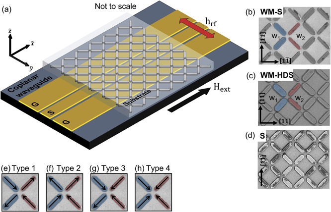
Figure 1. Experimental measurement schematic and samples description. (a) Schematic of flip-chip FMR measurement. The sample is mounted on the coplanar waveguide with the bar's long axis at 45 degrees to the external field Hext which is perpendicular to the microwave field hrf generated by the waveguide. Dimensions of ASI to waveguide not to scale. (b) and (c) SEM of WM-S and WM-HDS samples. WM-S bars are 830 nm × 230 nm (wide-bar w1)/145 nm (thin-bar w2) × 20 nm with 120 nm vertex gap (bar-end to vertex-centre). WM-HDS bars are 600 nm × 200 nm (wide-bar w1)/125 nm (thin-bar w2) 20 nm with 100 nm vertex gap. Where the ground state (GS) is accessible via mounting the sample along the [11] crystallographic direction and monopole state (MS) is accessible via mounting the sample along the ![$[1\bar{1}]$](https://content.cld.iop.org/journals/1367-2630/24/4/043017/revision2/njpac608bieqn5.gif) direction. (d) SEM of the symmetric square, S-S sample, bar dimensions 474 × 135 × 20 nm3, vertex gap 100 nm. It is mounted at 45 degrees to the bar's long axis or the [11] crystallographic direction. (e)–(h) Schematics of all four vertex types for a square lattice. Types 1, 2 are prepared by mounting the sample along the [11] direction and types 2, 3, 4 are prepared by mounting the sample along the
direction. (d) SEM of the symmetric square, S-S sample, bar dimensions 474 × 135 × 20 nm3, vertex gap 100 nm. It is mounted at 45 degrees to the bar's long axis or the [11] crystallographic direction. (e)–(h) Schematics of all four vertex types for a square lattice. Types 1, 2 are prepared by mounting the sample along the [11] direction and types 2, 3, 4 are prepared by mounting the sample along the ![$[1\bar{1}]$](https://content.cld.iop.org/journals/1367-2630/24/4/043017/revision2/njpac608bieqn6.gif) direction.
direction.
Download figure:
Standard image High-resolution image3. Results and discussion
3.1. Microstate control via width-modification
WM-S and WM-HDS samples, shown in figures 1(b) and (c) are square ASI with sublattices of wide (w1) and thin (w2) bars. Wider bars have lower coercivity (Hc1 < Hc2), allowing microstate control via the application of global field [19].
Mounting the width-modified samples along the crystallographic [11] axis and starting from a field saturated state type 2 (figure 1(f)) prepares a type 1 microstate (figure 1(g)) by applying a field such that only wide bars reverse. This is the system ground state (GS) [32–34] due to maximum dipolar flux closure, hence we term this field axis the 'GS' orientation. Rotating the samples and applying Hext along ![$[1\bar{1}]$](https://content.cld.iop.org/journals/1367-2630/24/4/043017/revision2/njpac608bieqn7.gif) direction (figures 1(a) and (b)) and reversing wide bars prepares the type 4 state (figure 1(h)), with 4 like polarity magnetic charges at each vertex. This results in highly unfavourable dipolar field interactions, termed the 'monopole state (MS)' [35–37]. We hence term this sample mounting the MS orientation. If there is any slight angular misalignment in the sample from the
direction (figures 1(a) and (b)) and reversing wide bars prepares the type 4 state (figure 1(h)), with 4 like polarity magnetic charges at each vertex. This results in highly unfavourable dipolar field interactions, termed the 'monopole state (MS)' [35–37]. We hence term this sample mounting the MS orientation. If there is any slight angular misalignment in the sample from the ![$[1\bar{1}]$](https://content.cld.iop.org/journals/1367-2630/24/4/043017/revision2/njpac608bieqn8.gif) direction, the MS orientation also prepares type 3 states (figure 1(g)) with 3 like polarity and 1 opposite polarity vertex charges.
direction, the MS orientation also prepares type 3 states (figure 1(g)) with 3 like polarity and 1 opposite polarity vertex charges.
MOKE hysteresis loops for WM samples are shown in figure 2(a)–(d). Figures 2(a) and (b) show the GS orientation WM-S (a) and WM-HDS (b) loops. Figures 2(c) and (d) show the monopole orientation WM-S (c) and WM-HDS (d) loops. The shape of the hysteresis loop changes significantly between the two orientations. The GS loops show two sharp steps in magnetisation at fields Hc1 and Hc2 corresponding to wide and thin bar reversal respectively. The magnetisation plateau between Hc1 and Hc2 corresponds to the type 1 state. MS hysteresis loops show gradual magnetisation reversal due to the energetically unfavourable dipolar field landscapes of type 3 and type 4 states. Here a clear plateau is absent, with kinks in the magnetisation curve revealing locations of the type 4 state in the WM-S sample (21 mT) and type 3 state in the WM-HDS (20 mT). The dipolar interaction in the WM-HDS sample is too strong for a pure type 4 state to be observed.
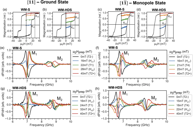
Figure 2. Microstate control via width-modification and corresponding remanent spectra. (a)–(d) MOKE hysteresis loops in the GS orientation for the WM-S (a) and the WM-HDS (b) sample. Hysteresis-loops in the MS orientation for the WM-S (c) and the WM-HDS (d) sample. Colour coded remanence magnetisation curves from the same preparation field as the spectra in (e)–(h) are also shown. (e)–(h) Differential remanence FMR spectra for WM-S sample in GS (e) and MS (f) orientations and WM-HDS sample in GS (g) and MS (h) orientations. GS-orientation spectra corresponding to preparation fields for the type 2− (black), Hc1 (blue), type 1 (green), Hc2 (orange), type 2+ (red) microstates. In the MS orientation the spectra shown correspond to the type 2− (black), Hc1 (blue), type 3/4 (green), Hc2 (orange), type 2+ (red) microstates.
Download figure:
Standard image High-resolution imageThe remanence traces on the MOKE loops (coloured lines) leading from the major loop back to zero-field, showing the resultant magnetisation after the microstate preparation protocols. Figures 2(e)–(h) show remanence FMR spectra corresponding to microstates prepared by the remanence traces shown in figures 2(a)–(d). The spectral plots show two major absorption peaks at  GHz and
  GHz corresponding to bulk centre-localized modes in wide (M1) and thin (M2) bars respectively. Spectra shown in figures 2(e)–(h) exhibit characteristic changes in the peak profiles of M1 and M2, both in terms of resonant frequency f0 and differential amplitude
  depending on the microstate.
3.2. Ground state orientation remanence FMR
With Hext along the [11] orientation, samples were saturated into the type 2− state by applying an initial −200 mT field. The preparation field Hprep was then stepped from 0–40 mT in 1 mT steps, measuring zero-field spectra after each field. Figures 3(a) and (b) show differential spectral heatmaps of the preparation field against FMR frequency. When wide bars reverse at Hc1, the sample switches from the type 2− to the type 1 state. Thin bars reverse at Hc2, switching from the type 1 to the type 2+ state. Due to the stable energetics of the type 1 GS, Hc2 is increased in this configuration relative to an isolated thin bar, broadening the type 1 field window.

Figure 3. GS orientation Remanence FMR and microstate evolution. (a) and (b) Heatmap of differential FMR amplitude as a function of frequency at a range of preparation fields Hprep in the GS orientation for WM-S (a) and WM-HDS (b) samples. Magnetisation schematics of the type 2−/type 1/type 2+ microstate trajectory are shown in (c). (d) and (e) Extracted resonant frequencies f0 for the bar-centre localized modes are shown on scatter plots in blue (wide) and red (thin) for WM-S (d) and WM-HDS (e). Samples were initially saturated in −200 mT before a preparation field Hprep was applied in a positive direction and the FMR spectra were measured in zero-field. This was repeated for Hprep in 1 mT steps from 0–40 mT. Coercive fields are marked Hc1 (wide bar) and Hc2 (thin), accompanied by a phase reversal of the relevant mode in the differential plot. (f) and (g) MOKE measured remanence magnetisation (black trace, left y-axis) and FMR amplitude of the M1 (blue trace, right y-axis) and M2 (red trace, right y-axis) modes for WM-S (f) and WM-HDS (g).
Download figure:
Standard image High-resolution imageAs the sample enters a type 1 state the local dipolar field landscape shifts, blueshifting both modes in figures 3(d) and (e). M1 blueshifts by 60 ± 7 MHz (WM-S) and 70 ± 5 MHz (WM-HDS) while M2 blueshifts 46 ± 8 MHz (WM-S) and 111 ± 8 MHz (WM-HDS). Due to the smaller lattice parameter and larger dipolar field of WM-HDS, frequency shifts are enhanced relative to the WM-S sample. Similarly, this explains the relative difference in shift magnitude between M1 and M2. The dipolar field emanating from the wide bar is stronger due to its larger volume, so it induces a greater frequency shift on the thin bar, while the frequency shift in the M1 mode is smaller.
Fitting the in-field FMR response with the Kittel equation to M1 and M2 modes, we extract the relative shift in the dipolar field from the f0 shift when the microstate changes from type 2 to type 1. For the WM-S (WM-HDS) samples, this gives 1.9 ± 0.1 mT (4.6 ± 0.1 mT) for the thin bar and 2.5 ± 0.1 mT (2.9 ± 0.1 mT) for the wide bar. Point dipole simulations estimate type 2 to type 1 dipolar field shifts as 1.9 mT (4.6 mT) and 4.5 mT (7.2 mT) at the centre point of the thin and wide bars respectively for WM-S (WM-HDS) samples. The WM-S sample demonstrating efficacy of spectral fingerprinting at providing an absolute measurement of dipolar field textures. The discrepancy in the WM-HDS may arise from significant edge-curling, suggesting that the use of the field at the island centre instead of integrating over the whole mode area is not a good approximation for strongly-interacting samples.
The extracted amplitude of M1 and M2 are shown in figures 3(c) and (d) along with remanence magnetisation Mr for WM-S and WM-HDS samples. Remanence magnetisation was measured via MOKE using different Hprep and taking remanence curves, figures 2(a)–(d). Hc1 and Hc2 match with the sign change of remanence FMR measurements, allowing effective magnetisation measurement of each bar subset.
3.3. Monopole state orientation remanence FMR
Rotating the sample along the MS orientation, samples are saturated in type 2− state at −200 mT and zero-field FMR spectra are again measured after applying preparation fields from 0–40 mT with 1 mT steps. Figures 4(a) and (b) shows spectral heatmaps of the preparation field against FMR frequency. Two modes are observed corresponding to wide (lower frequency) and thin bars (higher frequency). Type 4 vertices are energetically unfavourable hence transition in and out of this state occurs via the type 3 state (figure 4(c)). The field window for pure type 4 microstates is further reduced by the dipolar field from reversed wide bars lowering Hc2. Like the hysteresis loops shown in figures 2(c) and (d), the MS-orientation heatmaps show a continuous frequency shift in the M1 and M2 modes.
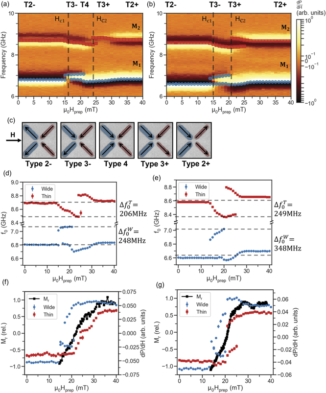
Figure 4. MS orientation remanence FMR and microstate evolution. (a) and (b) Heatmap of differential FMR amplitude vs frequency at a range of preparation fields Hprep in the MS orientation for WM-S (a) and WM-HDS (b) samples. Magnetisation schematics of the type 2−/type 3−/type 4/type 3+/type 2+ microstate trajectory are shown in (c). (d) and (e) Extracted resonant frequencies f0 for the bar-centre localized modes are shown on scatter plots in blue (wide bar) and red (thin bar) for WM-S (d) and WM-HDS (e). Samples were initially saturated in −200 mT before sweeping Hprep 0–40 mT in 1 mT steps and measuring zero-field FMR spectra between each step. Coercive fields are marked Hc1 (wide) and Hc2 (thin), accompanied by a phase reversal of the relevant mode in the differential plot. (f) and (g) MOKE measured remanence magnetisation (black trace, left y-axis) and FMR amplitude of wide bar (blue trace, right y-axis) and thin bar (red trace, right y-axis) modes for WM-S (f) and WM-HDS (g).
Download figure:
Standard image High-resolution imageAs the population of type 3 and type 4 vertices grows the local dipolar field landscape changes, shifting the resonant frequency of both modes figures 4(c) and (d). Due to quenched disorder, type 3+ vertices populate the sample gradually. Type 3+ vertices increase M1 mode splits as the reversed wide bars blueshift and the M2 mode gradually redshifts. Once Hprep > Hc1 the population of type 4 vertices increases, resulting in greater blueshift in M1 and redshift in M2 until the maximum type 4 population is reached. For the WM-S (WM-HDS) samples total M1 blueshift is 248 ± 4 MHz (348 ± 19 MHZ) while the M2 redshifts 206 ± 15 MHz (249 ± 7 MHz). In the MS orientation the resonance frequency continuously shifts due to gradually changing the average local dipolar field from the ensemble of microstates throughout the reversal process. The mix of vertex population and quenched disorder leads to a more disordered transition into and out of type 4 and consequently creates a more varied dipolar field landscape.
Using Kittel fits, the relative MS orientation shift in dipolar field between type 2 and type 4 states is 8.6 ± 0.2 mT (10.6 ± 0.1 mT) and 10.5 ± 0.1 mT (15.0 ± 0.3 mT) in WM-S (WM-HDS) for thin and wide bars respectively. Point dipole modelling estimates bar centre-point shifts of 7.2 mT (11.6 mT) and 4.5 mT (7.3 mT) for WM-S (WM-HDS) in thin and wide bars respectively. The simulated dipolar field estimate underestimates the dipolar field shift in the wide bars again due to neglecting realistic magnetisation textures such as edge curling influence on the mode shift.
Extracted M1 and M2 amplitudes are shown in figures 4(e) and (f) along Mr for WM-S and WM-HDS samples. The MS orientation remanence magnetisation curve does not show a distinct magnetisation plateau due to the similar coercive fields of the thin and wide bars in this direction. In FMR measurements the distinct resonance frequency of the thin and wide bars allows each subset to be probed individually, in contrast to conventional magnetometry which can only access the bulk magnetisation. The FMR differential amplitude of M1 and M2 correspond well with the remanence magnetisation measurement.
3.4. Remanence FMR of symmetric square ASI
We now apply spectral fingerprinting to the S-S sample, while width-modified samples follow a well-defined microstate trajectory during reversal, the S-S sample evolves through disordered microstates with mode frequencies determined solely by local dipolar field texture and quenched disorder.
Figure 5(a) shows the MOKE hysteresis loop with highlighted remanence magnetisation traces at a range of Hprep and corresponding to the prepared microstates identified via MFM images (figures 5(c)–(e)) and differential FMR spectra (figure 5(b)). The sample was saturated along −x before measuring MFM and FMR. Spectra exhibit two dominant modes corresponding to unreversed  , (−x magnetized, 20 mT trace) and reversed
  (+x magnetized, 30 mT trace) bars, with partially reversed microstates a combination of both (i.e. 24.4 mT trace). Figure 5(f) shows remanence spectral heatmaps with Hprep = 20–30 mT, 0.2 mT steps. We observe 2 additional lower intensity modes in addition to the dominant bulk centre-localized mode M1, corresponding to bulk edge-localized E1 and the edge E2 modes with simulated spatial powermaps for each mode. All modes exhibit characteristic sign change (figure 5(g)) of
  around Hc associated with magnetisation reversal.

Figure 5. Remanence FMR and microstate evolution of S-S ASI. (a) MOKE Hysteresis-loop of S-S sample showing remanence traces at Hprep = 20, 23.2, 24.4, 25.6, 30 mT. (b) Remanence FMR spectra for microstates corresponding to Hprep values from MOKE and MFM measurements. (c)–(e) MFM images of microstates corresponding to the same intermediate Hprep values are shown on MOKE loop and FMR spectra. (f) Remanence FMR heatmap for Hprep = 20–30 mT, 0.2 mT field steps, 20 MHz frequency steps with normalized spectral powermaps of centre-localized bulk mode M1, edge-localized bulk mode E1 and edge mode E2. (g) Fitted resonance frequency of M1 mode (black) as a function of preparation field Hprep with point dipole modelled resonance frequency shift of the positive  (blue) and negative
  (red) modes, where the transparency corresponds to the amplitude of the mode. (h) Remanent MOKE magnetisation (black, left y-axis) and FMR power (blue, right y-axis) as a function of Hprep.
Download figure:
Standard image High-resolution imageAt remanence, isolated reversed and unreversed bars will have the same resonant frequency. However, in a lattice the surrounding bars and lattice imperfections lead to resonant frequency shifts throughout reversal. Within the coercive field distribution both  and
and  contribute and are identified via careful fitting of two opposite sign differential Lorentzian curves. The extracted f0 figure 5(f) shows a characteristic asymmetric frequency shift around Hc from the combination of local dipolar field texture and quenched disorder.
The distribution of coercive fields over the sample follows a distribution of bar dimensions due to imperfections in the nanofabrication (quenched disorder) which varies the demagnetisation factors and hence f0. This can be interpreted as a distribution of widths with on average wider bars having lower Hc and lower f0. These bars will typically reverse at lower field and upon reversal will be surrounded by unreversed neighbouring bars, experiencing local dipolar field oriented opposite their magnetisation. This reduces Heff and hence redshifts f0. The total frequency shift for reversed bars is a sum of the redshift due to quenched disorder and local dipolar field  . The corollary of these arguments is that bars reversing at higher fields typically have higher shape anisotropy and hence higher f0. The dipolar field frequency shift will still result in an f0 redshift as the symmetry of the argument remains the same and so the total frequency shift for unreversed bars is
  . This asymmetry in the contribution of the dipolar field to frequency shift results in
  showing a smaller frequency shift than
  throughout reversal. In figure 5(g) simulated curves generated via point dipole simulation are superimposed for the reversed (red) and unreversed (blue) bar populations, including quenched disorder of 4% and converting Heff at each bar to f0 via results from MuMax3 simulation. Close correspondence is observed between measured and simulated behaviour, confirming the attribution of the initial low field increase in f0 due to quenched disorder and the later higher field sharp decrease in f0 to the local dipolar field texture. Crucially, this allows absolute measurements of both. Deconvoluting these effects in strongly interacting magnetic nanoarrays is historically extremely challenging, and the demonstration here is a key strength of the spectral fingerprinting method.
Figure 5(h) shows a comparison of MOKE remanence magnetisation measurement (black curve, left y-axis) with M1 FMR amplitude. As in figures 3 and 4(f)–(g), an extremely close correspondence is observed—illustrating the effectiveness of spectral fingerprinting at elucidating not just fine microstate details, but also the system magnetisation.
3.5. Remanence FMR analysis of multiple M = 0 microstates
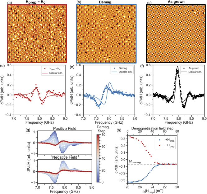
Here we compare three M = 0 microstates; prepared by applying Hprep = Hc after negative saturation (figure 6(a)), AC field demagnetisation (figure 6(b)), and as grown (figure 6(c)). Macroscopic magnetisation measurements are unable to distinguish between these M = 0 states, but their remanence FMR spectra are distinct due to different local dipolar field textures in each microstate. The microstate in figure 6(a) is dominated by small domains of type 2 vertices magnetized in random directions, the microstate in figure 6(b) is a roughly equal mixture of type 1 and randomly oriented type 2 domains and the as grown sample is close to perfectly periodic type 1 order. Figures 6(d)–(f) shows the remanence spectra for the three microstates. Using the MFM images, the local field at the centre of each bar was estimated using dipolar simulations. The resonance frequency was estimated from the local dipolar field and Kittel fits of the S-S sample with the field. Summing together differential Lorentzian peaks for each macrospin gives the dipolar sim. curves shown in figures 6(d)–(f). This allows for the full microstate from the MFM images to be included in the spectral response. The Hc state spectra shows a low amplitude mode indicating a wide distribution of dipolar field landscapes with equal populations of negatively and positively magnetized bars, reflected in the low amplitude of the simulated curve.
Figure 6. Remanence FMR of multiple M = 0 Microstates. (a)–(c) MFM images of the S-S sample taken in three M = 0 states. The as grown state (a), AC-field demagnetized state (b) and a state prepared by applying positive field equal to Hc after negative saturation (c). (d)–(f) Remanence FMR spectra of the three M = 0 states shown in MFM images (a)–(c) as a scatter plot with dipolar simulations using the microstate shown above of the FMR spectra plotted as a line. (g) Remanence FMR spectra in both positive and negative preparation-fields from 28 mT to 20 mT measured during an AC field demagnetisation process with field steps of 0.1 mT. Colour bar indicated field magnitude applied before measuring remanence spectra. (h) FMR mode amplitude measured during AC field demagnetisation. FMR amplitude is presented both as a function of demagnetisation step number (top x-axis) and absolute preparation-field magnitude (bottom x-axis). The residual mode amplitude after demagnetisation due to remaining net magnetisation Mdemag is indicated by the dashed line.
Download figure:
Standard image High-resolution image
The demagnetized state shows a shift in the resonance frequency because of the high population of type 1 states but only a single magnetisation direction. The progression to the demagnetized state can be seen in figures 6(g) and (h) as remanence FMR spectra were measured throughout AC demagnetisation from 28 mT − 20 mT in 0.1 mT steps. The sample starts in a saturated type 2 state and as the preparation field is reduced, bars with higher-than-average coercive field lock into the last magnetisation state where the field was large enough to reverse. As the Hprep spectra in the positive field direction changes phase while in the negative field direction it remains the same and the net FMR power does not reach zero (figure 6(h)). This is evidence of residual magnetisation Mdemag due to the imperfection of demagnetisation routines in reaching the GS [24, 38]. The different populations of type 1 and type 2 vertices results in the difference between the M = 0 spectra.
In the as grown state the vertices of square ASI will tend towards type 1 (figure 6(c)) as the lowest energy configuration. The spectrum (figure 6(f)) shows a superposition of  and
and  with a slight shift in frequency between the two modes, however, the antiferromagnetic ordering of the GS results in an identical dipolar field on both the positively and negatively magnetized bars. In zero-field this will result in a cancellation of the positively and negatively magnetized modes. However, incorporating a slight magnetic field of −0.5 mT, possibly due to trapped flux, into the simulation reproduces the splitting of the
  and
and  modes. Despite the small sample area of the MFM measurements the simulated and experimental spectra for the M = 0 microstates agree very well. The ability to distinguish between equal magnetisation microstates using a fast and low power technique is essential for readout in reservoir computation.
4. Conclusion
We have demonstrated 'spectral fingerprinting' across a range of strongly interacting nanomagnetic arrays. Via zero-field FMR, spectral fingerprinting bridges the gap between bulk magnetisation measurements such as MOKE or VSM, and single macrospin resolution microstate mapping such as MFM or PEEM. Operating at a fraction of the time of single macrospin mapping and inherently scalable (demonstrated here on mm scale arrays), spectral fingerprinting provides information unavailable using net magnetisation measurements. Measuring microstate dependent absolute dipolar field magnitude has long been a goal of research into interacting nanomagnetic systems. Here we have provided an elegant solution requiring an off the shelf FMR system, with the underlying methodology equally applicable across alternative spin-wave measurements such as Brillouin light scattering [39, 40]. While the experiments performed here rely on the global field to prepare microstates, however, local control of the microstate [41, 42] eliminates the dependence on magnetic field. Our demonstration here has concentrated on ASI, spectral fingerprinting is ideally suited across a range of interacting nanomagnetic systems particularly the burgeoning range of 3D artificial spin systems where single macrospin imaging is inherently much harder [28–30]. Additionally, spectral fingerprinting is an attractive state readout solution for recent neuromorphic and wave computation schemes harnessing the vast set of microstate spaces for next-generation computing [4–7], with it already having been demonstrated for reservoir computing [31].
Author attributions
AV, JCG, WB conceived the work. JCG, KDS fabricated the samples. AV performed experimental MOKE measurements and FMR measurements. AV performed analysis of FMR measurements. AV, JCG, KDS performed MFM measurements. AV wrote code for dipolar needle modelling and conversion to FMR spectra. DMA, TD wrote code for simulation of magnon spectra. AV drafted the manuscript, with contributions from all authors in editing and revision stages.
Acknowledgments
This work was supported by the Leverhulme Trust (RPG-2017-257) to WRB. TD and AV were supported by the EPSRC Centre for Doctoral Training in Advanced Characterisation of Materials (EP/L015277/1). Simulations were performed on the Imperial College London Research Computing Service [43]. The authors would like to thank L Cohen of Imperial College London and H Kurebayashi of University College London for enlightening discussion and comments, and D Mack for excellent laboratory management.
Data availability statement
The data that support the findings of this study are available upon reasonable request from the authors.