As good as it gets: a scaling comparison of DNA computing, network biocomputing, and electronic computing approaches to an NP-complete problem

Ayyappasamy Sudalaiyadum Perumal; Zihao Wang; Giulia Ippoliti; Falco C M J M van Delft; Lila Kari; Dan V Nicolau

doi:10.1088/1367-2630/ac3883

1. Introduction

Nondeterministic polynomial time complete (NP-complete) problems are the mathematical representations of many and very diverse real-life applications, such as protein design [1] and folding [2], data clustering in networks [3], circuit verification [4], optimal routing [5], and formal contextual reasoning [6]—to name just a few. Because of the exponential increase of the solution space with the problem input size, electronic computers—including high-end supercomputers—cannot solve large instances of NP-complete problems, since they operate with limited parallelism at best. Electronic computers face additional difficulties, such as reaching their fundamental physical limits of the gate size, which is already in the couple of nanometers, or engineering-related limits, e.g. required energy, and heat dissipation. All these difficulties challenge the sustainability of Moore's law [7, 8], which predicts the doubling of computing power approximately every two years. Consequently, alternative computational paradigms capable of massively parallel operations were proposed since the mid-1990s [9, 10]. Inspired by the natural massive parallelism of biological systems, many of these alternative computational paradigms use biological entities, from molecular to cellular, in vitro or in vivo, to solve computational problems. The large variety of biocomputation approaches combined with the fact that they are not yet standardized, precludes a direct comparison of their respective scalability, as well as a comparison with the 'classical' electronic computing.

This study compared key performance parameters of three fundamentally different computing approaches: two massively parallel biocomputation approaches, that is, the DNA computing [9], DNA-C, and the more recently reported network biocomputing using motile agents [11, 12], NB-C; with the classical electronic computing, (E-C). To achieve a fair analysis all these computing approaches were employed to solve the same benchmark NP-complete problem, that is, the subset sum problem (SSP). Because quantum computing (QC) is presently evolving very fast, with a large variety of reports regarding performance parameters, and with no report of solving SSP, the present scaling comparison could not be extended to QC. In comparing the DNA-C, NB-C, and E-C approaches for solving SSP, the key operating parameters surveyed comprised the pre-computing costs (section 3.1), the volume need for the computation (section 3.2), the run time (section 3.3), and the energy costs (section 3.4), all calculated using the experimental parameters and estimation methodology reported previously [11–13]. Potential solutions, including hybrid computing approaches, are discussed in section 4.

2. Solving the Subset Sum Problem with various computational approaches

2.1. NP-complete problems and the Subset Sum Problem

A problem is called nondeterministic polynomial time (NP) if a guessed solution can be verified in polynomial time, where 'nondeterministic' means that no particular rule is used to make the guess [14]. A characteristic feature of NP problems is that all known algorithms for solving them take a computing time that grows exponentially with the input size. Whether or not polynomial time algorithms exist for NP problems is one of the foremost open problems in computer science. If a problem is NP, and all other NP problems are reducible to it in polynomial time, then the problem is called NP-complete. It follows that, if a polynomial time algorithm were found for a single NP-complete problem, then all NP problems would be solvable in polynomial time (it is widely believed that this is not the case). Thus, every NP-complete problem is significant, and one of the most well-known NP-complete problems is the SSP, defined below.

The subset sum problem (SSP, see e.g. [15]), asks the following yes/no question: 'given a finite input set S ⸦ $\mathcal{N}$ of positive integers and a positive integer target number t ∈ $\mathcal{N}$ , does there exist a subset ${S}^{\prime }$ ⊆ S such that $t={{\Sigma}}_{s\in {{S}^{\prime }}^{S}}$ ?' Note that other variants of SSP allow the input set S to be a multiset, which allows repetitions of its elements. An instance of SSP consists of a particular set S and a particular target number t, and the size of the instance is defined as the cardinality of the input set S. Note that each instance of SSP has a yes/no answer. For example, for the SSP instance of size 3 with input set S = {2, 3, 9} and target number t = 5, the answer is 'yes', and the subset of numbers that add up to t = 5 is ${S}^{\prime }$ = {2, 3} (the 'yes' answer is the solution to this instance of the problem). In computer science, solving SSP means finding an algorithm that outputs the correct solution (yes/no answer) for all instances. In the case of a 'yes' answer, there is the optional step to identify the subsets that fulfill the required condition. Both variants of SSP (the yes/no answer variant, and that of listing all solutions in the case of a 'yes' answer) are NP-complete.

Unconventional biocomputing approaches to solving instances of NP-complete problems used a large variety of biological agents, from DNA molecules to multicellular organisms (table 1 provides a non-exhaustive summary).

Table 1. Unconventional biocomputing approaches to solving instances of NP-complete problems. Only biocomputation procedures that were experimentally demonstrated are included.

Agent	Problem	Cardinality	Methodology	References
DNA	Directed HPP	7 nodes	Annealing, PCR, extraction, gel electrophoresis	[9]
	Maximal independent set	6 vertices	Cutting, pasting, cloning, gel electrophoresis, sequencing	[16]
	Minimal dominating set	6 vertices	Protein expression, cutting, pasting, cloning, PCR, gel electrophoresis	[17]
	Knapsack/SSP	7	Protein expression, cutting, pasting, cloning, gel electrophoresis, sequencing	[13]
		3	Pasting, PCR, gel electrophoresis, annealing, sequencing	[18]
		3	Cutting, pasting, gel electrophoresis, annealing	[19]
	Satisfiability (3-SAT)	6 and 20 variables	PCR, sequencing, extraction, gel electrophoresis, annealing, pasting	[20, 21]
		3	Extraction, exonuclease digestion, PCR, annealing	[22]
		6	Annealing (hairpins), cutting, pasting, PCR, sequencing, gel electrophoresis	[23]
		4	Competitive hybridization, extraction	[24]
		4	Cutting, pasting (ligase chain reaction), gel electrophoresis, cloning, extraction, sequencing	[25]
	Maximal Clique	6 vertices	Annealing, overlap extension by polymerase chain reaction (PCR), gel electrophoresis, cloning, sequencing, cutting	[26]
	Maze	10-vertex rooted tree with three junctions	Strand displacement, hybridization chain reaction	[27]
Motor proteins	SSP	SSP N = 4	Nano-fabricated microfluidic network-based	[11]
Amoebae	Maze	5-by 5-unit cell maze	Macroscopic network network-based	[28]
Bacteria	HPP	3	In vivo cell based	[29]
	Maze	10-by 10-unit cell maze	Nutrient stimuli-based solutions	[30]
	Maze	15-by 15-unit cell maze	No-nutrient stimuli, non-reward system	[31]
Slime mold	Steiner tree	Up to 12-point	Agar based network paths using plastic boundaries	[32, 33]
	HPP (TSP)	20 cities	Agarose based surface spots representing the cities	[34]
	Maze	5-by 5-unit cell maze	Macroscopic network network-based	[28]
Fungi	Maze	15-by 15-unit cell (open mazes)	No-nutrient stimuli, non-reward system	[35]
Fungi	Maze	Small and large mazes	No-nutrient stimuli, non-reward system	[36]
C. elegans	Maze	Six T-maze and complex U-maze	Macroscopic networks	[37]
	TSP	6 station	Large rooms (7 m by 5 m) with selected station as 2D color patterns	[38]
	Maze	5 by 4-unit cell (unique solution)	Compartment based, macroscale	[39]
Ants	Maze	16 by 16	Non-unique maze solutions	[40]
	Maze	14-unit T-maze	Chamber type of units, reward and non-reward maze-solving strategies	[41]
Complex organisms,		8-arm radial maze		[42]
e.g., rats, mice,		8-arm radial maze		[43]
pigeons, etc		8-arm radial maze		[44]
		8 arm and 4-arm radial maze		[45]

2.2. DNA computing (DNA-C)

This section presents an overview of the main idea behind DNA-C, as well as the molecular biology tools used for the implementation of DNA-C, followed by a detailed description of the wet lab implementation of DNA-C procedure for solving several instances of SSP, based on a previous report [13].

2.2.1. DNA computing overview

In the same way the letters of the alphabet are used to write text, and the bits 0 and 1 are used to write computer machine code, the four basic DNA units, adenine (A), cytosine (C), guanine (G), thymine (T), are used by nature to write genetic information as DNA strands. The possibility of encoding symbolic information on DNA, and the fact that biochemical processes such as cut-and-paste of DNA strands have been proved to be able to implement arithmetic and logic operations, led to the development of the field of DNA-C and molecular programming [9]. The three main steps of a DNA-C are: (1) encoding the input information as DNA strands, (2) DNA computation, and (3) reading the output of the DNA computation.

Step 1: encoding information as DNA. A DNA single strand consists of four different types of units called nucleotides or bases strung together by an oriented backbone, the distinct ends of which are denoted by 5', and 3', respectively. Moreover, A can chemically bind to T, while C can similarly bind to G, in a process called Watson–Crick complementarity (or simply complementarity). Two DNA single strands with opposite orientation and with complementary bases at each position can bind to each other to form a DNA double strand in a process called base pairing.

To encode information using DNA, one first selects an encoding scheme, mapping symbols onto strings over the DNA alphabet {A, C, G, T}, and then proceeds to synthesize the obtained information-encoding strings as DNA single or double strands. For example, the letters of the Latin alphabet were encoded using triplets, e.g. a = CGA, b = CCA, c = GTT, d = TTG, e = GGT, r = TCA, n = TCT, o = GGC, and t = TTC, etc [46]. With this encoding, the English text 'to be or not to be' becomes the DNA strand

5'—TTC GGC CCA GGT GGC TCA TCT GGC TTC TTC GGC CCA GGT—3'

which can be readily synthesized. DNA synthesis is the most basic biochemical operation used in DNA computing. DNA solid-state synthesis is based on a method by which the initial nucleotide is bound to a solid support, and successive nucleotides are added step-by-step, from the 3' to the 5' direction, in a reactant solution. While the above encoding example is purely hypothetical, DNA strands of lengths of up to 1000 bp can be readily synthesized, using fully automated DNA synthesizers, in under 24 h [47]. The synthesis of DNA strands longer than 10 kbp is more challenging and time consuming. There are two major approaches to synthesizing such strands, i.e. chemical synthesis and enzymatic synthesis, both involving multiple rounds of synthesis of short DNA fragments, followed by their assembly into longer DNA strands. A commonly used tool like BioBrick assembly [48] could take 30 days to 45 days to synthesize DNA strands longer than 10 kbp. The estimate for the total duration to synthesize DNA strands longer than 5 kbp is based on commercial gene synthesizing services like Integrated DNA Technology [49], Codex [50], Twist Biosciences [51], Eurofins [52] and Genscript [53, 54], using the specifications from their respective websites.

In most experiments, DNA-encoded information is not associated to a memory location but consists of free-floating DNA strands which, due to Watson–Crick complementarity, can interact with each other in programmed, but also undesirable ways. Exceptions are surface-based DNA-C experiments [22, 55], wherein data-encoding DNA strands are fixed to a solid surface, raising different challenges.

Step 2: DNA computation. A DNA computation consists of a succession of biochemical operations. The following is a list of the main biochemical operations used in the DNA-C experiments.

(a)
Watson–Crick base pairing (hybridization, annealing), due to the Watson–Crick complementarity of bases (A with T, and C with G), is the principal biochemical operation underlying most, if not all, DNA computations. Watson–Crick base pairing was utilized in the first proof-of-concept DNA-C experiment, which solved a seven-node instance of the Hamiltonian path problem [9]. It was also used in the DNA-C experiment that solved a 20-variable instance of the 3-SAT (satisfiability) problem, which marked the first instance of a DNA computation solving a problem beyond the normal range of unaided human computation [21]. Lastly, Watson–Crick base pairing was the crucial computational biochemical operation used in algorithmic self-assembly of DNA tiles utilized, e.g. for the implementation of logic gates [56], stochastic computing [57], the implementation of cellular automata [58], or in molecular algorithms using reprogrammable DNA self-assembly [59].
(b)
Cutting (restriction enzyme digestion) is a biochemical operation implemented by restriction endonuclease enzymes. Such a restriction enzyme cuts double-stranded DNA into fragments at, or near, an enzyme-specific pattern known as restriction site. The result of cutting a DNA double strand at a restriction site (by cutting the backbones of each of its two component single strands) is either two partially double-stranded DNA strands with single-stranded 'sticky-ends', or two fully double-stranded DNA strands with 'blunt ends'. Some enzymes cut non-specifically, outside their restriction site, and they have also been employed for computations, e.g. in the wet lab implementation of a programmable finite automaton using the FoKI enzyme [60, 61]. The DNA-C experiment that solves an instance of the SSP, described in section 2.2.2, uses two restriction enzymes that each cuts a DNA double strand at a specific recognition site, with the result being two partially double-stranded DNA molecules with sticky ends.
(c)
Pasting (ligation) is a biochemical operation that accomplishes the opposite of cutting. It is implemented by DNA ligase enzymes that can join together DNA strand backbones. Some DNA ligases join together partially double-stranded DNA strands with complementary sticky-ends, while others join together blunt-ended DNA strands.
(d)
Polymerase chain reaction (PCR) is often used in DNA-C experiments to amplify, i.e. produce an exponential increase of DNA single strands called templates. PCR is executed by the DNA polymerase enzyme, which extends a primer (short DNA sequence that base pairs to one end of the template), nucleotide by nucleotide, until it produces a full Watson–Crick complement of the template. This biochemical operation has also been specifically used in the implementation of a finite state machine by hairpin formation, using whiplash PCR [23].
(e)
Gel electrophoresis for separation of DNA strands by length was used, e.g. for extracting the DNA strands encoding the solution to the Hamiltonian path problem [9], or for extracting the solution to the SSP [13].
(f)
Extraction of DNA strands that contain a certain pattern as a substrand, by affinity purification, is a biochemical operation that was used, e.g. [9], for selecting the paths that pass through a given node.
(g)
DNA strand displacement (toehold-mediated or polymerase-based) is a more recent biochemical operation used, e.g. to implement DNA-based artificial neural networks that can recognize 100 bit hand-written digits [62–64]. It was also used in computing the square-root of a number [65], for building full adders and logic gates [66], and to implement chemical reaction networks [67]. In addition, DNA strand displacement was used in localized DNA computing, whereby logic circuits are implemented by spatially arranging reactive DNA hairpins on a DNA origami surface [55], potentially reducing the computation time by orders of magnitude.

Step 3: reading the output of the DNA computation. At the end of a DNA computation, the DNA strands representing the output of the computation can be sequenced (read out) and decoded.

One sequencing method uses special chemically modified nucleotides (dideoxynucleoside triphosphates—ddNTPs), that act as 'chain terminators' during PCR, as follows. A sequencing primer is annealed to the DNA template to be read. A DNA polymerase then extends the primer. The extension reaction is split into four tubes, each containing a different chain terminator nucleotide, mixed with standard nucleotides. For example, tube C would contain chemically modified C (ddCTP), as well as the standard nucleotides (dATP, dGTP, dCTP, and dTTP). In this tube, extension of the primer by the polymerase enzyme produces all prefixes ending in G of the complement of the original strand. A separation of these strands by length, using gel electrophoresis, allows the determination of the position of all Gs (complements of Cs). Combining the results obtained in this way for all four nucleotides allows the reconstruction of the original sequence.

Thousands of genomes have been sequenced since the completion of the human genome project [68], using a technique called shotgun sequencing, whereby short genome fragments called 'reads' are sequenced, and computer programs then use the overlapping ends of different reads to assemble them into a continuous sequence. Such conventional methods for reading the output of a DNA computation, including illumina-based sequencing methods, are straightforward, rapid, and accurate (1% maximum error), and DNA sequences of the size of the human genome (over 3 billion base pairs) can now be sequenced in 1 to 3 days [69]. In contrast with these approaches, nanopore-based sequencing techniques are now preferred for their speed, small size of the sequencer, and convenience of use, despite being more error-prone (10% maximum error). Such single-molecule sequencers could process as many as 16 000 reads simultaneously, by using a parallel operating array of nanopores. Using nanopore sequencing methods, DNA strands of a total length of up to 90 million base pairs (with contiguous DNA strands as long as 60 000 bp being read) can be sequenced in 18 h [69, 70].

The three steps of a DNA-C procedure, described above (encoding the input information as DNA strands, the actual DNA computation, and reading out the output of the DNA computation), were used to solve instances of NP-complete problems, such as the Hamiltonian path problem [9], satisfiability problem [20–22, 71, 72], Knapsack problem and its variant, SSP [13, 18, 19], and maximum Clique problem [26].

2.2.2. DNA computing procedure for solving SSP

Existing DNA-C for solving SSP can be categorized as either theoretical DNA algorithms with no experimental implementation [73, 74], or DNA algorithms with a wet lab experimental implementation [13, 18]. The latter are based on the idea of expressing each subset ${S}^{\prime }$ of the input set S as a unique path in a special type of directed weighted graph, as illustrated in figure 1.

**Figure 1.** An SSP instance of size n with input set S = {s_i│1 ⩽ i ⩽ n} can be represented by a directed weighted graph with (n + 1) nodes and designated start and end vertices, as illustrated above. In this graph, each subset of S corresponds to a unique path from the start node (red) to the end node (green), and vice versa. Any such path has to pass through all the nodes of the graph. If, when connecting node (j − 1) with node j, 1 ⩽ j ⩽ n, the path traverses the top edge (thick line), this indicates that the subset it represents contains the number s_j. If, instead, the path traverses the bottom edge (thin line), this indicates that the subset it represents does not contain the number s_j. The edges are weighted, with the weights of the top and bottom edges being (b_i + c ⋅ s_i), and respectively b_i, for 1 ⩽ i ⩽ n.
Download figure:
Standard image High-resolution image

If the input set is S = {s₁, ..., s_n}, the corresponding graph has n + 1 nodes, a designated start node labelled 0, and a designated end node labeled n. For each 1 ⩽ j ⩽ n, the node labeled j corresponds to the number s_j in S, and two consecutive nodes are connected by exactly two directed edges. Each path between node 0 and node n uniquely represents a subset ${S}^{\prime }$ of S, as follows. The presence or absence of a number s_j in ${S}^{\prime }$ is indicated by the path representing ${S}^{\prime }$ traversing either one, or the other (but not both), of the two edges that connect node (j − 1) to node j: if s_j is in ${S}^{\prime }$ then the path traverses the 'top' edge, and if s_j is not in ${S}^{\prime }$ then the path traverses the 'bottom' edge instead (see figure 1). In addition, the weights of the two edges that connect consecutive nodes are different, so that the length of each start-to-end path (the sum of the weights of its edges) corresponds to the sum of the numbers in the subset that it represents.

This conceptual design can be physically implemented by first encoding each directed weighted edge as a DNA strand of a certain length. This is followed by the generation of a combinatorial library of DNA strands encoding all possible start-to-end paths (concatenations of edges/strands) through the graph, which in turn represent all possible subsets of S. The next step is the physical extraction, from this library, of the DNA strands of the desired length representing the solutions to the SSP instance. The length of such an SSP-solution-representing DNA strand is determined based on the target number t specified by that SSP instance. In practice, experimental considerations dictate the introduction of additional parameters c and b₁, ..., b_n, whereby the weight of the edge signaling the presence of s_i in a subset is (b_i + c ⋅ s_i), while the weight of the edge signaling the absence of s_i in a subset is b_i. For example, the set S itself is represented by the start-to-end path that traverses all the 'top' edges in the graph, and the DNA strand that encodes it has the expected length ∑_1⩽i⩽n (b_i + c ⋅ s_i). In contrast, the empty set ∅ is represented by the start-to-end path that traverses all the 'bottom' edges in the graph, and the (much shorter) DNA strand that encodes it has the expected length ∑_1⩽i⩽n b_i. For a target number t, a subset ${S}^{\prime }$ of S whose elements sum up to t exists, if and only if there exists a start-to-end path in the graph, encoded by a DNA strand of length ∑_1⩽i⩽n b_i + c ⋅ t.

Both [13, 18] are based on the concept above, with [18] solving an instance of SSP of size n = 3 with input set S = {2, 3, 4}, target number t = 5, and parameters c = 10, b₁ = 25, b₂ = b₃ = 20, and [13] solving two instances of SSP of size n = 8 and input set S = {21, 45, 36, 51, 36, 36, 36, 36}, one with target number t = 104 and another with target number t = 174, and parameters c = 1, b_i = 6, 1 ⩽ i ⩽ 8.

The wet lab experimental details of the more recent of the two DNA-C procedures for SSP [13], is described further. For a direct comparison with NB-C, this DNA-C procedure must be applicable also to SSP instances with small numbers in the input set (in particular, numbers smaller than the length of the restriction sites of the enzymes used in the DNA computation). To this end, in the description below, the parameters c = b_i = k, 1 ⩽ i ⩽ n, are used, where k is the length of the restrictions sites of all enzymes employed in the experiment.

The DNA-C procedure for solving SSP comprises three steps: the pre-computing step, the solution generation step, and the result readout step.

In the pre-computing step, the natural numbers comprising the input set S = {s₁, ..., s_n}, of an SSP instance of size n, are encoded into a 'computing region of S' that is inserted into a plasmid (a circular DNA double strand), as follows (figure 2, left panel, top). To each number s_i, 1 ⩽ i ⩽ n, one associates a restriction enzyme e_i with restriction site r_i of length k. In addition, two unique restriction enzymes e_start and e_end, with restrictions sites r_start and r_end (also of length k) are used, as delimiters of the computing region of S, as defined later. The enzymes were chosen so that all restriction sites are different from each other. Each restriction enzyme e_i, i ∈ {1, 2, ..., n} ∪ {start, end}, cuts according to a specific pattern, and its restriction point (the location of its cut) is after the k_i-th base of its restriction sequence, from the 5' end. Also, in this experiment all restrictions sites are palindromic, so k_i uniquely describes the cuts on both strands.

**Figure 2.** The DNA-C procedure [13] for solving an instance of SSP. Left panel, bottom: visual figure legend. Left panel, top: the natural numbers comprising the input set S = {s₁, ..., s_n}, of an SSP instance of size n, are encoded into a 'computing region of S' inserted into a plasmid. Center-left panel: the plasmid is amplified by using some bacteria. Center-right panel: the pool comprising all DNA strands representing candidate SSP solutions is generated, by a succession of split-and-merge substeps, using restriction enzymes, purifications by agarose gel electrophoresis, and ligations. Right panel, bottom: the DNA strands representing the candidate SSP solutions are length-separated by agarose gel electrophoresis. Right panel, top: the DNA sequences of the desired length are extracted, amplified (optionally), and sequenced.
Download figure:
Standard image High-resolution image

Next, for each number s_i, 1 ⩽ i ⩽ n, a DNA strand of length k + (k ⋅ s_i − k) + k = k (s_i + 1), called station is designed, consisting of the concatenation of three sequences: the recognition site r_i, a specially designed 'middle sequence' of length k ⋅ s_i − k, and a second copy of r_i.

In the DNA-C procedure for SSP [13], the enzyme e_start is XbaI and the enzyme e_end is HindIII, with the respective restriction sites shown below, with k_start = k_end = 1:

5'—T^↓CTAGA—3' 5'—A^↓AGCTT—3'

3'—AGATC_↑T—5' 3'—TTCGA_↑A—5'

The input set S will now be encoded by a double-stranded DNA molecule, called the computing region of S, which consists of the concatenation of the recognition site r_start, one station for each of the input numbers s_i, 1 ⩽ i ⩽ n, and the recognition site r_end. The recognition sites and middle sequences were carefully designed so that r_start and r_end occur exactly once (at the beginning, respectively at the end of the computing region of S), and each r_i, 1 ⩽ i ⩽ n, occurs exactly twice in the computing region of S (once at the beginning and once at the end of the station for s_i).

Using this encoding scheme, a DNA strand representing the computing region of the input set S is synthesized and inserted into a base plasmid containing one copy of the recognition site r_start and one copy of the recognition site r_end (with no overlap), by using the respective restriction enzymes and ligation. Care must be taken with the encodings and choice of plasmid, so that the restriction sites occur only in the designated places. As shown in figure 2, center-left panel, this base plasmid is then inserted into bacteria, such as Escherichia coli (E. coli), and amplified (exponentially multiplied) to the amount necessary for the ensuing DNA computation. The generated plasmids are then extracted from bacteria and transferred to a test tube.

In the solution generation step, the objective is to generate the space of all potential solutions for this SSP instance, by creating all different plasmids with a computing region representing a subset of the input set. The computing region of a subset ${S}^{\prime }$ of S will consist of the concatenation of the restrictions site r_start, followed by the ordered concatenation of n DNA strands, each representing the presence or absence of a number s_i in ${S}^{\prime }$ , and followed by the restriction site r_end. More precisely, if the number s_i belongs to ${S}^{\prime }$ then the station of s_i (which includes two copies of r_i) is present at the i-th location in the computing region of ${S}^{\prime }$ , while if s_i does not belong to ${S}^{\prime }$ then a single copy of r_i is present at the ith location in the computing region of ${S}^{\prime }$ . The length of the DNA double strand encoding the computing region of a subset ${S}^{\prime }$ is:

$\begin{equation*}{L}_{\mathrm{D}\mathrm{N}\mathrm{A}}^{{S}^{\prime }}\left(n\right)=k+k\cdot \left(n-\mathrm{c}\mathrm{a}\mathrm{r}\mathrm{d}\left({S}^{\prime }\right)\right)+\sum\limits _{{s}_{j}\in {S}^{\prime }}\enspace k\left({s}_{j}+1\right)+k\left(\mathrm{b}\mathrm{a}\mathrm{s}\mathrm{e}\mathrm{p}\mathrm{a}\mathrm{i}\mathrm{r}\mathrm{s}\right).\end{equation*}$

The generation of the combinatorial library of solution candidates can now proceed by a succession of split-and-merge substeps, as follows (figure 2, center-right panel). The content of the initial test tube T, containing the plasmid with the computing region of S, is evenly split into two tubes T₁ and T₂. Next, while tube T₂ remains intact, the plasmids in tube T₁ are digested by the restriction enzyme e₁ in order to cut out the station representing the number s₁, and the resulting linear DNA molecules are ligated back into circular DNA molecules (after purification by agarose gel electrophoresis, to separate and extract out the DNA strands encoding the station representing s₁). Following this, the contents of the new T₁ and T₂ are merged into a tube ${T}^{\prime }$ , which now comprises plasmids of two types: half of the plasmids have computing region of subsets containing s₁, and the other half of the plasmids have computing regions of subsets that do not contain s₁. This succession of split-and-merge substeps is repeated for each of the remaining numbers in S, resulting in a final tube that contains a combinatorial library of plasmids with computing regions spanning all possible subsets of S.

In the result readout step, the possible solution candidates are separated by high resolution electrophoresis, e.g. non-denaturing polyacrylamide gel electrophoresis, PAGE, or 2% agarose gel electrophoresis. The existence of an SSP solution is determined by the presence or absence of a band on the gel corresponding to the desired DNA strand length (figure 2, right panel, bottom). Optionally, the DNA strands in the band indicating a solution can then be sequenced (figure 2, right panel, top).

More precisely, the plasmids in the final test tube are first cut by the restriction enzymes e_start and e_end, resulting in linear DNA molecules representing all possible subset sum combinations for the set S. If a solution to the given SSP instance exists, that is, if there exists a subset ${S}^{\prime }$ of numbers in S that contains numbers adding up to the target number t (that is, ${\sum }_{{s}_{j}\in {S}^{\prime }}\enspace {s}_{j}=t$ ), then a band with DNA strands of length

$\begin{equation*}{L}_{\mathrm{D}\mathrm{N}\mathrm{A}}^{S}\left(n\right)-{k}_{\mathrm{s}\mathrm{t}\mathrm{a}\mathrm{r}\mathrm{t}}-{k}_{\mathrm{e}\mathrm{n}\mathrm{d}}-\sum\limits _{{s}_{j}\in S{\backslash}{S}^{\prime }}\enspace k{s}_{j}={L}_{\mathrm{D}\mathrm{N}\mathrm{A}}^{S}\left(n\right)-{k}_{\mathrm{s}\mathrm{t}\mathrm{a}\mathrm{r}\mathrm{t}}-{k}_{\mathrm{e}\mathrm{n}\mathrm{d}}-\left[\left(\sum\limits _{{s}_{i}\in S}\enspace k{s}_{i}\right)-kt\right]\end{equation*}$

will be detected on the gel, and the answer to this instance of SSP is 'yes'. In this case one can, optionally, sequence each DNA strand representing an SSP solution, to identify the corresponding subset of numbers in S that sum up to t (there can be several such subsets). To determine such a subset ${S}^{\prime }$ , for every number s_i, 1 ⩽ i ⩽ n, its presence or absence in ${S}^{\prime }$ can be determined by checking the number of occurrences of the recognition site r_i in the DNA sequence representing ${S}^{\prime }$ (two occurrences of r_i if s_i ∈ ${S}^{\prime }$ , and one occurrence of r_i if s_i ∉ ${S}^{\prime }$ ).

Alternatively, if there is no band on the gel corresponding to the aforementioned expected length, then the answer to this instance of SSP is 'no'.

2.3. Network biocomputing (NB-C) for solving SSP

Unlike electronic computers, which perform operations in silico, NB-C uses motile biological agents that explore and perform 'operations' in a physical space, designed according to the problem to be solved. These special features of NB-C have interesting consequences for the scaling of computation.

2.3.1. Technology of NB-C with motile agents

Various implementations of massively parallel computation using motile agents, be they abiotic, e.g. photons [75, 76], beads [77, 78], or biological, e.g. cytoskeletal filaments (actin filaments, or microtubules, propelled by protein molecular motors, i.e. myosin, or kinesin, respectively) [11, 79], microorganisms [31, 36, 80, 81], were proposed to solve NP-complete problems. In most general terms, NB-C with motile agents comprises three stages: (i) design of a graph encoding of the NP-complete problem, which is translated into the layout of a physical network, manufactured by micro- or nano-fabrication; (ii) stochastic exploration of the network by large number of autonomous and independent motile agents, each being analogous to a CPU [12]; and (iii) solution(s) generated as a result of network exploration are derived from the number of agents exiting the encoded network endpoints, and from the agent trajectories. The exploration of the computational networks requires that the motile agents are self-propelled, independent of each other, and easily visible, and to the extent possible reasonably small and moving at reasonable high velocity. Essentially, abiotic motile agents do not fulfill the first desideratum, and consequently NB-C using these agents is fundamentally ineffectual. In contrast, the large variety of motile biological agents offer the opportunity of selecting those that fulfill these requirements. Consequently, the following discussion will refer solely to NB-C. Massively parallel computation employing motile biological agents was proposed to solve NP-complete problems, such as SSP [11, 79]. This computation is a three-stage approach: the first stage is graph-based encoding of a NP-complete problem, which is fabricated to physical network by lithographic techniques. Next, this network is explored stochastically by large number of autonomously motile biological entities independent of each other. Each and every biological agent exploring the network is analogous to a 'moving processor' (pseudo-CPU) [12]. Finally, the solution(s) generated as a result of exploring the networks were derived from the number of agents exiting the networks at the network endpoints and from the agent trajectories.

2.3.2. NB-C method for solving SSP

With the notable exception of the Clique problem [82], all implementations of NB-C with motile agents solved SSP [11, 75, 76], because of the easy, 2D graphical translation into a physical network. Consequently, the following discussion focuses on the details of the implementation of NB-C for solving SSP. NB-C comprises three steps, detailed as follows:

Step 1: pre-computing (encoding NP-complete problem followed by physical fabrication and agent preparation). The encoding of an NP-complete problem into a graph [83], followed by its translation into a physical network, which in addition to the parent graph has set dimensions, e.g. lengths, widths, results into a grid with an array of connected junctions. These junctions (unit cells) impose a set of traffic rules for the exploring motile agents. As long as the agents follow the rules when passing through the junctions, correct solutions will be explored for a problem set [11, 12]. The translation of NP-complete problems, from graphs to vector-based graphical networks, uses computer-aided design tools, e.g. AutoCAD. The designed network has micro- or nano-fluidic dimensions, optimized to allow the seamless exploration by the biological agents obeying junction rules. For example, if protein molecular motor-propelled cytoskeletal filaments are chosen, the network channel dimensions and surface modifications are tailored to accommodate agents to freely traverse the network [11]. The size of a unit cell in the computation network for different biological agents, including sub-cellular motile components to multi-cellular organisms was described elsewhere [12]. While the art of translating NP-complete problems to a physical network remains universal across any agent-based computing, the fabrication approach needs to be optimized for the motile agents used for computation. For example, for bacterial-driven NB-C the fabrication of the silicon masters for computational networks, subsequently replicated by PDMS-based soft lithography, the low resolution SU-8-based optical lithography is sufficient (although e-beam lithography has important advantages). However, for (considerably smaller) cytoskeletal filaments-driven NB-C, high resolution e-beam lithography needs to be used for the fabrication of the computational networks directly in silicon wafers. Furthermore, for bacterial-driven NB-C the PDMS-made computational networks, must be treated with plasma then sealed and filled with nutrient medium conducive for the bacterial-driven network exploration [80], as opposed to the protein motors-functionalized networks used for cytoskeletal filaments, which are uncapped to allow the access to ATP-rich fluids present above the computational space.

The design of the network encoding SSP was firstly reported [83], then demonstrated via its exploration by cytoskeletal filaments [11], photons [75], and recently proposed by bacteria [80, 81]. Although the demonstration of proof of concept in solving SSP by NB-C using motor proteins and cytoskeletal proteins and photons is presently more advanced, microorganisms, especially bacteria, present certain advantages, as follows: (i) resilience in living in confined spaces, without or with limited oxygen (facultative anaerobic); (ii) high speed of up to 0.2 mm sec⁻¹ (for Vibrio comma); (iii) small sizes in the μm-range; (iv) various motility patterns, e.g. closer or away from walls, different and stochastic motility behaviors; (v) availability of a large panoply of molecular techniques for the genetic engineering of bacteria. Additionally, bacteria have the inherent ability to multiply in confined spaces, thereby the possibility to operate, at the theoretical limit, booting the computation with only one agent. If the model bacterium would be the common E. coli, which can be genetically engineered to express fluorescence, and in an active mid-log phase culture, the dimensions of the computing agent would be an average of 0.5 μm by 1 μm. Accordingly, the channel dimensions would be, tentatively, 2 μm width and 5 μm depth. These dimensions would prevent bacteria from making U-turns and other illegal paths, thereby obeying the logic operations in the network junctions.

Step 2: solution generation (stochastic exploration of the network by agents, e.g. bacteria). The design of the SSP computation device using a molecular motor-cytoskeletal protein system follows the benchmark work [11]. The calculation-proper comprises the exploration of the network by motile agents, all starting from the same single-entry point, followed by 'decisions' taken at each junction. The agents operate in junctions similarly to binary operations, i.e. agents traversing across junctions; turning right or left, thus performing computations, that is, adding a zero, or one number to the sum, respectively [11, 12]. The agents enter the network through the entry funnel and continue to traverse the network towards the exits. During the traversal progression, the agents come across three types of junctions: split junctions, pass junctions, and join junctions. Depending on the SSP set, certain networks have also join junctions, where the solution to a particular exit could be reached by more than one route. Split junctions are responsible for splitting the agents across the left or right direction, preferably with equal chances. Agents turning left add +1 to the computation, and agents turning right add zero to the computation. The split junctions are positioned based on the subset-sum sets. In between the split junction corresponding to the subset-sum set, there is an array of pass junctions. The function of the pass junctions is to allow the agents to continue in their original movement without turning. These are the horizontal cross-sections where the motile agent must strictly obey the traffic rule of continuing its trajectory. All split junctions contain join junctions, but not all join junctions are active. The target sums with more than one solution will have a join junction at the corresponding split junction that is active, and these networks are referred to as complexity class II networks [12]. Conversely, the problems that can be solved with unique trajectories belong to complexity class I. Representative SSP networks for complexity class II network route and complexity class I network route are shown elsewhere [12]. During agent-driven computing, a host of other physical factors, like biased turn preferences, interaction with the boundaries of the channels etc, can influence the binary decisions. For instance, when bacteria explore a network, their ability to turn left or right is modulated by chemotactic cues, nutrient foraging, flagellum/a architecture, and interactions with surrounding walls [31, 36, 84]. The speed of exploration of the solution space largely depends on the agent velocity, their ability to multiply in the network, and the booting time. Booting time is defined as the time taken for the minimum number of agents required for computation to enter the network. The three modes of booting operable with agent-based NB-C are detailed elsewhere [12]. It was also proposed [12] that computation could be exponentially enhanced with the bacterial multiplication leading to the computing power that could exponentially build-up in par with the increasing sample sizes. Thus, the use of self-dividing agents, such as bacteria, for NP-complete problems could greatly reduce computing time compared with other non-dividing agents. On the other hand, the small size of the motile agents translates to the necessity for the amplification of their visualization, e.g. by tagging with a fluorescent dye [31, 80, 81].

Step 3: readout of the solutions (generation of the output for bacterial NB-C). To retrieve the solutions of the NP-complete problem, the trajectories of the agents in the network must be recorded using an optical interface, such as a microscope. The various limits of the optical readout interfaces on NB-C were reviewed recently, in particular the various limits of the field of view [12]. A timestamped image recording, necessary to obtain a reliable readout from agent-based computation [31, 80] comprises image acquisition, image post-processing, and agent tracking. The existence of an SSP solution can be verified by checking if there are any agents leaving through the exit representing the target number. In addition, since in the solution generation step a series of images of the whole network was taken, the composition of the subsets that represent SSP solutions can (optionally) be obtained by analyzing the traces of the agents. Image processing tools, e.g. ImageJ Fiji [85, 86] and tracking plugins, e.g. Track Mate (semiautomatics) [85, 87], TrackJ (manual) [87], will process the recorded frames of agent movement in the network. The decoded tracks and the density maps encode the solutions to the respective SSP problem set presented to agent exploration. The readout can be arrived at using three approaches.

(a)
Density maps and backtracking. The sum of all the agent trajectories is projected as heat maps, i.e. spatially-distributed frequencies of agent locations. Depending on the color scheme used, the most taken paths (correct solutions) are brightly colored, or of the highest saturation, while the least taken paths (incorrect solutions) are dark, or of minimum saturation (alternatively, the heat maps can be interrogated for their numerical values). These density maps are used as a qualitative measure, a form of quick parallel readout to arrive at the solutions for a particular set. Although quick, this methodology only delivers the target sums, i.e. the existence of a solution to SSP. The combination of the target sum and the multiple routes for the same exit for complexity class II type SSP can be derived by backtracking and identifying the join junctions.
(b)
Agent counting at the exits of the network. Another methodology is based on counting the number of agents at the exits. This methodology, demonstrated for cytoskeletal filaments-driven NB-C [11], translates into a bar chart with a distribution of agents with the highest relative count for correct exits, versus the lowest relative counts for agents exiting, erroneously, the incorrect exits.
(c)
Continuous tracking of the agents from the entry to the exit. Another methodology would be based on single-particle, continuous tracking, either by manual, semiautomatic, or automatic methods, which can be adapted to track the agent movement in the computation network, thus recording the visited junctions encoding a particular solution.

In addition to these, already demonstrated methodologies, several, more elaborate approaches were proposed, such as switchable tagging of biological agents 'on the fly', which would allow the computational trajectories being stored in the agents as transient or permanent memory [12].

A comprehensive list of experimental procedures and the time taken to solve each stage of the agent-based computation is represented in figure 3. Numerical calculations, such as the total number of agents required to solve SSP of different sizes (cardinality), the network sizes comparison was reproduced, with some modifications, as reported elsewhere [94]. The applied modifications to previous scaling analysis stem from considering different input sets, i.e. unit, prime, Fibonacci, and exponential, as introduced in section 3.

**Figure 3.** The model flow chart of agent-based NB-C and the associated stages. The figure here gives a 'bird's eye view' of the computational operations, such as exploring the network by bacteria; and pre-, and post-computational steps, such as network design and fabrication, bacterial preparation and culture for experimentation, results readout, image analysis, together with the associated required duration.
Download figure:
Standard image High-resolution image

2.4. Electronic computing (E-C)

A review of the electronic computing is beyond the scope of this contribution. However, a balanced comparison of DNA-C and NB-C projected capacity of solving NP-complete problems will benefit from benchmarking it against the equivalent projected performance of electronic computers.

Electronic computers are essentially sequential machines (multi-core computers feature bounded parallelism, at best), and therefore they are inherently challenged by the exponential increase of the number of possible solutions with the size of the NP-complete problem. However, electronic computers do present important advantages in tackling NP-complete problems. First and foremost, the speed of computation is presently running in the billions of operations per second. One of the fastest commercial chips, AMD Threadripper 3990X performs approximately 2.3 million MIPS (million instruction per second), at 4.35 GHz [88]. Second, after more than half a century of technology development following Moore's law [7, 89], electronic computer chips benefit from a deep, large, and fully functional ecosystem, including manufacturing and performance standards, business networks, and last but not least, a large body of elaborate mathematical algorithms and information processing protocols. Third, despite reports of a slow-down in technology development, and of the "end of Moore's law" [90, 91], the semiconductor industry continues to find ways for dramatic improvements.

To ensure a correct comparison between the performance of DNA-C, NB-C, and the benchmark electronic computers with regard to their performance in solving SSP, the latter must perform the calculations by brute force, similarly with the former two massively parallel computation approaches. The basic methodology to solve SSP by various generations of electronic computer chips was described elsewhere [12]. Briefly, a computer program to solve SSP was developed in the C programming language to enable very low-level memory access, efficient mapping to machine instructions, and flexibility. The SSP algorithm was designed to explore all ${\sum }_{0\leqslant k\leqslant n}\left(\begin{matrix}\hfill n\hfill \\ \hfill k\hfill \end{matrix}\right)={2}^{n}$ subsets each of which contains at most n elements, and consequently the running time is of the order O (n ⋅ 2ⁿ). RAM and clock speed being the major factors affecting CPU speed, the computing resources of Intel 286, Intel 386, Intel 486, Intel Pentium Pro were replicated by simulating part of their computer hardware with virtual machines. However, these calculations were dependent on the computing power of the chip, and consequently the fastest chip used could solve SSP instances not larger than n = 50, for the prime input set. Fortunately, the computing time was found to be in a near perfect relationship with the technical parameters of the chips, i.e. MIPS and clock frequency, and this allowed the extrapolation of the computing time for solving SSP at higher cardinalities and for more advanced computer chips (AMD Threadripper 3990X).

3. Scaling comparison of the DNA-C, NB-C, and E-C methods solving SSP

This section comprises a detailed scaling comparison of three qualitatively different methods for solving SSP: the DNA-C of [13] described in section 2.2.2, the NB-C method of [11, 12] described in section 2.3, and the classical E-C implementation of the (sequential) exhaustive search algorithm for SSP, described in section 2.4. As comparison benchmarks, four different types of input sets are considered, drawn from the following sequences of positive integers. The unit sequence is {a_i}_i⩾0, where a_i = 1 for all i ∈ N, the prime sequence {p_i}_i⩾0 consists of all the prime numbers in ascending order; the Fibonacci sequence is {f_i}_i⩾0, where f₀ = f₁ = 1 and f_i+2 = f_i+1 + f_i for all i ∈ N, and the two-exponential sequence is {exp_i}_i⩾0 where exp_i = 2ⁱ for all i ∈ N. The unit set of cardinality n is now defined as comprising the first n elements of the unit sequence, and the prime set, the Fibonacci set, and the two-exponential set (or, simply, exponential set) of cardinality n are similarly defined. For example, for cardinality n = 7, the unit set is {1, 1, 1, 1, 1, 1, 1}, the prime set is {2, 3, 5, 7, 11, 13, 17}, the Fibonacci set is {1, 1, 2, 3, 5, 8, 13}, and the two-exponential set is {1, 2, 4, 8, 16, 32, 64}. Using these sets as inputs for instances of SSP, the DNA-C and NB-C methods for solving the SSP problem are now compared, at different cardinalities, as follows. Section 3.1 discusses the pre-computing step for both methods: the synthesis and length of DNA strands utilized in the case of DNA-C method, and the network fabrication details in the case of the NB-C method. Section 3.2 compares the physical volume of the computation for each method, while section 3.3 compares the energy used by each method in the computation step, and section 3.4 compares the energy needed for computation, for all computational approaches considered.

3.1. Pre-computing

Before considering the 'core' operational parameters of the three computational procedures considered here, it must be observed that—following decades of development and standardization—the classical electronic computers consist of 'ready-made hardware', that is, no substantial pre-computing procedures need to be performed. Furthermore, in most instances electronic computers utilize pre-loaded algorithms, possibly including those solving special cases of NP-complete problems.

In contrast, non-classical computing methods such as DNA-C and NB-C are characterized, due to their considerably less progressed development stage, by a lack of standardization, and they usually offer ad-hoc, problem-dependent, solutions (possibly involving the fabrication of new 'hardware' for each problem). Consequently, while this situation is expected to improve with further development of non-classical computing, a thorough scaling comparison and analysis cannot ignore the necessary pre-computing step for the DNA-C and NB-C methods.

In the case of DNA-C, the pre-computing step (described in section 2.2) comprises the synthesis of the DNA strands representing the computing region of the input set S, followed by their insertion into plasmids, and by the amplification of the plasmids containing the computing region of S. As detailed in section 2.2, for an SSP instance of size n, with input set S = {s₁, s₂, ..., s_n}, the length of the DNA strand representing the computing region of S is ${L}_{\mathrm{D}\mathrm{N}\mathrm{A}}^{S}(n)$ . Figure 4 illustrates the lengths of computing regions of the unit, prime, Fibonacci, and two-exponential input sets of various cardinalities, if the length of all restriction enzyme recognition sites is k = 6, see [13]. Using these calculations, and taking 10 kbp as the maximum length of synthesizable DNA strands (see section 2.2), it follows that the largest input sets that can be encoded using this DNA-C procedure and current technology are input sets of cardinality n = 1665 for unit sets, n = 30 for prime sets, n = 15 for Fibonacci sets, and n = 9 for exponential sets.

**Figure 4.** Logarithmic scale graph illustrating the length of the DNA strand that encodes the computing region of the input set in the DNA-C procedure [13], for the unit, prime, Fibonacci, and two-exponential input sets of different cardinalities, from n = 1 to n = 100. The length of the computing region of the input set grows exponentially (linear growth, at logarithmic scale) for two-exponential and Fibonacci input sets, and it grows linearly for unit and prime input sets (quasi-constant growth, at logarithmic scale).
Download figure:
Standard image High-resolution image

The possible rate limiting factors for DNA-C include: (i) despite the high-fidelity DNA-polymerase based amplification, random errors still occur [92, 93]; (ii) DNA fragment hybridization mismatches [94, 95]; (iii) metastable DNA hybrid structures, e.g. hairpin loops [96–98]. However, these errors can be mitigated with optimized protocols, e.g. variation of temperature, use of specific enzymes relaxing the hairpin loops and metastable structures [99]. Additionally, the use of new generation sequencing can help the quantification of errors and provide feedback loop for protocol optimization. Consequently, considering these achievable optimization paths, the scaling estimations regarding DNA-C procedure considered only the optimal properties of the DNA strands.

Besides the length of the computing region of the input set, which determines an upper limit on the size of SSP instance solvable by this DNA-C, another limitation on the pre-computing step is the number of restriction enzymes available. This is because encoding of an input set of cardinality n requires (n + 2) restriction enzymes (one for each number in the input set, and one for each end of the computing region of S). Each enzyme must have a distinct recognition site, and all restriction sites must be of the same length k. If k = 6, see [13], the number of known enzymes with different recognition sites of this length is 47, see [100], and this becomes an additional upper limit for the maximum size of SSP instance solvable by this DNA-C procedure.

In the case of the NB-C method, the scaling analysis used the bacteria-operated version, because it offers more opportunities for insight, especially due to the possibility of agent multiplication. In general, NB-C also needs two separate pre-computing modules: (i) micro-, or nano-fabrication of the computational network, using photo- or electron-beam lithography, followed by semiconductor manufacturing proper for the computational device for cytoskeletal filaments-driven NB-C; or for the master mold for microorganisms-driven NB-C, followed in the latter case by PDMS-based soft lithography [11, 101]; and (ii) genetic engineering of the bacterial strain with fluorescence expressing plasmids [31, 80]. The split and pass junctions have an average diagonal length of 106.3 μm for a bacterium agent of an average size of 0.5 μm × 1.0 μm. The diagonal length may vary depending on the bacterial or the motile agents used for computation. The fabrication time for the network is computed based on the total number of junctions in each input sets. A nanometer precise fabrication is necessary for finer cytoskeletal filaments [11, 79], but for e-beam lithography, a higher resolution, coupled with larger channel dimensions, results in a longer fabrication time/unit cell. Another limiting factor is the largest wafer size available to accommodate the computational network, with the most used wafer diameter being 8 inch (12-inch wafer is presently the maximum size). Figure 5 presents the number of unit cells required for a specific cardinality, with the fabrication time being proportional to this number. As for NB-C analysis, the pre-computation processes, e.g. network fabrication, mass production of bacteria, are not included in the assessment of the computing time needed to solve SSP for various cardinalities. The preparation of bacteria for NB-C proceeds once per computation, with a duration allowing several of these preliminary procedures within 12 h. Because the NB-C network encodes a brute force mathematical algorithm for solving SSP, once the key parameters of the geometry are acquired, e.g. number, type, position of the nodes, length and widths of the channels, templates for post-processing rectifiers, and 'ghost lanes' [81], the actual design of the planar layout of the biological agents-driven computer can progress entirely automatically, e.g. using lithography design software.

**Figure 5.** Logarithmic scale graph illustrating the total number of junctions used in the network for the NB-C [12], for the unit, prime, Fibonacci, and two-exponential input sets of different cardinalities, from n = 1 to n = 50. The total number of junctions grows exponentially for two-exponential and Fibonacci input sets, and it grows linearly for unit and prime input sets.
Download figure:
Standard image High-resolution image

To further clarify the design procedure, in the SSP network used, a set of a problem with total sum size ς is encoded in a modular system, i.e. a lattice built from two isomorphic unit cells. One unit cell type contains a pass junction, where agent traffic lines cross without interaction, the other unit cell type has additional split junctions, allowing a change of traffic direction [11, 12, 81]. The elements s_i of the set are represented by one split-junctions-containing unit cell followed by (s_i − 1) pass junction-only unit cells. All elements s_i of the set represented this way are sequentially ordered to obtain a row of ς unit cells. This row forms the basis of the network, which is copied (ς − 1) times and stacked in the direction perpendicular to the row. The concept of this design is presented elsewhere [81]. It should be noted that adding an element in the set results in diagonal upward traffic, whereas skipping an element results in horizontal traffic. Consequently, only a triangular part of the rectangular lattice, starting in the bottom-left corner, is needed. This translation of a set into a triangular network can be fully automated; the time needed scales with ς². Finally, it should be noted that in case the split lanes in the split junctions unit cell can be optionally blocked, one type of unit cell can be employed in the whole lattice, allowing all sets of total size ς to be calculated by the same network [11, 12]. This would considerably reduce the design and fabrication costs for this type of calculation networks.

To summarize, the limitations on the pre-computing step of this DNA-C are the length of synthesizable DNA strands and the number of available restriction enzymes, while the limitations on the pre-computing step of the NB-C method are the fabrication resolution and the size of the silicon wafer to be fabricated. Thus, the precomputing step limits the size of an SSP instance that can be solved by this DNA-C procedure to at most n = 45 for unit sets, n = 30 for prime sets, n = 15 for Fibonacci sets, and n = 9 for exponential sets. Similarly, for the NB-C method used in this comparison, which uses bacteria as the agents and if e-beam fabrication is used, the pre-computing step limits the size of an SSP instance that can be solved by the NB-C method to at most n = 2000 for unit sets, n = 37 for prime sets, n = 16 for Fibonacci sets, and n = 10 for exponential sets.

While serious challenges remain, none relates to a current technological limitation. Even with the present, state-of-the-art technologies, there are several ways to improve performance to scale up the computation, at a cost, as detailed in section 4. However, a fair comparison of the E-C computing time with that of alternative computing approaches, would omit the time cost for pre-computing and readout procedures. For this scaling analysis, only the information from experimentally demonstrated procedures for solving SSP, as reported for DNA-C [13] and for NB-C [11, 12] was used, as well as the performance specifications of typical electronic computers for E-C.

3.2. Comparison of the volume required by computation

In this section, the physical volume required by the DNA-C, NB-C and E-C methods is compared for the computation of a solution to an SSP instance: the volume of the solution comprising DNA molecules for DNA-C, the volumes of the network channels and the biological agents (bacteria) needed for NB-C method, and the volume of the computer for E-C.

For the DNA-C method, the volume of the computation is proportional to the maximum number of DNA molecules, which is reached during the pre-computing step and remains constant afterwards. Indeed, this DNA-C procedure generates all 2ⁿ potential solutions to an SSP instance of input size n, by selectively removing number representing 'stations' from the computing region of the input set. For this volume calculation, it was assumed that each SSP-solution-encoding DNA molecule is present in the same number of copies, and that w_min denotes the weight of the smallest amount of DNA detectable on a gel (with current technology, w_min is 1 nanogram [102, 103]). With these assumptions, the maximum number of molecules that are required during a DNA-C computation can now be computed, based on the maximum number of the shortest SSP-solution-encoding DNA molecules that have a total weight of w_min.

To calculate the number of base pairs of a partially double-stranded DNA molecule with sticky-ends, each base in a sticky-end was assumed to count as 1/2 base pair. With this assumption, the length of the shortest computing region of a subset (the empty set) at the result readout step is ${L}_{\mathrm{D}\mathrm{N}\mathrm{A}}^{\varnothing }\left(n\right)-k\enspace (\mathrm{b}\mathrm{p})$ . To calculate how many of these shortest molecules fit into w_min, the weight of linear double-stranded DNA molecules of length x (bp) is

$\begin{equation*}{W}_{\mathrm{d}\mathrm{s}}\left(x\right)=617.96\left(x-2\right)+2\cdot \left(617.96+18.02\right)=\left(617.96x+36.04\right)\enspace \mathrm{g}\enspace {\mathrm{m}\mathrm{o}\mathrm{l}}^{-1},\end{equation*}$

where the average molecular weight of one internal base pair is 617.96 g mol⁻¹, and the average molecular weight of the two bases at an extremity is (617.96 + 18.02) g mol⁻¹ (this includes the weight of the additional −OH and −H groups at the ends), see [104]. If the DNA double strands are circular, then their weight is W_c(x) = 617.96x g mol⁻¹.

Given that the number of all potential solutions to a given SSP instance of size n is 2ⁿ, it follows that the maximum number ${N}_{\mathrm{D}\mathrm{N}\mathrm{A}}^{\mathrm{max}}\left(n\right)$ of linear DNA molecules encoding the computing region of the input set is:

$\begin{equation*}{N}_{\mathrm{D}\mathrm{N}\mathrm{A}}^{\mathrm{max}}\left(n\right)={2}^{n}\times {w}_{\mathrm{min}}\times {\left[{W}_{\mathrm{d}\mathrm{s}}\left({L}_{\mathrm{D}\mathrm{N}\mathrm{A}}^{\varnothing }\left(n\right)-k\right)\right]}^{-1}\enspace (\mathrm{m}\mathrm{o}\mathrm{l}).\end{equation*}$

It follows that the maximum volume required during this DNA-C procedure equals the total number ${N}_{\mathrm{D}\mathrm{N}\mathrm{A}}^{\mathrm{max}}\left(n\right)$ of plasmids including computing regions of the input set S, multiplied by the weight of one such 'fully-stuffed' plasmid, and divided by the density of DNA in solution:

$\begin{equation*}{V}_{\mathrm{D}\mathrm{N}\mathrm{A}}^{\mathrm{max}}\left(n\right)={N}_{\mathrm{D}\mathrm{N}\mathrm{A}}^{\mathrm{max}}\left(n\right)\times {W}_{c}(b+{L}_{\mathrm{D}\mathrm{N}\mathrm{A}}^{S}(n))\times {d}^{-1}\enspace (\mathrm{m}\mathrm{l}),\end{equation*}$

where d is the density of the DNA solution in g ml⁻¹, and b is the number of base pairs in the part of the base plasmid that is used. Taking b = 2 174 bp, k = 6 bp, w_min = 10⁻⁹ g, and d = 10⁻³ g ml⁻¹ [103], the estimated volumes of DNA molecules in the DNA-C for SSP with unit, prime, Fibonacci and exponential input sets of different sizes are shown in figure 6. If 5l is taken as the maximum size of container that can be handled in a lab setting, the maximum size of an SSP instance that is solvable with this DNA-C procedure is n = 28 for unit sets, n = 26 for prime sets, n = 21 for Fibonacci sets, and n = 17 for exponential sets.

**Figure 6.** The estimated volumes of biological agents (solution of DNA molecules, respectively bacteria) used by the DNA-C and NB-C procedures, and network channel volumes used by NB-C to solve an instance of SSP with unit, prime, Fibonacci, and two-exponential input sets of different cardinalities, from n = 1 to n = 50 (logarithmic scale). Note that the agent volume in NB-C is equal for all various SSP instances of the same cardinality.
Download figure:
Standard image High-resolution image

For NB-C, in the bacterial-driven version, the volume of the computational agents required for solving a particular cardinality of SSP is dependent on the minimum number of bacteria needed for solving a specific cardinality. The minimum number of agents (bacteria) required to solve an SSP instance of cardinality n can be calculated using the Euler coupon collector relation [105], with the Euler–Mascheroni constant $\gamma$ ≈ 0.577 21, as:

$\begin{equation*}{M}_{\mathrm{N}\mathrm{B}-\mathrm{C}}\left(n\right)=2\cdot \left({2}^{n}\cdot \mathrm{ln}\left({2}^{n}\right)+\gamma \cdot {2}^{n}+\frac{1}{2}\right).\end{equation*}$

A more conservative estimation will use a multiplier of the number provided by Euler's relationship for the minimum number of agents to explore the SSP network for a given cardinality. Furthermore, the higher the error rates in junctions, the larger the number of agents needed to solve SSP. According to experimental reports of the bacterial errors, i.e. 0.5% at the pass junctions of SSP networks, a doubling of the value provided by the Euler relationship appears as conservatively justified [12, 105, 106]. The graph in figure 6 presents the minimum volume of the required bacteria. A similar calculation can be made for cytoskeletal filaments, with leading to smaller volume of the computational agents. At the other end of the spectrum, similar calculations can be performed for larger motile species, e.g. from the Euglena genus, leading to considerably larger volume of agents. The volume of agents required during the NB-C approach is ${V}_{\mathrm{N}\mathrm{B}-\mathrm{C}}\left(n\right)={M}_{\mathrm{N}\mathrm{B}-\mathrm{C}}(n)\times {d}^{-1}$ (ml); where d is the density of the agents in solution. Assuming E. coli as the computational agent, with a density of 2 × 10⁹ cells/ml of culture solution [107], the estimated minimum volume of agents required by the NB-C approach is presented in figure 6. This value is equal for solving SSP instances with unit, prime, Fibonacci, and exponential input sets of the same cardinality.

For NB-C however, apart from the total (bacterial) agent volume needed, there is the need to also consider the volume of the network channels. This volume is calculated, using the track lengths in all junction unit cells of a network design, multiplied by the track width and height (for E. coli networks being 2 μm and 4 μm respectively). For the compact complexity class II networks, with unit, prime, and Fibonacci input sets, the network channel volume is moderately expanding with cardinality (figure 6), as many channels (and exits) will be visited multiple times. However, for the (unary coded) two-exponential network, (complexity class I, in which sets can only be reached by one route), the network volume will rapidly increase with cardinality.

For electronic computers, it can be arguably assumed that at the limit, the computing agents are the electrons. Aside of their very small size, given their sequential processing of electronic computers, there is a very small need for 'agents', thus making the discussion regarding the volume of agents superfluous. At the limit, the necessary volume for E-C can be the volume of a computer chip, which is by any account many orders of magnitude smaller than the volumes required for either DNA-C, or for NB-C.

To summarize, the physical volumes required by the DNA-C method, and the (bacterial) agent and network volumes required by the NB-C for solving an SSP instance grow exponentially with the size of the input set. In addition, the volume required by this DNA-C procedure also grows proportionally to the sum of the numbers in the input set. Compared with the NB-C method, the DNA-C method requires orders of magnitudes larger volumes even for unit input sets. For example, the NB-C method to solve an SSP instance with an input set of cardinality of n = 30 requires approximately 1.07 ml of bacteria, while for the same cardinality the DNA-C method requires 14.7 l for unit sets, 68.8 l for the prime set, 7.54 × 10⁴ l for the Fibonacci set, and 7.44 × 10⁷ l for the exponential set.

3.3. Comparison of the computing time

Perhaps the most important performance criterion for comparing various computing methods for solving NP-complete problems is the computing time required to solve a benchmark problem. Indeed, one of the goals of the research into alternative computing methods was to exploit their massively parallelism to shorten the computing time they require to solve NP-complete problems.

The computing time of DNA-C and NB-C procedures comprises three parts: the time required for pre-computing, the time required by the actual computation step (generation of potential solutions), and the time needed to read out the results. The comparison of the computing time in this section refers only to the time required during the actual computation step, called thereafter run time, and excludes the time spent in the pre-computing step (creation the plasmids in the case of DNA-C, and fabrication the network and culturing the bacteria in the case of NB-C). Similarly, the time spent for read-out analysis was not included either, because (i) the process is simple if only the existence of an SSP solution is considered, and (ii) the process of finding the actual solutions could in principle be parallelized and thus achievable with present technologies and depending on cost considerations only.

For the solution generation step of the DNA-C approach, mentioned in section 2.2.2, the DNA-C procedure for solving an SSP instance of size n comprises n split-and-merge steps. Each such step starts by the digestion of half of the plasmid population by restriction enzymes, to cut out a specific number-encoding 'station'. This is followed by purification by agarose gel electrophoresis, to separate and remove the number-encoding 'station' short DNA strands. This is followed, in turn, by the re-ligation of the longer linear strands, which include the computing region of some subset of the input set, back into circular plasmids. Thus, if t_e is the time required for one restriction digestion, t_p the time required for one plasmid purification, and t_l the time required for one ligation, then the estimated run time for this DNA-C procedure solving a size n instance of SSP is:

$\begin{equation*}{T}_{\mathrm{D}\mathrm{N}\mathrm{A}}^{\mathrm{max}}\left(n\right)=\left({t}_{\mathrm{e}}+{t}_{\mathrm{p}}+{t}_{\mathrm{l}}\right)\times n\enspace (\mathrm{s}\mathrm{e}\mathrm{c}).\end{equation*}$

Taking t_e = 0.5 h (1800 s), t_p = 1.5 h (5400 s), t_l = 0.25 h (900 s), see [103], this results in a run time complexity of ${T}_{\mathrm{D}\mathrm{N}\mathrm{A}}^{\mathrm{max}}\left(n\right)=(8100\times n)$ seconds, as illustrated in figure 7, for various values of n.

**Figure 7.** The estimated run time required by DNA-C, NB-C, and E-C procedures for solving an instance of SSP with inputs set of different cardinalities, from n = 1 to n = 100 (logarithmic scale). The real run time of NB-C will be in between the curves depicting scenario (i) (combinatorial run mode) and scenario (ii) (multiplication run mode). The run time of the DNA-C grows linearly with the cardinality of the input set, while the run time of the NB-C and the E-C grows exponentially.
Download figure:
Standard image High-resolution image

The total NB-C run time for solving SSP, as a function of cardinality of the input set, depends on many parameters, but can be modeled as a mixture of two extreme run modes between which the 'real world' operation takes place:

(a)
In the combinatorial run mode [12], the agents enter the network at the starting point with a fixed booting frequency (determined by the effective agent length in a queue and the average agent speed) and proceed on their routes to the exits. The total run time is the time needed to boot all 2ⁿ agents (times the coupon collector's correction for stochastic multiple identical variable combinations [105]), plus the time needed for a single agent to run from start to exit. For low cardinality problems the single agent run time is important, for high cardinality problems, however, this value is eclipsed by the booting time needed for all agents to enter the network.
(b)
In the optimum multiplication run mode [12], a single agent enters at the starting point, and at every split junction agent multiplication occurs (cell division). In case there is only one route to every legal SSP exit (complexity class I network), the total run time equals the longest one-agent run time from start to exit. This would be the case for the strongly expanding exponential set. More compact networks, however, show multiple routes to the same exits (complexity class II network). As a consequence, there will be a rise in traffic density further down the network; and this may lead to traffic jams. In an 'optimistic' scenario, the agents simply wait until there is enough space available for them to proceed further. The total run time is the run time of one agent plus the time needed to 'de-boot' the agents that need to leave the middle exits of the network, which are more visited than those on the edges, with a fixed 'de-booting' frequency (determined by the effective agent length and average agent speed). Again, at low cardinalities, the single agent run time is important, but for high cardinality problems, this value is eclipsed by the 'de-booting' time needed for the agents to leave the exits in the middle part of the network.

In the 'real world', it is very improbable that cell division will occur at every split junction, which could be also slowing down at higher traffic density. Anyhow, the run time versus cardinality plot for a given network will be in between the curves of the scenarios (a) and (b) described above, as also shown in figure 7.

To summarize, the run time for solving SSP by this DNA-C procedure ${T}_{\mathrm{D}\mathrm{N}\mathrm{A}}^{\mathrm{max}}\left(n\right)$ , is linear with the problem size n, in contrast with the exponential relationships for the run time for both the NB-C and the E-C methods. In addition, the run time required by the NB-C method also grows linearly with the sum of the numbers in the input set. Overall, the linear run time of this DNA-C procedure for SSP is its most competitive feature compared with both NB-C and E-C.

3.4. Comparison of energy required for computation

Another key performance criterion, especially for high performance computing, is the energy consumption for computation. The following analysis does not take into consideration the energy consumption for pre-computing procedures or readout, for all the three computing methods considered.

In the computation step of this DNA-C procedure, two operations are employed: cutting (digestion) by restriction enzymes, and pasting (ligation) by ligase enzymes, as described in section 2.2. The restriction enzyme digestion is inexpensive from the point of view of energy consumption, as no external energy is needed [108]. However, ligation is energy-intensive, as ligases consume one ATP (6.3 kcal mol⁻¹ = 26 359.2 J mol⁻¹ of energy, [109]) per backbone nick-sealing event. Ligating two DNA double strands together entails two such nick-sealing events, one for each single strand. This DNA-C procedure comprises n split-and-merge substeps, and each substep entails re-ligating half of the plasmids (namely those from which one number-representing station was cut out). Hence, the energy consumption of the computation step of the DNA-C for an SSP instance of size n is:

$\begin{equation*}{E}_{\mathrm{D}\mathrm{N}\mathrm{A}}\left(n\right)=n\times \left(\frac{1}{2}{N}_{\mathrm{D}\mathrm{N}\mathrm{A}}^{\mathrm{max}}(n)\right)\times \left(2\times 26\enspace 359.2\right)\enspace (\mathrm{J}\mathrm{o}\mathrm{u}\mathrm{l}\mathrm{e}\mathrm{s}).\end{equation*}$

The energy cost for the computation stage of this DNA-C procedure grows exponentially with the input size n, due to exponential growth of the number of strands ${N}_{\mathrm{D}\mathrm{N}\mathrm{A}}^{\mathrm{max}}\enspace (n)$ , as illustrated in figure 8. While the total energy cost grows exponentially with the input size n, this DNA-C procedure is very energy efficient if considering the average electrical power in Watts (energy divided by the run time, analyzed in section 3.3). Indeed, even though the power also grows exponentially with n, for an input set size as large as n = 50 the energy needed is only about 20 W, similar to the energy consumption of an LED light bulb.

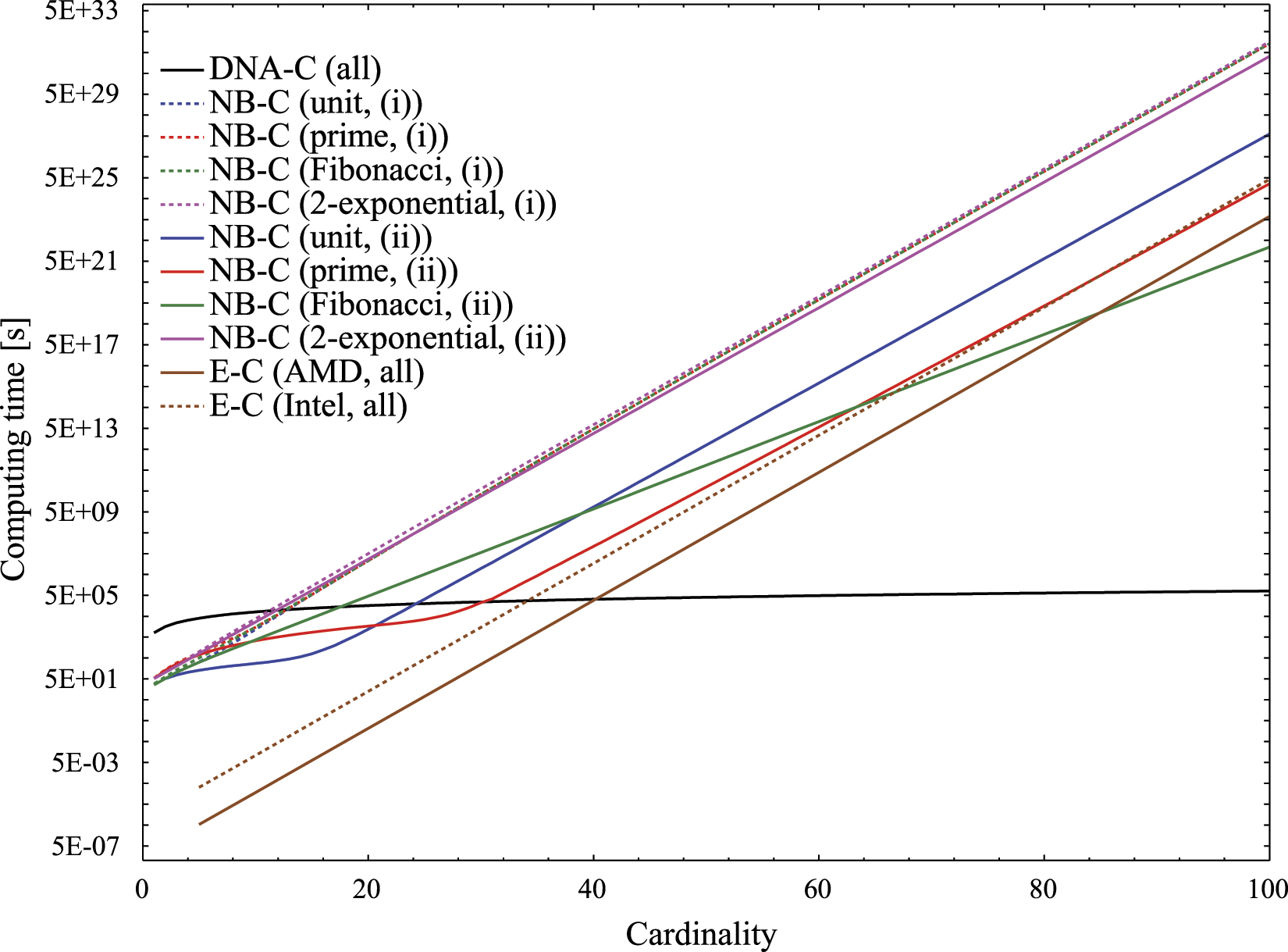
**Figure 8.** The energy required in the computation step of DNA-C, NB-C, and E-C for solving an instance of SSP with unit, prime, Fibonacci, and two-exponential input sets of different cardinalities, from n = 1 to n = 100 (logarithmic scale). The energy cost of the DNA-C and the E-C is independent on the type of input set and depends only on its cardinality, while the energy cost of the NB-C depends on the cardinality, the sum of the numbers of the input set, and the type of agent (here *E. coli* or actin myosin).
Download figure:
Standard image High-resolution image

For the NB-C, the energy required for computation for a given cardinality of SSP, will be determined by the number of agents needed to finish the calculation (including the coupon collector's correction [105]). As the locomotion energy needed for passing one node is known [12], the total energy needed to perform the calculation for the combinatorial run mode (no cell division, scenario (a) in section 3.3), can be easily estimated (figure 8). In the multiplication run mode (with cell division, scenario (b) in section 3.3), on the one hand, the energy required for computation is over-estimated, because many agents originate somewhere in the network and need to run only part of the total track. On the other hand, the energy needed for agent multiplication (cell division) which is likely to cost much more than just running through nodes, was also discounted.

Finally, the energy required by E-C for solving SSP can be easily calculated as the product between the number of operations required by the E-C for solving a particular SSP instance and the energy cost per operation, provided by chip specifications.

To summarize, the energy cost of the computation step for all of DNA-C, NB-C, and E-C grows exponentially with the size of the input set. Moreover, the energy cost in the computation step of the NB-C method also increases linearly with the sum of the numbers in the input set. Overall, the NB-C appears to be more energy-efficient than DNA-C in some cases, i.e. unit, and prime input sets, but in other cases, i.e. Fibonacci and exponential input sets, NB-C is more energy consuming than DNA-C, increasingly so with the increase of the input set cardinality, and regardless of the agents used. However, despite the energy cost being high for NB-C in some cases, bacteria can self-produce the ATP from cheaply available nutrient sources, e.g. beef extract, yeast extract, tryptone, while for DNA-C the ATP must be externally supplied as a purified additive. Therefore, and depending on specific circumstances, bacterial-based NB-C appears to be more self-sustainable [110], despite its sometimes-high energy cost compared to DNA-C. Finally, E-C appears to be an order of magnitude less energy-efficient than both DNA-C and NB-C.

4. Perspectives

The comparison of the DNA-C, NB-C, and E-C computing paradigms, aimed to solve NP-complete problems, each at a very different stages of its development, is based on the current state of the art of enabling technologies. All three approaches present both benefits and drawbacks, when judged against three key performance criteria: volume needed for computation, computing time, and energy needed for computation. A tentative projection of possible future developments, based solely on the present state-of-the-art, is as follows.

(a)
How to address the challenge of a solution space that grows exponentially (or worse) with the size of the problem? All computing approaches analyzed, as well as any other proposed or to be proposed, attempting to solve an NP-complete problem need a computing resource that also grows exponentially with the size of the problem. Therefore, any computing approach attempting to solve an NP-complete problem, must clearly identify, better in the earliest development stages, what is the upper tolerable limit of the critical computational resource that can be plentifully provided, such as DNA molecules, or the area of NB-C network. Alternatively, the computational approach can use an infinite computational resource, such as time, or which can grow exponentially in time, such as self-dividing bacteria, and consequently decide what is the tolerable limit of this infinite of exponentially growing resource. In both cases, these limits on computational resources will translate in the limit of the size of the theoretically solvable NP-complete problem.
(b)
Electronic computing. Despite its advanced age, Moore's law appears to find ways to stay relevant, as witnessed by the continuous, so far, improvement of the performance of individual electronic semiconductor devices, as well as by advances in parallelization of computation. The parallelization can be achieved by multi-core computers, with presently the fastest, i.e. Fugaku, having 7.63 million cores, and the largest, i.e. Sunway TaihuLight, having 10.65 million cores. Moreover, the seriality of E-C results in very small computing volume. This being said, for electronic computers the level of parallelism is bounded by the number of available processors, and this inherently limits the size of the problems that can be solved by a particular computer. Perhaps an even more severe limitation, when compared with alternative computing approaches, is the high energy consumption per operation.
(c)
DNA computing. Although the field originally started with the demonstration of a computing application by Leonard Adleman in 1994, it has shifted its goal away from being a competitor to electronic computers, toward several other promising research and application directions. These include exciting recent developments in ultra-compact DNA-based data storage technologies [46, 111–114], DNA nanotechnology applications [115], shape-programmable 2D and 3D DNA self-assembly, e.g. 3D self-assembly of DNA bricks [116, 117], GDa scale DNA assemblies [118]), DNA origami (e.g. DNA origami polyhedral meshes [119], the world's smallest Mona Lisa image [120], DNA/silica hybrid nanomaterials templated with DNA origami [121]), molecular algorithms using reprogrammable DNA self-assembly [59], DNA nanoscale robots, e.g. DNA nanobots that carry gold particles [122], DNA robots that sort cargo as they walk [123], (see [96] for a review), DNA steganography with SNPs [124], etc.
(d)
Network biocomputing. This more recent and qualitatively different biocomputation approach has advantages, as well as limitations that could potentially be mitigated. First, the encoding of the brute force algorithm in the NB-C network increases the efficiency of the exploration of the solution space. In a sense, NB-C shares the burden of the exponential increase of the solution space with the size of the problem between two, not one, computational resources: the number of computational agents, and the area, and thus the volume of the computer. Second, the functionality of the current NB-C implementation can be improved by tagging the agents 'on the fly' whenever they pass spatially addressable junctions. This would open the possibility of reading the history of logical junctions being visited by agents only at their exit, thus making the optical readout throughout the area of the network obsolete, and therefore making the limitations of the field of view of the optical readout a non-issue. Presently tagging technologies exist, e.g. light-controlled on-off fluorescence, which can be realistically implemented in either cytoskeletal filaments, or microorganisms. Third, NB-C can have 'smarter', albeit possibly larger, agents, which can be genetically programmed to perform slightly more complex functions. If these more complex agents are larger, then the area of the computer will inherently increase, linearly, but if the 'tagging on the fly' technology is developed, and the agents are read only at the exit, the design can progress toward three-dimensional networks, with much more compact footprint, and thus alleviate the need for high resolution lithography, and importantly make the volume of the 'computer' more tolerable. Forth, designs solving other-than-SSP can be developed, e.g. traveling salesman problem, Steiner tree problem, maximal Clique problem, etc. Finally, the 'one-instance/one-network' design issue could be reasonably solved by fabricating templated networks with MEMS-programmable junctions.
(e)
Hybrid computing approaches? The present analysis showed that none of the computing approaches surveyed are superior to all key performance parameters: E-C presents a very small computing volume (due to its seriality), DNA-C has a linear computing time (due to its massive parallelism), and NB-C has a mixture of lower computing volume than DNA-C, but much higher than E-C (due to its encoding of the search algorithm in its networks). While improvements could change the relative ratio of these benefits/drawbacks, it is possible that synergizing these computing paradigms could be the ultimate answer to solving NP-complete problems of reasonable size. Certainly, interfacing such diverse technologies would not be trivial, but there are examples of this synergetic 'technological ecosystem': nuclear plants transform nuclear energy in thermal steam energy, which is then transformed in mechanical energy of turbines, which in turn translates in electrical energy. For instance, aside of calculations, NB-C systems can produce ATP, which can be then funneled to DNA-C (or cytoskeletal-driven NB-C). More importantly, solving NP-complete problems can be 'jump-started' by fast E-C, then the preliminary results can be passed to NB-C, especially with agent division, and finally the large amount of readout data can be stored using the large capacity of DNA memory. That would be as good as it gets.

Acknowledgments

This study was supported by grants from the Defense Advanced Research Projects Agency (DARPA), Grant No. HR0011-16-2-0028, the European Union Horizon2020 FET program Bio4Comp, GA No. 732482, the European Union FP7 program ABACUS, GA No. 613044 to DVN; grants from the Canadian Natural Sciences and Engineering Research Council (NSERC), RGPIN-2016-05019 to DVN, and R2824A01 to LK; and from the Social Sciences and Humanities Research Council of Canada (SSHRC), Grant NFRFE-2019-00129 to DVN and LK.

Data availability statement

All data that support the findings of this study are included within the article (and any supplementary files).

Author contributions

Conceptualization: A Sudalaiyadum Perumal, Z Wang, G Ippoliti, F van Delft, L Kari, D V Nicolau.

Data curation: A Sudalaiyadum Perumal, Z Wang, G Ippoliti, F van Delft, L Kari, D V Nicolau.

Formal analysis: A Sudalaiyadum Perumal, Z Wang, G Ippoliti, F van Delft, L Kari, D V Nicolau.

Funding acquisition: L Kari, D V Nicolau.

Investigation: A Sudalaiyadum Perumal, Z Wang, G Ippoliti, F van Delft, L Kari, D V Nicolau.

Methodology: A Sudalaiyadum Perumal, Z Wang, G Ippoliti, F van Delft, L Kari, D V Nicolau.

Project administration: L Kari, D V Nicolau.

Resources: L Kari, D V Nicolau.

Supervision: L Kari, D V Nicolau.

Validation: A Sudalaiyadum Perumal, Z Wang, G Ippoliti, F van Delft, L Kari, D V Nicolau.

Visualization: A Sudalaiyadum Perumal, Z Wang.

Writing—original draft: A Sudalaiyadum Perumal, Z Wang.

Writing—review & editing: A Sudalaiyadum Perumal, Z Wang, G Ippoliti, F van Delft, L Kari, D V Nicolau.

As good as it gets: a scaling comparison of DNA computing, network biocomputing, and electronic computing approaches to an NP-complete problem

Article metrics

Author e-mails

Author affiliations

Author notes

ORCID iDs

Dates

Abstract

1. Introduction

2. Solving the Subset Sum Problem with various computational approaches