


Abstract
The future forecasting ability of machine learning (ML) makes ML a promising tool for predicting long-time quantum dissipative dynamics of open systems. In this article, we employ nonparametric ML algorithm (kernel ridge regression as a representative of the kernel methods) to study the quantum dissipative dynamics of the widely-used spin-boson (SB) model. Our ML model takes short-time dynamics as an input and is used for fast propagation of the long-time dynamics, greatly reducing the computational effort in comparison with the traditional approaches. Presented results show that the ML model performs well in both symmetric and asymmetric SB models. Our approach is not limited to SB model and can be extended to complex systems.

Original content from this work may be used under the terms of the Creative Commons Attribution 4.0 licence. Any further distribution of this work must maintain attribution to the author(s) and the title of the work, journal citation and DOI.
1. Introduction
With the realization that isolated systems do not exist in the real world, we have to deal with open quantum systems, where we need to consider that the system and the surrounding environment can exchange energy, particles and/or quantum phase. Spin-boson (SB) model is one of the well-known models, which is widely used to understand the effects of the surrounding environment on the system. SB model describes a two-state system coupled to infinite number of non-interacting harmonic oscillators. Understanding quantum dissipative dynamics of SB model (or in general an open quantum system) has applications in wide range of settings such as quantum computing [1], quantum memories [2], quantum electrodynamics [3, 4], organic solar cells [5], superconducting junctions [6], quantum biology [7], quantum optics [8], quantum transport [9, 10], defect tunnelling in solids [11, 12], quantum dots [13, 14], and colour centres and Cooper pair boxes [15, 16]. In addition, SB model has remained a key-model for testing and comparison of open quantum system theories before extending them to complex systems. A large number of numerical methods has been developed to study SB model such as numerical renormalization group method [17, 18], the density matrix renormalization group method [19, 20], the quantum Monte Carlo method [21, 22], the time evolving density matrix using orthogonal polynomial algorithm [23, 24], the reaction coordinate mapping [25], the multi-configuration time-dependent Hartree method [26, 27] and its extensions [28], the Nakajima–Zwanzig generalized quantum master equation [29, 30], transfer tensor method [31–33] and numerical variational method [34]. Regardless of their success, these methods have there own limitations in applicability and accuracy.
In addition to these methods, another popular approach is classical mapping-based approach (Meyer–Miller–Stock–Thoss mapping [35–39], spin-based mapping [40, 41] and so on), where system and surrounding environment dynamics is described by classical trajectories. Classical mapping-based approaches are more feasible, but because of the classical description, in some cases, especially at low temperature, they may fail to correctly describe nuclear quantum effects [39]. Coming back to exact quantum methods, Makri and coauthors proposed quasiadiabatic propagator path integral (QUAPI) scheme [42, 43]. In QUAPI approach, all correlation effects are included over a finite time τ = Kδt and correlation effects beyond τ are neglected. Good convergence requires time τ to be as large as possible and the Trotter increment δt as small as possible. In QUAPI approach, the growing computational cost with the increase of system size and time τ limits its applicability for large complex systems.
An alternative numerical exact benchmarking approach is the hierarchical equations of motion (HEOM) [44–53] approach pioneered by Tanimura and Kubo [54]. HEOM approach captures the combined effects of system–environment dissipation, non-Markovian memory effect, and many-body correlation in a non-perturbative manner. In this approach, a hierarchy of deterministic differential equations are constructed by using a set of memory basis functions to unravel the correlation function of the environment. The size of HEOM depends on two factors; the number of memory basis functions M and the depth of the hierarchy L, both of which depend critically on the strength of the system–environment interaction and many-body correlation. In the case of low temperature and strong dissipative interaction, good convergence requires large M and L, which inevitably makes HEOM approach rather expensive. Such a drawback has restrained the use of HEOM method in the ultra-low temperature regime.
Another approach with no temperature limitation, is the trajectory-based stochastic equation of motion (SEOM) approach. In stochastic formulation, the influence of environment on the system is captured by stochastic auxiliary fields. The SEOM for boson environment has been established and adopted by many authors [55–68]. Recently, the stochastic approach has been extended to open quantum system with fermionic environment [69–71]. Large amount of research work can be found on the applications of SEOM [72–75]. SEOM approach can be used in both low- and high-temperature cases, although at low temperature, a good convergence needs more trajectories. The bottleneck of SEOM approach for complex systems is the increase in the number of noises with the number of states, which as a result makes SEOM approach hard to converge in the long-time limit.
In the past decade, machine learning (ML) has found its applications in many fields of science. In the field of chemical physics, ML has seen many applications [76, 77], such as to construct the potential energy surfaces [78, 79], to learn coarse-grained force fields [80], atomic partial charges [81], dielectric constants in crystals [82], absorption cross sections [83], and excited state dynamics [84–86]. ML approaches (recurrent neural network and non-linear autoregressive neural networks) have been employed to simulate the quantum dissipative dynamics of SB and Landau–Zener models [87, 88]. Recently Rodríguez and Kananenka [89] have used the parametric ML model based on convolutional neural networks to study the excitation energy transfer in a dimer, where they suggested to use short-time dynamics as input for ML. In their approach, ML was trained on reduced density matrix elements and required computationally expensive fitting of ca 3 million parameters on ca 4 thousand trajectories. In a recent study, Lin et al used bootstrap-based long short-term memory recurrent neural network to predict the quantum dissipative dynamics [90].
Realizing the power of nonparametric ML algorithms, in this paper, we are utilizing the kernel ridge regression (KRR) model to simulate the quantum dissipative dynamics of very general SB model, which is a typical model for benchmarking different approaches. Nonparametric models based on kernel methods, to which KRR belongs, often provide more accurate ML models as was shown in several independent studies [91–94]. In addition, the problem of fitting KRR parameters has closed solution as it is the convex optimization problem, making KRR attractive for training ML models. In our approach we train the ML model directly on the expectation value of (aka the population difference), which is the property of interest, instead of training on the intermediate properties (reduced density matrix elements) as was done previously [89], thus reducing computational overhead. After training, our KRR model takes rather short-time quantum dynamics as input and predicts the long-time dynamics as an output making our model a promising cost-effective tool for open quantum systems. Interestingly, our approach only required 450 training trajectories and fitting of 72 thousand parameters. It accurately predicts the long-time dynamics in all cases: from weak to strong system–environment couplings and from small cutoff frequency (weak environment) to large cutoff frequency (strong environment) cases. In our study, we included both the symmetric and asymmetric cases of the SB model.

The rest of the paper is organized as follows. In the theory section, we review the theory of the SB model and present our KRR approach. In data and training section, all the steps adopted during training and data preparation are explained. Next section is results and discussion, which is followed by concluding remarks.
2. Theory
2.1. SB model
The theory behind the SB model is well-explored by many authors [21, 38, 44, 45, 55, 56], but for the sake of completeness, we summarize it here too. The well-known SB model describes a two-level system coupled with the outside environment. The environment consists of infinite number of non-interacting harmonic oscillators. The total Hamiltonian is written as (ℏ = 1)

where and represent Hamiltonians of the two-level system, environment and their interaction, respectively. and are Pauli matrices and  is the energy bias of the two states, i.e. |e⟩ and |g⟩. Δ is the tunnelling matrix element of the two states. is the creation operator and ωk
is the frequency of the environment mode k. The environment mode k interacts with the system via operator , where ck
is the coupling strength. The total interaction operator
can be written as .
is the energy bias of the two states, i.e. |e⟩ and |g⟩. Δ is the tunnelling matrix element of the two states. is the creation operator and ωk
is the frequency of the environment mode k. The environment mode k interacts with the system via operator , where ck
is the coupling strength. The total interaction operator
can be written as .


It is common to consider that at initial time t = 0, the interaction between system and the surrounding environment is zero and the environment is in thermal equilibrium state. The influence of the environment can be described by a two-time correlation function of operator , i.e. . In the case of no interaction with the system, C(t) can be written as [60]


where J(ω) is the spectral density

As we are only interested in the dynamics of the system, we can trace out the environment degrees of freedom,

here is the reduced density matrix of the system at time t, while is the initial density matrix of the composite system governed by . and are operators for forward and backward propagation in time, respectively. Different approaches deal with equation (4) differently as mentioned in introduction section. For more details on a specific approach, readers are referred to the corresponding references.


2.2. Kernel ridge regression
In KRR, which is also known as kernel regularized least squares [95], the approximating function f(x) for a vector of input values x is defined as [76, 96–98]

where N is the number of training points and α = {αi } is a vector of regression coefficients. The kernel function k(x, xi ) takes two vectors x and xi from the input space and measures the similarity between them.
In this work we use the Gaussian kernel as implemented in the MLatom package [98–100]:

as our tests showed, it has a good performance for our application and other kernels such as those from the family of popular Matérn kernels are not better. In the Gaussian kernel, we have only one hyperparameter σ, defining the length scale. Intuitively, the Gaussian kernel measures similarity between the vectors x and xi . The output of these kernels increases as and becomes unity at x = xi , while for large distance , the kernel tends to zero. After choosing the kernel function, we need to find the regression coefficients α in equation (5). It is done by minimization of a squared error loss function [76, 97, 98]


where y = {yi } is the target output vector, K is the kernel matrix and λ denotes a non-negative regularization hyperparameter. In above equation, the second term is usually added to stop KRR model from giving too much weight to a single point [101]. After simple algebra, equation (7) leads to [96, 97]

where I is the identity matrix.
3. Data and training
We consider that our system is initially in the excited state (i.e. |e⟩). For the environment, the Drude–Lorentz spectral density is considered

where ωc
and λ denote the characteristic frequency and the system–environment coupling strength, respectively. In this work, all considered parameters are in atomic units (a.u.). The time-step for integration is Δt = 0.05 and the time of propagation tM
is fixed to be 20. We generate trajectories of reduced density matrices for all combinations of the following parameters: Δ = 1, ∈ {0, 1}, λ ∈ {0.1, 0.2, 0.3, 0.4, 0.5, 0.6, 0.7, 0.8, 0.9, 1.0}, ωc
∈ {1, 2, 3, 4, 5, 6, 7, 8, 9, 10}, and β ∈ {0.1, 0.25, 0.5, 0.75, 1}, here β = 1/kB
T with kB as Boltzmann constant and T as temperature. It should be noted that we include data for both symmetric and asymmetric SB models, i.e. ∈ {0, 1}. With the given set of parameters, 1000 trajectories (500 for symmetric and 500 for asymmetric case) of reduced density matrix are generated with the HEOM approach as implemented in the publicly available QuTiP package [102]. As the HEOM method is computationally very expensive at low temperature, we did not include data for very low temperatures. We train our model directly on the data extracted for the expectation value of as it is the quantity of interest in the case of SB model. Coming back to training our KRR model, the initial training data are raw trajectories, which can be viewed as unsupervised data. To transform our unsupervised data into supervised training data set, we cut a trajectory at time tm
(memory time using terminology of Rodríguez and Kananenka [89]) and take at the next time step tm+1 = tm
+ Δttrain as the target output value (label) y1 (figure 1). The input vector x1 for KRR consists of values taken from the trajectory with the training time step Δttrain within the memory time tm
. The set of input vector and a target value {x1, y1} forms the first training point. For the next training point, we shift the time-window by one time step by excluding the first point and appending the value at tm+1 to form the next input vector x2. Now we take the value at tm+2 as a target output value y2. This process continues till time-step tM
as shown schematically in figure 1. In our case, we took tm
= 4 and Δttrain = 0.1 resulting in N = (tM
− tm
)/Δttrain = (20 − 4)/0.1 = 160 supervised data points from each trajectory.


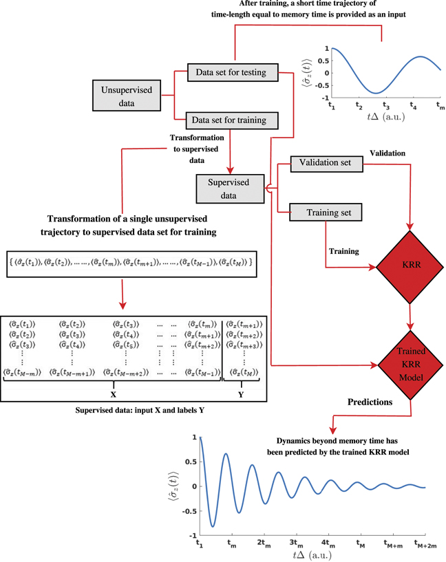
Figure 1. Flowchart of all steps during data preparation, training and predictions.
Download figure:
Standard image High-resolution imageFrom the data set of 1000 trajectories, 100 randomly chosen trajectories are taken as the hold-out test set, which we use for testing our approach and the results presented in this paper are shown for this hold-out set. With Δttrain = 0.1 and tm = 4, the remaining set of 900 unsupervised trajectories of time-length tM = 20 are transformed into 144 000 supervised trajectories of time-length tm = 4. The data set of supervised trajectories is randomly partitioned into two subsets: a training set, which contains 80% of the data and a validation set with 20% random trajectories of the set (see figure 1) for the optimization of hyperparameters σ and λ on the logarithmic grid [98]. For ML calculations we used the MLatom package [98–100] (training data and input files for MLatom can be found at https://doi.org/10.6084/m9. figshare.15134649 as described in data and code availability section). Since the cost of training a KRR model scales as N3, instead of training a single model, we reduced the training cost by training two separate models for symmetric and asymmetric cases, which halves the number of training points. The training for each case takes ≈8.20 h with parallel computation on 36 Intel(R) Xeon(R) Gold 6240 CPUs @ 2.60 GHz.
4. Results and discussion
After training our KRR model, it uses values taken with the step Δttrain from the short-time trajectory run with the HEOM up to the memory time tm as input vector x and predicts the value at the next time step tm+1. We prepare a new input vector by removing the first point and appending the value at tm+1 and predict with KRR the at the next time step tm+2. This process continues until trajectory reaches final run time. This way, KRR uses short-time HEOM trajectories run up to the memory time tm to predict long-time trajectories run up to time tM and beyond (see figure 1; the code, ML models, and necessary data for running dynamics with MLatom can be found at https://doi.org/10.6084/m9.figshare. 15134649 as described in data and code availability section; it is worth emphasising that the fed short-time input trajectories are unseen to our trained KRR models). This approach gives us the valuable information about the temporal evolution of the state population in contrast to alternative approaches, where ML was used to completely bypass HEOM dynamics and predict the final properties of interest such as transfer times and transfer efficiencies in the pigment–protein complexes [103].


Figure 2 shows results for symmetric SB model with a wide range of parameters. Similarly, figure 3 shows results for asymmetric SB model. Noteworthy, our KRR model can faithfully reproduce the reference HEOM trajectories at least up to run time 30 as we show in figures 2 and 3, which means that KRR is capable of extrapolating beyond the time-limit tM = 20 used for training. Figures 2 and 3 show small fraction of results. For the remaining results of the hold-out test set, interested readers are referred to the supporting information (https://stacks.iop.org/NJP/23/113019/mmedia). (In the supporting information, the trajectories are propagated up to tM = 20.) The predicted results cover a wide range of scenarios from strong environment to weak environment and from strong coupling to weak coupling. The errors for the hold-out test set of 100 trajectories are shown in table 1.

Figure 2. Expectation value of for symmetric SB model (i.e. = 0.0) as a function of time. Results predicted by KRR model (blue line) are compared to the HEOM results (red dots). The adopted parameters are: (a) λ = 0.2, ωc
= 8.0, β = 1.0; (b) λ = 0.4, ωc
= 10.0, β = 1.0; (c) λ = 0.2, ωc
= 10.0, β = 0.25; (d) λ = 0.1, ωc
= 4.0, β = 0.1; (e) λ = 0.8, ωc
= 3.0, β = 1.0; (f) λ = 1.0, ωc
= 2.0, β = 0.1. Here Δ = 1.0 and on x-axis t is multiplied by Δ, following reference [104]. All parameters are in atomic units.

Download figure:
Standard image High-resolution image
Figure 3. Expectation value of for asymmetric SB model (i.e. = 1.0) as a function of time. Results predicted by KRR model (blue line) are compared to the HEOM results (red dots). The adopted parameters are: (a) λ = 0.1, ωc
= 6.0, β = 0.75; (b) λ = 0.3, ωc
= 8.0, β = 1.0; (c) λ = 0.2, ωc
= 10.0, β = 0.25; (d) λ = 0.4, ωc
= 8.0, β = 0.75; (e) λ = 0.8, ωc
= 10.0, β = 1.0; (f) λ = 0.7, ωc
= 10.0, β = 0.1. Here Δ = 1.0 and on x-axis t is multiplied by Δ, following reference [104]. All parameters are in atomic units.

Download figure:
Standard image High-resolution imageTable 1. Mean absolute error (MAE), mean square error (MSE) and root mean square error for the hold-out test set of 100 trajectories within time-window 4–20.
| SB models | MAE | MSE | RMSE |
|---|---|---|---|
| Symmetric | 9.20 × 10⁻⁴ | 6.12 × 10⁻⁶ | 2.47 × 10⁻³ |
| Asymmetric | 1.97 × 10⁻³ | 8.00 × 10⁻⁵ | 8.94 × 10⁻³ |
From figure 2, we can see that the predictions by KRR model are very accurate for symmetric cases. For asymmetric SB model, the predicted result given in figure S3–(3f) of the supporting information slightly deviate from the exact HEOM results in the long-time regime. The possible reason is that the memory-time or in other words, the window-size of the base trajectory (|0 − tm |) is not enough for this case. In this work, we have considered the same memory time for both symmetric and asymmetric SB models, but it is advised to train separate models for symmetric and asymmetric SB cases with different memory times. The accuracy of the KRR model depends on memory time. By increasing the memory time, the KRR model gets more accurate in the predictions as shown for the hold-out trajectories in figure 4. The window-size of the base trajectory (|0 − tm |) should be wide enough, so that ML model can learn to differentiate among different trajectories. For not wide enough window-size, KRR model cannot differentiate well between two input trajectories, which results in a rapid deterioration of the accuracy.

Figure 4. MAE as a function of memory time tm . The MAE is averaged over 50 hold-out symmetric trajectories for the time-window t = 12–20.
Download figure:
Standard image High-resolution image
As predicted value is included in the input for the next time step, the error accumulation with time is inevitable, which imposes strict requirements on the accuracy of the predictions as for less accurate ML models the quality of trajectories will rapidly deteriorate. Figure S5 of supporting information shows the increase of absolute error in the predictions with the passage of time for the deviating trajectory figure S3–(3f) of supporting information. As KRR is a nonparametric ML model, the number of its regression coefficients increases with the increase of training points in contrast to parametric ML models, e.g. those based on neural networks, which fix the functional form and the number of parameters independently from the number of training points [105]. This makes the training of the KRR models very time consuming and requires large memory for huge training sets. To avoid this problem, we should keep the number of points in the training set as minimum as possible. It can be done by using farthest-point sampling [99], while choosing trajectories for training, or setting Δttrain to larger values while ensuring that it will not decrease the accuracy of the KRR predictions too much.
The computational cost-saving by our ML approach is substantial. The amount of time saving depends on the memory time and the trajectory time and in our case it is ca 90%. This reduction in computational time may allow longer simulations with HEOM model at low temperatures, where its cost and memory requirements increase very fast. In contrast, after training, the computational cost of our KRR model remains the same for all cases. On a single Intel(R) Core(TM) i7-10700 CPU @ 2.90 GHz, prediction of the whole trajectory beyond the initial memory time tm (up to 30 a.u.) takes ≈3 min. In the future, our approach can be combined with SEOM, which requires a large number of trajectories to have good convergence in the long-time regime. After generating short time trajectory of time-length tm with SEOM, our approach can be used to predict the long-time dynamics saving a tremendous amount of computational cost, which is currently the topic of our investigations.
5. Concluding Remarks
In this article, we have developed an ML approach to study quantum dissipative dynamics. We have demonstrated the ability of KRR to learn from relatively small amount of training data and predict the long-time quantum dissipative dynamics for two-level SB model without much loss of accuracy. After training, the KRR model requires short-time trajectory as input, and as an output it gives the dynamics for future times. The ability of predictions for future time makes KRR model or in general ML an appealing approach to avoid the calculation of expensive long-time dynamics. It can be combined with other approaches such as SEOM, which has bad convergence in long-time regime. Here, we have only demonstrated results for the two-level SB model, but our approach can be extended to multi-level systems given that the data for training is provided. In the end, with the establishment of the database with the dynamics data, the ML approach has great potential to become a useful low-cost computational tool for studying the quantum dissipative dynamics.
Acknowledgments
POD acknowledges funding by the National Natural Science Foundation of China (No. 22003051) and via the Lab project of the State Key Laboratory of Physical Chemistry of Solid Surfaces. The authors thank Alexei A. Kananenka for clarifying his approach.
Data availability statement
The data that support the findings of this study are openly available at the following URL/DOI: 10.6084/m9.figshare.15134649.
Supporting information
Additional plots for the test trajectories.
Author contributions
AU conceived the project, performed all the implementations, simulations, and analysis of the data, as well as written the original version of the manuscript. Both authors carried out the method development, discussed the results, and revised the manuscript. POD acquired funding for the project.
Data and code availability
The data and code are available at https://doi.org/10.6084/m9.figshare.15134649.