


Abstract
The Dyson series is an infinite sum of multi-dimensional time-ordered integrals, which serves as a formal representation of the quantum time-evolution operator in the interaction-picture. Using the mathematical tool of divided differences, we introduce an alternative representation for the series that is entirely free from both time ordering and integrals. In this new formalism, the Dyson expansion is given as a sum of efficiently-computable divided differences of the exponential function, considerably simplifying the calculation of the Dyson expansion terms, while also allowing for time-dependent perturbation calculations to be performed directly in the Schrödinger-picture. We showcase the utility of this novel representation by studying a number of use cases. We also discuss several immediate applications.
Export citation and abstract BibTeX RIS
1. Introduction
The Dyson series [1] is one of the fundamental results of quantum scattering theory. It is a perturbative expansion of the quantum time-evolution operator in the interaction-picture, wherein each summand is formally represented as a multi-dimensional integral over a time-ordered product of the interaction-picture Hamiltonian at different points in time. As such, the series serves as a pivotal tool for studying transition properties of time-dependent quantum many-body systems [2]. The Dyson series also has a close relation to Feynman diagrams in quantum field theory [3] and to the Magnus expansion in the theory of first-order homogeneous linear differential equation for linear operators [4].
Despite its fundamental role in quantum theory, one of the key challenges in using the Dyson series in practical applications remains the evaluation of the multi-dimensional integrals over products of time-ordered operators, making the calculation of the terms in the series an exceedingly complicated task [5]. In this paper, we derive an analytical, closed-form expression for the summands of the Dyson series, by explicitly evaluating the Dyson integrals. We accomplish this by utilizing the machinery of 'divided differences'—a mathematical tool normally used for computing tables of logarithms and trigonometric functions and for calculating the coefficients in the interpolation polynomial in the Newton form [6–12].
The main technical contribution of this work is an alternative, yet equivalent, formulation of the Dyson series wherein the summands are given in terms of efficiently computable divided differences of the exponential function. We argue that our novel representation, which is devoid of integrals and time ordering, makes it a very useful tool in the study of perturbation effects in many-body quantum systems—a fundamental branch of quantum physics.
In particular, this representation allows us to write an explicit, integral-free time-dependent perturbation expansion for the time-evolution operator in the Schrödinger-picture enabling us to carry perturbation calculations without the need to switch to the interaction-picture. To showcase the utility of our formulation, we work out a number of examples, for which we explicitly calculate the first few terms of the series. We begin by a brief introduction of divided differences, followed by the derivation of the integral-free representation of the Dyson series.
2. Divided differences—a brief overview
The divided differences [7, 8], which will be a major ingredient in the derivation detailed in what follows, is a recursive division process. The divided differences of a function f(⋅) is defined as

with respect to the list of real-valued input variables [x0, ..., xq ]. The above expression is ill-defined if some of the inputs have repeated values, in which case one must resort to the use of limits. For instance, in the case where x0 = x1 = ... = xq = x, the definition of divided differences reduces to:

where f(n)(⋅) stands for the nth derivative of f(⋅). Divided differences can alternatively be defined via the recursion relations

with i ∈ {0, ..., q − j}, j ∈ {1, ..., q} and the initial conditions

As is evident from the above, the divided differences of any given function f(⋅) with q inputs can be calculated with q(q − 1)/2 basic operations.
Divided differences obey the following properties: (i) linearity: for any two functions f(⋅) and g(⋅) and a number λ, the following holds. (f + g)[x0, ..., xq
] = f[x0, ..., xq
] + g[x0, ..., xq
] and (λ ⋅ f)[x0, ..., xq
] = λ ⋅ f[x0, ..., xq
]. (ii) Divided differences obey the Leibniz rule ![$(\enspace f\cdot g)[{x}_{0},\dots ,{x}_{q}]={\sum }_{k=0}^{q}\enspace f[{x}_{0},\dots ,{x}_{k}]\cdot g[{x}_{k},\dots ,{x}_{q}]$](https://content.cld.iop.org/journals/1367-2630/23/10/103035/revision2/njpac2daeieqn1.gif) . (iii) Invariance under permutation of inputs, namely, f[x0, ..., xq
] = f[xσ(0), ..., xσ(q)] where σ: {0, ..., q} → {0, ..., q} is a permutation. (iv) Any real-valued function f(⋅) obeys the mean-value theorem f[x0, ..., xq
] = f(q)(ξ)/q! where f(q)(⋅) stands for the qth derivative of f(⋅) and ξ is a number in the interval [min[x0, ..., xq
], max[x0, ..., xq
]].
. (iii) Invariance under permutation of inputs, namely, f[x0, ..., xq
] = f[xσ(0), ..., xσ(q)] where σ: {0, ..., q} → {0, ..., q} is a permutation. (iv) Any real-valued function f(⋅) obeys the mean-value theorem f[x0, ..., xq
] = f(q)(ξ)/q! where f(q)(⋅) stands for the qth derivative of f(⋅) and ξ is a number in the interval [min[x0, ..., xq
], max[x0, ..., xq
]].
In addition, a function of divided differences can be defined in terms of its Taylor expansion. For the special case of f(x) = e−itx , which will be of special importance in this study, we have

Moreover, it is easy to verify that
One may therefore write:
3. Divided differences formulation of the time-evolution operator
Usually, the go-to approach to tackling the dynamics of time-dependent systems is through the use of (time-dependent) perturbation theory in the interaction-picture [13, 14] where the Hamiltonian is written as

namely as a sum of a static (or 'free') Hamiltonian H0 (that is assumed to have a known spectrum) and an additional time-dependent Hamiltonian, V(t), that is treated as a perturbation to H0. The time-evolution operator in the interaction-picture is given by ![${U}_{I}(t)=\mathcal{T}\enspace \mathrm{exp}[-\mathrm{i}{\int }_{0}^{t}{H}_{I}(t)\mathrm{d}t]$](https://content.cld.iop.org/journals/1367-2630/23/10/103035/revision2/njpac2daeieqn2.gif) , a shorthand for the Dyson series
, a shorthand for the Dyson series

where  , and hereafter we use the q = 0 term to symbolize the identity operator.
The operator UI
(t) evolves the interaction-picture wave-function |ψI
(t)⟩ which is related to the Schrödinger-picture wave-function via  (in our units, ℏ = 1). Similarly, the Schrödinger-picture time-evolution operator U(t) is related to the interaction-picture operator via
  . In what follows we present an equivalent form for the Dyson series, equation (8), by systematically evaluating the integrals in the sum, writing V(t) as a sum of exponentials in t.
3.1. Generalized permutation operator representation of the perturbation Hamiltonian
We begin by denoting the eigenstates and eigenenergies of the free Hamiltonian H0 by  and
and  , respectively, such that H0|z⟩ = Ez
|z⟩. (For simplicity we assume a discrete countable set of eigenstates and eigenenergies). We will refer to
, respectively, such that H0|z⟩ = Ez
|z⟩. (For simplicity we assume a discrete countable set of eigenstates and eigenenergies). We will refer to  as the 'computational basis'. Next, we write the perturbation Hamiltonian V(t) as a sum of generalized permutation operators Πi
[15]:
as the 'computational basis'. Next, we write the perturbation Hamiltonian V(t) as a sum of generalized permutation operators Πi
[15]:

where every generalized permutation operator is further expressed as a product of a (time dependent) diagonal (in the computational basis) operator Di
and a bona-fide permutation operator Pi
. Specifically, the action of Di
and Pi
on a computational basis states is given by Di
|z⟩ = di
(z)|z⟩, where di
(z) is in general a complex number, and Pi
|z⟩ = |z'⟩ for some  depending on i and z. The i = 0 permutation operator will be reserved to the identity operator, that is,
  . Equipped with these notations, the action of a generalized permutation operator Πi
on a basis state |z⟩ is given by Di
Pi
|z⟩ = di
(z')|z'⟩, where z' depends on both the state z and the operator index i. We note that any Hamiltonian can be readily cast in the above form [11].
. Equipped with these notations, the action of a generalized permutation operator Πi
on a basis state |z⟩ is given by Di
Pi
|z⟩ = di
(z')|z'⟩, where z' depends on both the state z and the operator index i. We note that any Hamiltonian can be readily cast in the above form [11].
At this point, we write each diagonal operator, Di (t), in equation (9) as an exponential sum in t, that is,

where both  and
and  are (generally complex-valued) diagonal matrices and Ki
denotes the number of terms in the decomposition of Di
. (For more details as to how to carry out this decomposition efficiently, see references [16–18].) Thus, V(t) can be written as
are (generally complex-valued) diagonal matrices and Ki
denotes the number of terms in the decomposition of Di
. (For more details as to how to carry out this decomposition efficiently, see references [16–18].) Thus, V(t) can be written as

where, for simplicity, hereafter we fix Ki = K ∀ i, though this assumption can be easily removed. With this expansion of V(t), we can write the interaction-picture Hamiltonian HI (t) as

where we have defined  . Using this form of HI
(t) allows us to explicitly evaluate the time-ordered integrals of the Dyson series (8) (see appendix
. Using this form of HI
(t) allows us to explicitly evaluate the time-ordered integrals of the Dyson series (8) (see appendix
where we have defined the (time-dependent) coefficients

In addition, we have denoted iq
= (i1, i2, ..., iq
) and kq
= (k1, k2, ..., kq
) as multi-indices,  ,
,  with
with  and
and  for every j = 0, ..., q (remembering that the value of
  depends on that of z). The inputs for the divided-difference exponential are given by

for j = 0, ..., q − 1, where  and
and  (we have omitted the dependence of x0, ..., xq−1 on z, iq
and on kq
for a lighter notation). Importantly, the complex-valued
(we have omitted the dependence of x0, ..., xq−1 on z, iq
and on kq
for a lighter notation). Importantly, the complex-valued ![${\mathrm{e}}^{-\mathrm{i}t[{x}_{0},{x}_{1},\dots ,{x}_{q-1},0]}$](https://content.cld.iop.org/journals/1367-2630/23/10/103035/revision2/njpac2daeieqn21.gif) can be calculated efficiently, with computational complexity proportional to q2 (see reference [19] for additional details). Equation (13) is the main technical result of our paper. The equation is a reformulation of the Dyson series, equation (8), yet it includes only sums of efficiently-computable terms and is devoid of both integrals and time-ordering operators.
can be calculated efficiently, with computational complexity proportional to q2 (see reference [19] for additional details). Equation (13) is the main technical result of our paper. The equation is a reformulation of the Dyson series, equation (8), yet it includes only sums of efficiently-computable terms and is devoid of both integrals and time-ordering operators.
The current representation of UI (t) also allows us to obtain an integral-free time-dependent perturbation expansion of the Schrödinger-picture time-evolution operator U(t):

where

with  for j = 0, ..., q. We arrive at equation (17) by using identity 2 in appendix
Equation (16) allows us to explicitly carry out time-dependent perturbation calculations directly in the Schrödinger-picture without the need to invoke the interaction-picture.
4. Use cases
To showcase the immediate applicability of our approach, in what follows we illustrate, by examining a few examples, the utility of equation (16) in a variety of settings, specifically in scenarios where the time-ordered integrals of the Dyson series are cumbersome to calculate or lead to unnecessary complicated expressions.
Example 1. Transition amplitudes and Fermi's golden rule. Using the divided-differences series formulation of the time-evolution operator one may arrive at a rather simple expression for transition amplitudes, A(zin → zfin, t) = ⟨zfin|U(t)|zin⟩, between an initial eigenstate |zin⟩ and a final eigenstate |zfin⟩ of the free Hamiltonian H0 due to the perturbation effect of V(t), cf equation (7). Using equation (16) we find

where the second sum is over all multi-indices iq
that obey  .
.
Consider, for example, for the canonical, yet non trivial, case of the non-Hermitian Hamiltonian H = H0 + γF eiEt
where γ is a perturbation parameter and F a permutation matrix such that F|zin⟩ = |zfin⟩ and  . While the standard Dyson-series-based derivation of the transition amplitude beyond the first order expansion q = 1 (that is Fermi's golden rule) is cumbersome to derive and to calculate (see, e.g. references [20, 21]), the present formulation allows us to immediately write a succinct expression for transition amplitudes that are accurate to any order in γ. In particular, the qth order contribution for the transition amplitude is given very neatly by

for odd values of q, and can be calculated with O(q2) basic operations (for even values of q, A(q)(zin → zfin, t) = 0). The case q = 1 corresponds to Fermi's golden rule [22]. This simple expression showcases how the new formulation of the Dyson series can be used to explore properties of time-varying Hamiltonian systems that arise from perturbation orders that have not explored with prior methods.
Example 2.
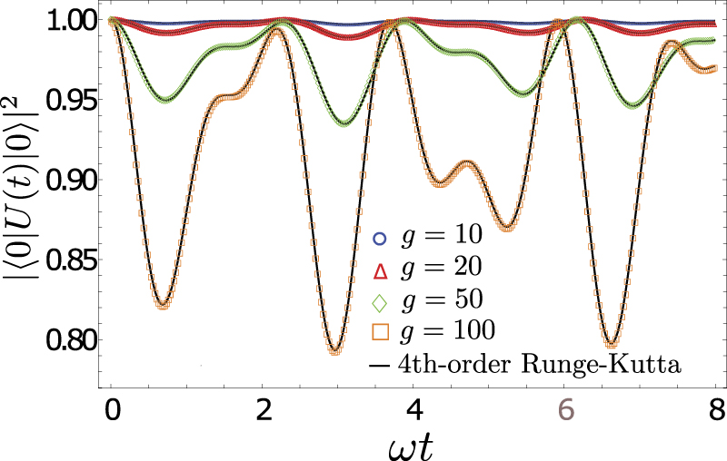
Time-oscillating two-level Hamiltonian system. To further illustrate the practical power of the integral-free description of the Dyson series and its ability to assist in uncovering new physics, we next consider the dynamics of two-level systems driven by highly oscillating time-dependent Hamiltonians of the form H = ω0
σz
+ gσx
cos ωt. Despite its apparent simplicity, calculating dynamical properties of this system still poses challenges to numerical integration methods whenever the driving oscillations are very fast, and it is an open problem that continues to be a very active area of research, for example in the study of evolution of qubits undergoing quantum gates [23] or in Bloch–Siegert systems, which play an important role in atomic physics [24] (it should be noted that in certain cases two-level systems admit analytical solutions in which case a numerical series expansion is not strictly necessary, see e.g. [25]). Our formulation on the other hand results in a compact description of the unitary operator (more information is given in appendix
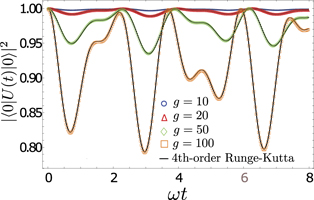
Figure 1. The probability to remain in the initial state |0⟩ (eigenstate of σz with eigenvalue + 1) for a highly oscillating (here, ω0 = 2ω = 200) two-level system for different values of time t. The figure shows numerically-exact calculations using the proposed method for a wide range of coupling strengths. The black lines passing through the data points correspond to numerically-exact solutions obtained using 4th-order Runge–Kutta simulations carried out independently to verify the correctness of the our results.
Download figure:
Standard image High-resolution imageExample 3. Time-oscillating infinite-dimensional Hamiltonian system. Next, we work out the expansion of the time-evolution operator for a particle moving under the influence of a harmonic potential perturbed by a periodic time-dependent anharmonic term, namely,

Identifying the static component as  , we rewrite the Hamiltonian in terms of the harmonic annihilation–creation operators (recall that ℏ = 1) as

To express V(t) in terms of generalized permutation operators, using the harmonic oscillator eigenstates {|n⟩} as the computational basis states, we rewrite the anharmonic operator  as
as  where Pi
= ∑n
|n + i⟩⟨n| and the matrix elements of the diagonal operators Di
are given by
where Pi
= ∑n
|n + i⟩⟨n| and the matrix elements of the diagonal operators Di
are given by
In terms of the above operators, the Hamiltonian can be written as

where  and
and  . Having cast the Hamiltonian in the appropriate form, it is straightforward to calculate the
  terms in the divided-differences expansion of U(t), as per equation (17). For example for q = 1 we obtain

where i1 ∈ {0, ±2, ±4}. Our formulation provides an easy way to compute the state of the system after time t. For an initial state |ψ(0)⟩ = |n⟩, we get the analytic closed-form expression  (see appendix
5. Summary and discussion
To conclude, in this work, we devised an alternative approach to time-dependent perturbation theory in quantum mechanics that allows one to readily calculate expansion terms. We derived an expansion that is equivalent to the usual Dyson series but which includes only sums of closed-form analytical simple-to-calculate expressions rather than the usual Dyson multi-dimensional time-ordered integrals. The terms at every expansion order in our new formulation coincide with those of the standard Dyson series, except that the Dyson integrals at every order replaced with finite sums. Therefore, both series share the same convergence criteria [27–30]. However, our new formalism allowed us to write an integral-free perturbation expansion for the time-evolution operator. We illustrated the utility of our approach by working out a number of use cases and calculated the series coefficients for a number of examples for which the usual Dyson series calculation is cumbersome, demonstrating the functionality and practicality of our approach.
Another area in which the divided-differences expansion can be applied, which we have not explored here, is quantum algorithms—algorithms designed to be executed on quantum computers. Specifically, the divided-differences expansion was recently shown to be a valuable tool in the derivation of quantum algorithm devised to simulate the time-evolution of quantum states evolving under time-independent [12] and time-dependent [31] Hamiltonians. There, it was shown that the divided-differences expansion allows for the time-evolution operator to be written as a sum of generalized permutation matrices, equivalently a linear combination of unitary (LCU) operators. As such, this representation of the time-evolution operator lends itself naturally to the quantum LCU lemma [32] which provides a prescription for efficiently simulating such operators on quantum circuits. We leave that for future work.
We believe that the formulation introduced here will prove itself to be a powerful tool in the study of time-dependent quantum many-body systems.
Acknowledgments
This work is supported by the US Department of Energy (DOE), Office of Science, Basic Energy Sciences (BES) under Award No. DE-SC0020280.
Data availability statement
The data generated and/or analysed during the current study are not publicly available for legal/ethical reasons but are available from the corresponding author on reasonable request.
Appendix A.: Derivation of an integral-free form for the Dyson series
Here, we derive the expression

Using the form of HI (t)

we can write the Dyson series for UI (t) as
where iq = (i1, i2, ..., iq ) and kq = (k1, k2, ..., kq ) are multi-indices. Acting with UI (t) on an arbitrary computational basis state |z⟩, we get
where we have defined  and
and  for every j = 0, ..., q (remembering that
  depends on z). Moreover, we define
  and similarly

with  . In addition, we have denoted
  and
and  . Following identity 1 in appendix B, the integrals appearing inside the parentheses in equation (A4) evaluate explicitly to the divided-differences exponential, that is,

with

(we have omitted the dependence of x0, ..., xq−1 on z, iq and on kq for a lighter notation). Using equation (A6), we can write the action of UI (t) on an arbitrary computational basis state in an integral-free form as

with the inputs to the divided-differences exponential given in equation (A7). We thus arrive at:

as claimed.
Appendix B.: Proofs of two identities of the exponent of divided-differences

where  . This identity is a variant of what is often known as the Hermite–Gennochi formula [8].
Proof. We start with the left-hand side of equation (B1). Making a change of variables tj = tsj we get

Next we prove by induction that

where  .
.
Base step (proving for q = 1): starting from the left-hand-side of equation (B3) we have

as required. In the first equality of equation (B4), we changed the integration variable ξ = s1 γ1, so that ξ ranges from 0 to γ1, and γ1 ds1 = dξ.
Hypothesis step: next, we assume the validity of equation (B3).
Induction step: based on this assumption, we now prove that

with  . Changing the integration variable s1 to ξ = γq+1
sq+1 + ⋯ + γ1
s1, so that ξ ranges from γq+1
sq+1 + ⋯ + γ2
s2 to γq+1
sq+1 + ⋯ + (γ2 + γ1)s2, and γ1 ds1 = dξ we get
. Changing the integration variable s1 to ξ = γq+1
sq+1 + ⋯ + γ1
s1, so that ξ ranges from γq+1
sq+1 + ⋯ + γ2
s2 to γq+1
sq+1 + ⋯ + (γ2 + γ1)s2, and γ1 ds1 = dξ we get
where from the induction assumption,

with  . Therefore, we obtain,
This concludes the proof.
Identity 2. Given an arbitrary multi-set of inputs {x0, ..., xq },

where x is an arbitrary constant and Δj = xj − x.
Proof. We prove equation (B9). By definition [8],

(assuming for now that all inputs are distinct). It follows then that

This result holds for arbitrarily close inputs and can be easily generalized to the case where inputs have repeated values, as claimed.
Appendix C.: Time-oscillating two-level Hamiltonian systems
Consider a time-dependent qubit system whose Hamiltonian has the form H = ω0
σz
+ gσx
cos ωt. We identify H0 = ω0
σz
(hence the computational basis is the Pauli-Z eigenbasis {|z⟩: z = 0, 1}) and V(t) = gσx
cos ωt. The time-dependent component V(t) contains a one permutation operators (M = 1), P1 = σx
, whose associated diagonal operators,  has two exponential terms (K = 2) such that
  with
with  . For reasons that would become clearer later we index the latter operators by k = ±1 (instead of k = 1, 2).
To write the time evolution operator, we first note that since there is only one off-diagonal operator in the Hamiltonian, there is also one sequence of off-diagonal operators per expansion order q, explicitly:

Moreover  , defined in equation (12) in the main text, is given by

with  for j = 0, ..., q, where
  and Σkj+1:q
is a shorthand notation to
and Σkj+1:q
is a shorthand notation to  . The last two equations define the time evolution operator of the system for any order expansion q, specifically,

where  .
.
Appendix D.: Time-oscillating infinite-dimensional Hamiltonian system
Below we provide additional calculations for the time-dependent anharmonic oscillator

discussed in the main text. Having computed the coefficients,  (see equation (19) in the main text), we may plot, as we do in figure 2(a), the population of every mode at various times. In the figure, the populations are given at t = 0.04 for ω = 1, Ω = 2, γ = 0.02 with the initial state |n = 4⟩ and an expansion cutoff of Q = 5. To ascertain the accuracy of the Dyson series truncated at different cutoff orders Q, we may also contrast the divided-differences expansion with exact-numerical results obtained via direct integration of the Schrödinger equation. In figure 2(b) we plot the infidelity 1 − |⟨ψ(t)|ψQ
(t)⟩|2 between the state |ψ(t)⟩, the solution of the time-dependent Schrödinger equation of this system, and the state as obtained by using divided-differences expansion for U(t), |ψQ
(t)⟩ = UQ
(t)|4⟩, that is, the state obtained by evolving |4⟩ under U(t) given by
(see equation (19) in the main text), we may plot, as we do in figure 2(a), the population of every mode at various times. In the figure, the populations are given at t = 0.04 for ω = 1, Ω = 2, γ = 0.02 with the initial state |n = 4⟩ and an expansion cutoff of Q = 5. To ascertain the accuracy of the Dyson series truncated at different cutoff orders Q, we may also contrast the divided-differences expansion with exact-numerical results obtained via direct integration of the Schrödinger equation. In figure 2(b) we plot the infidelity 1 − |⟨ψ(t)|ψQ
(t)⟩|2 between the state |ψ(t)⟩, the solution of the time-dependent Schrödinger equation of this system, and the state as obtained by using divided-differences expansion for U(t), |ψQ
(t)⟩ = UQ
(t)|4⟩, that is, the state obtained by evolving |4⟩ under U(t) given by

as a function of evolution time t.

Figure 2. (a) Probabilities of the various modes at t = 0.04 for the anharmonic Hamiltonian, equation (D1). Here, ω = 1, Ω = 2, γ = 0.02 and the initial state is |n = 4⟩. The blue circles are obtained from numerical integration of the Schrödinger equation while the orange triangles correspond to the divided-differences expansion up to order Q = 5. (b) Infidelity 1 − |⟨ψ(t)|ψQ (t)⟩|2 as a function of time. The various curves correspond to different truncation orders Q = 0, ..., 3. As we expect, the higher the expansion order is, the better the approximation becomes.
Download figure:
Standard image High-resolution image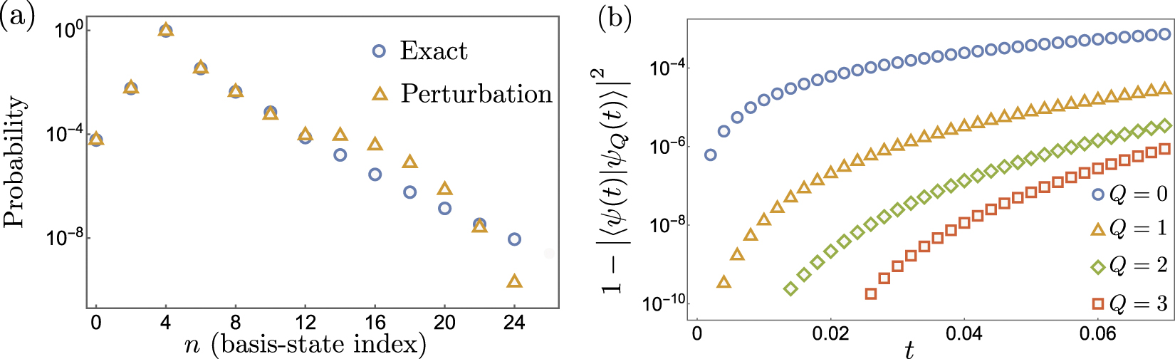