


Abstract
Using a test-particle model, we examine direct laser acceleration of electrons within a magnetic filament that has been shown to form inside a laser-irradiated plasma. We focus on ultra-high intensity interactions where the force of radiation friction caused by electron emission of electromagnetic radiation must be taken into account. It is shown that even relatively weak superluminosity of laser wave fronts—the feature that has been previously neglected—qualitatively changes the electron dynamics, leading to a so-called attractor effect. As a result of this effect, electrons with various initial energies reach roughly the same maximum energy and emit roughly the same power in the form of x-rays and gamma-rays. Our analysis implies that the primary cause of the superluminosity is the laser-heated plasma. The discovered strong interplay between superluminosity and radiation friction is of direct relevance to laser-plasma interactions at high-intensity multi-PW laser facilities.
Export citation and abstract BibTeX RIS

Original content from this work may be used under the terms of the Creative Commons Attribution 4.0 licence. Any further distribution of this work must maintain attribution to the author(s) and the title of the work, journal citation and DOI.
1. Introduction
Direct acceleration of plasma electrons by a high-intensity laser pulse [1–3] is a ubiquitous mechanism for energy transfer from the pulse to the irradiated plasma [4, 5]. It plays a key role in multiple applications utilizing ultra-intense laser technology [6], such as generation of energetic ion beams [7, 8] and generation of bright x-ray/gamma-ray beams [9–11]. The direct laser acceleration process in the presence of quasi-static plasma electric and magnetic fields remains an active area of research due to its complexity and it has been extensively studied using experiments [12–16], analytical theory [17, 18], and numerical simulations [1, 19, 20].
Construction of new multi-PW laser facilities like ELI-NP [21, 22], ELI beamlines [23], and CoReLS that are expected to reach peak intensities well in excess of 1022 W cm−2 [24] has generated additional interest in direct laser acceleration. At these intensities, accelerated electrons become efficient emitters of photons and the feedback from the resulting recoil must be self-consistently included into the description of electron dynamics [25]. The effect is commonly referred to as the radiation reaction or radiation friction, which is the term of choice in this manuscript (see [26] for a review of recent experimental and computational results). In two recent studies [27, 28], the authors examined the changes induced by the radiation friction on the direct laser acceleration process. The surprising and counter-intuitive finding is that the radiation friction can dramatically increase the electron energy gain from the laser pulse in the presence of a strong static azimuthal plasma magnetic field with a polarity that provides transverse electron confinement.
One feature of ultra-high intensity laser beams is that they are typically tightly focused to achieve the ultra-high laser intensity. Nevertheless, these beams are able to propagate through a plasma over distances that greatly exceed the vacuum Rayleigh length without significant diffraction (e.g. see [16] and references therein). Stable laser beam propagation can be further facilitated by introducing a structure in the form of a channel with a density that is lower than the density of the surrounding bulk plasma [9, 19]. Due to its limited transverse size and due to the presence of the plasma, the laser beam has a phase velocity vph that exceeds the speed of light c. It is convenient to introduce  that quantifies the relative degree of superluminosity. In general, δu depends on the characteristic transverse size R of the beam and on the electron plasma density ne. In recent fully self-consistent simulations for structured [19] and uniform targets [29], the relative superluminosity ranged from δu ≈ 6.6 × 10⁻³ to δu ≈ 2.9 × 10⁻².
It might appear that this level of superluminosity is sufficiently weak to be neglected. In fact, this was the approach in both of the studies mentioned earlier that focused on the role of the radiation friction while effectively considering luminal wave-fronts by setting vph = c [27, 28]. On the other hand, a separate study that has examined the impact of superluminosity, albeit in the absence of radiation friction, found that there exists a threshold for δu [17]. Above the threshold, the superluminosity can have a profound impact by enhancing the electron energy gain from the laser. The role of superluminosity in the presence of radiation friction and quasi-static plasma electric and magnetic fields is yet to be examined.
The purpose of this paper is to address this gap in knowledge by considering direct laser acceleration of electrons in a laser pulse with superluminal wave-fronts in the regime where the radiation friction has an appreciable effect on electron dynamics. We limit our analysis to the regime where the superluminosity is primarily caused by the presence of the plasma. We consider a magnetic filament with an azimuthal magnetic field sustained by a longitudinal plasma current. It has been shown using two- and three-dimensional kinetic simulations that such a configuration can be realized using laser-irradiated structured targets [9, 19, 30]. Our analysis is performed using a test-particle model with prescribed plasma and laser fields, including the magnitude of δu, which makes it easier to understand the interplay between the superluminosity and the radiation friction.
We find that even seemingly weak superluminosity (δu ≈ 10−2) that is typical for ultra-high intensity laser-plasma interactions [19, 29] can impact the dynamics of an electron experiencing radiation friction in a non-trivial way. In the luminal case, the maximum energy attained by an electron reduces over time due to the radiation friction. This then causes continuous reduction in the power of x-ray emission by the electron. We show that, in contrast to that, the maximum energy and the emitted power are nearly constant in the superluminal case following an initial transition period. Remarkably, the corresponding values are the same for a wide range of initial electron energies. We show that this feature is a manifestation of a so-called attractor behavior enabled by an interplay between the superluminosity and the radiation friction.
The rest of the manuscript is organized as follows. In section 2, we estimate the laser and target parameters that one needs to achieve the quasi-static magnetic filament configuration. In section 3, we provide estimates for the relative degree of superluminosity δu and show that its primary cause in the regime of interest is the presence of laser-heated plasma. In section 4, we formulate a simplified model for analyzing electron acceleration by an ultra-high intensity laser inside the magnetic filament. In section 5, we use the model to illustrate the key differences in electron dynamics caused by superluminosity in the absence of radiation friction. In section 6, we estimate this impact of radiation friction and show that there is a significant difference between the luminal (vph = c or δu = 0) and superluminal (vph > c or δu > 0) cases even at a relatively low level of superluminosity. In section 7, we examine long-term electron dynamics and show the existence of the so-called attractor behavior in the superluminal case. In section 8, we demonstrate that the attractor behavior makes the electrons into efficient emitters of radiation in the superluminal case. In section 9, we summarize our findings and discuss their implications.
2. Generation of laser-driven quasi-static magnetic fields (qualitative discussion)
In this paper, we explore electron dynamics for a specific configuration where an ultra-high intensity laser pulse drives a strong quasi-static azimuthal magnetic field while propagating through a plasma. This configuration is schematically show in figure 1. It has been observed in fully self-consistent 2D [9] and 3D [19] particle-in-cell (PIC) simulations, e.g. see figure 1 in [19] for detailed plots of fields and current density. In what follows, we estimate the laser and target parameters that one needs to achieve this configuration.
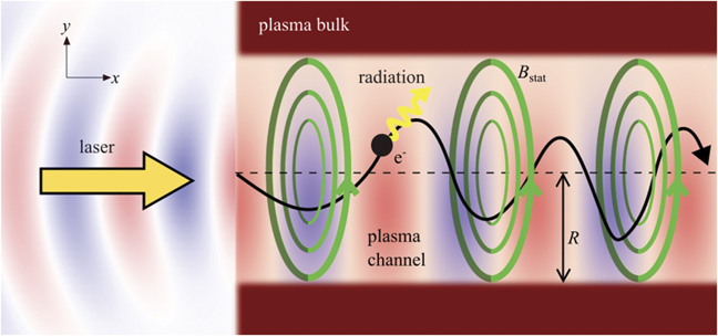
Figure 1. Electron acceleration in the presence of a laser-driven magnetic field Bstat (green) inside a laser-irradiated structured target (red) with a channel of radius R. The laser-accelerated electron whose trajectory is shown in black emits photons/radiation (yellow wavy arrow) in the forward direction due to its interaction with Bstat.
Download figure:
Standard image High-resolution imageThe configuration with a quasi-static magnetic field arises naturally if

where τe is the characteristic time of the electron response in the irradiated plasma and τL is the temporal duration of the laser beam. We can estimate the electron response time roughly as τe ≈ 2π/ωpe, where  is the electron plasma frequency that depends on the electron charge e, electron mass me, and the electron density ne. It is convenient to measure the electron density in the units of the classical critical density, nc, defined as the electron density that satisfies the condition
  , where ω is the carrier frequency of the laser pulse. We then have
  , where T ≡ 2π/ω is the period of laser oscillations. Equation (1) can now be re-written as a condition that relates the density in the target to the laser pulse parameters:
  .
.
The condition  provides a lower limit for the electron density to produce a quasi-static magnetic field. To ensure that a laser of a given intensity also propagates through the plasma, ne must remain significantly below the cutoff electron density n*. The condition that guarantees both the laser propagation and the slowly-varying magnetic field then reads

The cutoff density is equal to the critical density if the plasma electrons are non-relativistic. It however becomes dependent on the characteristic or average relativistic factor γav
if the plasma electrons are relativistic. The dependence on the γ-factor can be understood as an effective mass increase, since a relativistic electron roughly responds to electric and magnetic fields as a particle whose mass is γme rather than me. It can be shown that for a mono-energetic electric distribution n* = γnc for linear electromagnetic waves [31, 32]. We can thus approximately set n* ≈ γav
nc. The electron response time τe also becomes dependent on γav
if the electrons are heated to relativistic energy. Using the effective mass increase argument, we find that the original expression for τe must be multiplied by an additional factor of  . We thus conclude that equation (2), adjusted for the relativistic corrections in the cutoff density and the electron response time, reads

In the setup of interest, the electron heating to relativistic energy is caused by the laser beam itself. The resulting increase of the cutoff density is often referred to as the relativistically induced transparency [33]. The bulk of plasma electrons irradiated by the laser becomes relativistic when the normalized laser amplitude a0 that is approximately given by

is much greater than unity, i.e. a0 ≫ 1. Here I0 is the peak laser intensity and λ0 is the vacuum wavelength (note that λ0 = 2πc/ω). The characteristic relativistic factor γav can be approximated by γav ≈ (1 + a0/2). This expression describes well the values of γ observed in kinetic simulations with a0 ≫ 1 for a similar setup [34]. It should be used to assess the conditions given by equation (3) for a given a0.
In order to understand the implications of equation (3), we consider two different regimes relevant to two different laser systems: OMEGA EP with τL ≈ 1 ps, λ0 = 1.053 μm and ELI-NP with τL ≈ 27 fs, λ0 = 0.8 μm. In the case of OMEGA EP, we have  , where we took into account that λ0 = cT. It then follows from equation (3) that the desired regime can be reached using significantly sub-critical plasma densities, ne ≪ nc, and moderately relativistic laser amplitudes, a0 ∼ 1. Recently performed experiments at OMEGA EP with ne ∼ 10−2
nc and a0 ≈ 5 [16] are in the very same parameter space, so it is not surprising that 2D PIC simulations of the experiment have shown the presence of a strong slowly evolving plasma magnetic field [16]. In the case of ELI-NP, we have
, where we took into account that λ0 = cT. It then follows from equation (3) that the desired regime can be reached using significantly sub-critical plasma densities, ne ≪ nc, and moderately relativistic laser amplitudes, a0 ∼ 1. Recently performed experiments at OMEGA EP with ne ∼ 10−2
nc and a0 ≈ 5 [16] are in the very same parameter space, so it is not surprising that 2D PIC simulations of the experiment have shown the presence of a strong slowly evolving plasma magnetic field [16]. In the case of ELI-NP, we have  . The lower limit on ne is so much higher in this case that there is essentially no window in the significantly sub-critical density range. The slowly-evolving magnetic field can nevertheless be generated by a laser pulse with τL ≈ 27 fs, but this requires a much higher laser amplitude than in the previous example for OMEGA EP. For example, at a0 ≈ 200 we have a relatively wide window of ne according to equation (3), 100 ≫ ne/nc ≳ 1, but the suitable electrons densities are now in the classically near-critical range, ne ∼ nc, rather than in the significantly sub-critical range. The considered normalized amplitude of a0 ≈ 200 corresponds to a peak intensity of I0 ≈ 1023 W cm−2, which is, in fact, the projected peak intensity for ELI-NP. Recently published results of 3D PIC simulations with similar laser and plasma parameters [10] have confirmed that the considered laser pulse can indeed drive a strong slowly-evolving plasma magnetic field if the target density is sufficiently high.
It is worth pointing out that the propagation of an ultra-high intensity laser through a dense plasma can become unstable [9]. There are technical solutions for stabilizing the laser propagation while preserving the desired regime. One possible solution is to use a structured target that consists of a channel that has a lower electron density than that of the bulk [35]. If the channel density is ne/n* ≈ ne/γav nc ≪ 1 and the bulk density is ne/n* ≈ ne/γav nc ∼ 1, then the channel density fits the already discussed criterion while the channel walls provide optical guiding for the pulse. It must be stressed that the choice of densities does depend on the laser intensity because γav ≈ a0/2. Multiple simulation studies [9, 19, 30, 34, 36] have confirmed that such targets can indeed provide stable laser pulse propagation and, at the same time, generate slowly-evolving magnetic fields.
3. Estimates for the relative degree of superluminosity
The focus of this work is on the impact of superluminosity on direct laser acceleration of electrons, so here we provide estimates that can be used to assess the relative degree of superluminosity δu based on the target and laser parameters.
In our setup, the superluminosity has two causes: the presence of the laser-heated plasma and the finite width of the laser beam that is directly related to the width of the channel in the case of a structured target. We assume that the superluminosity is relatively weak, which is usually the case in the regimes of interest. The electron dynamics is sensitive to the difference between vph and c, so it is convenient to use

as a measure of the relative degree of superluminosity.
In order to estimate the impact of the laser-heated plasma, we consider a plane linear electromagnetic wave propagating through a uniform plasma with relativistic electrons. It is shown in [31] that the dispersion relation for the wave propagating across a plasma with two counter-streaming electron flows is

where k is the amplitude of the wave-vector and γ is the relativistic factor of the electrons in each of the streams (note that the laser propagates across rather than along the streams). It directly follows from this dispersion relation that

where we explicitly took into account that vph − c ≪ c to arrive to the expression on the right-hand side. Under the assumption that vph − c ≪ c, we can replace k2
c2 with ω2 on the right-hand side. In our case, the electron distribution is not mono-energetic, but the derived expression can still capture the essence of the electron response if we replace γ with the characteristic value γav
[32]. After taking into account that, by definition,  , we arrive to the following estimate

The propagation of the laser pulse is determined by the group velocity defined as vgr = ∂ω/∂k. It order to find vgr we take a derivative of equation (6) with respect to k, which yields ω∂ω/∂k = kc2. After using the definitions for vgr and vph, we find a well-known relation vgr = c2/vph. It follows from this relation that vgr is close to c for δu ≪ 1, with

In order to estimate the impact of the finite beam width, we consider a transverse magnetic (TM) mode propagating along a wave-guide of radius R with dielectric walls. We select the fundamental mode. It is shown using numerical simulations in [18] that the mode structure is similar to the analytical solution obtained by requiring the transverse electric field to vanish at the wall. The dispersion relation for the mode described by this analytical solution is

where Q ≈ 1.84. The structure of equation (10) is similar to that of equation (6). We can therefore obtain δu for this case by simply replacing ne/γav nc with Q2 c2/ω2 R2 in equation (8), which yields

We conclude this section by providing a relevant example for the discussion that will follow. We consider a laser pulse with a0 = 50 propagating through a channel whose radius is R = 5λ0. The channel is filled with a near-critical plasma, such that ne ≈ nc. We estimate the characteristic relativistic factor as γav ≈ a0/2. It then follows from equation (8) that the laser-heated plasma in our example can be expected to induce a relative degree of superluminosity roughly given by δu ≈ 2 × 10⁻². The superluminosity caused by the channel follows from equation (11), so we have δu ≈ 1.7 × 10⁻³ for the considered channel radius. Based on these estimates, we conclude that the superluminosity in the considered example is primarily caused by the laser-heated plasma. It is worth pointing out that the estimated value for δu is in the range of what has been observed in PIC simulations for high-intensity laser-plasma interactions [19, 29].
4. Test-electron model in the high-intensity regime
In this section, we formulate a simplified model that we later use to describe electron acceleration by an ultra-high intensity laser in the regime where the laser pulse generates a slowly-evolving magnetic field in the irradiated plasma.
We simplify the problem by considering a single electron, while treating the laser and plasma fields as given. In such a test-electron model, the electric and magnetic fields must be prescribed based on external knowledge. We use PIC simulations of laser propagation through a structured target, as the one discussed in [19], to inform our choice of the field structure. Based on the PIC simulation results of [19], we approximate the plasma magnetic field as a static field sustained by an electron current with a uniform current density jx = −|j0| directed along the axis of the laser beam propagation, which is the x-axis in our setup. It is convenient to introduce a dimensionless parameter,

which is the ratio of the electron current through a circle with radius λ0 to the non-relativistic Alfvén current JA = me c3/|e|. The static plasma magnetic field is azimuthal and it is given by

where

We approximate the laser beam by a plane electromagnetic wave with a superluminal phase velocity vph > c. As we show during our analysis, the plasma magnetic field limits the amplitude of transverse electron oscillations. We assume that the corresponding amplitude for the considered electron (see equation (31)) is smaller than the width of the laser beam and this gives the justification to neglect the transverse variation of the laser fields. In our model, the superluminal phase velocity is an input parameter. Particle tracking in PIC simulations [19] shows that the energetic electrons that the laser generates are injected into the laser beam transversely from the surrounding plasma. The implication of this is that these electrons do not typically experience a gradual rise in laser amplitude as would an electron that is initially located on the axis ahead of the laser pulse. We can thus make another simplifying assumption by setting the amplitude of the laser electric field, E0, to be constant. This simplification constrains the laser pulse duration (see section 9) and it also ignores laser depletion. Based on our assumptions and without any loss of generality, we represent the laser as a plane linearly polarized wave with


where

is the phase variable. The amplitude E0 can be expressed in terms of the normalized wave amplitude a0, previously defined in equation (4), using the relation a0 = |e|E0/me cω.
The relation between Bwave
and Ewave
that follows from equations (15) and (16), i.e. Bwave
= (c/vph)Ewave
, implies that the plasma contribution to the dispersion relation dominates over the contribution associated with the transverse nonuniformity of the field. As shown in appendix
In this paper, we are focused on scenarios where a0 ≫ 1, so we anticipate for the electron to experience violent acceleration and, as a result, to emit an appreciable amount of energy in the form of electromagnetic radiation. We account for the loss of energy associated with the emission through the so-called force of radiation friction. This force, f RF, is anti-parallel to the electron momentum p in the case of an ultra-relativistic electron [25], with

where  is the relativistic factor and re ≡ e2/me
c2 ≈ 2.8 × 10⁻¹⁵ m is the classical electron radius. Equation (18) has a form that is convenient for performing estimates because the product of the round brackets is dimensionless. Equation (18) implies that the energy of individual photons emitted by the electron is much smaller than the electron energy. This is indeed the case if the quantum nonlinearity parameter
is the relativistic factor and re ≡ e2/me
c2 ≈ 2.8 × 10⁻¹⁵ m is the classical electron radius. Equation (18) has a form that is convenient for performing estimates because the product of the round brackets is dimensionless. Equation (18) implies that the energy of individual photons emitted by the electron is much smaller than the electron energy. This is indeed the case if the quantum nonlinearity parameter

is small. Here Bcrit ≈ 4.4 × 10¹³ G is the magnetic equivalent of the well-known Schwinger (or critical) electric field [37]. The characteristic energy of emitted photons is  , so that
  is indeed much smaller than γme
c2 for χe ≪ 1. In the regimes considered in this paper, χe ⩽ 0.07 and the use of equation (18) is justified.
is indeed much smaller than γme
c2 for χe ≪ 1. In the regimes considered in this paper, χe ⩽ 0.07 and the use of equation (18) is justified.
The electron dynamics in our model is then described by the following equations:


where r and p are the electron position and momentum, t is the time, E = E wave is the total electric field, and B = B wave + B stat is the total magnetic field. In general, the electron trajectory in our configuration is three-dimensional and significant electron oscillations along the z-axis can potentially develop from small displacements in this direction [38]. Here we limit our analysis to flat electron trajectories in the (x, y)-plane with pz = 0. For such a trajectory, equations (20) and (21) reduce to


where


It can be shown that, in the absence of the radiation friction, equations (22) and (25) conserve the following dimensionless quantity [19]:

where we took into account that z = 0 for the considered trajectories. The conservation of S has been extensively used to analyze electron dynamics, e.g. it provides an upper limit on the amplitude of transverse displacements [29].
The force of radiation friction breaks this conservation law by changing the value of S during the electron motion. We readily find from equations (22)–(25) that the rate of change is

We note that vph enters the derived expression in such a way that we can expect it to influence not just the value of the rate but also its sign. In section 6 we show that this is indeed the case and that the superluminosity can profoundly alter the electron dynamics.
5. Energy gain in the absence of radiation friction
In this section, we illustrate the key differences in electron dynamics caused by superluminosity in the absence of radiation friction. A detailed analytical investigation of similar regimes where a radial electric field rather than an azimuthal magnetic field confines the electron is given in [17]. In the regimes considered here where the radiation friction is neglected, the dimensionless parameter S defined by equation (28) remains constant. The evolution of S due to radiation friction and its impact on electron dynamics are examined in sections 6 and 7.
All of the examples in this section use a0 = 50 and α = 15. This choice of α is informed by PIC simulations from [19] where a laser pulse with a normalized amplitude of a0 = 50 drives a longitudinal electron current corresponding to α ≈ 15 defined by equation (12). We consider an electron that is initially (t = 0) placed on axis (y = 0) with a transverse momentum  (note that px
= 0 and pz
= 0). This setup mimics the transverse injection of electrons into the laser pulse observed in PIC simulations [19]. To find the electron dynamics, we numerically solve equations (22)–(25) with the described initial conditions. It follows from equation (28), that, for the considered initial conditions (px
= pz
= 0 and y = 0), S is equal to the initial γ-factor denoted as γi
, which provides a helpful illustration of its meaning. Note that it remains constant during the electron motion due to the absence of the radiation friction.
(note that px
= 0 and pz
= 0). This setup mimics the transverse injection of electrons into the laser pulse observed in PIC simulations [19]. To find the electron dynamics, we numerically solve equations (22)–(25) with the described initial conditions. It follows from equation (28), that, for the considered initial conditions (px
= pz
= 0 and y = 0), S is equal to the initial γ-factor denoted as γi
, which provides a helpful illustration of its meaning. Note that it remains constant during the electron motion due to the absence of the radiation friction.
The electron gains energy from the transverse laser electric field Ey —the only electric field component in our model. The energy is first transferred from Ey to transverse electron oscillations and then it is redirected by the laser magnetic field Bz towards the forward-directed motion. The recipe for generating energetic electrons is to create the conditions where vy remains antiparallel to Ey over an extended period of time despite the oscillations of Ey at the electron location. These Ey oscillations are caused by the difference between vx < c and vph ⩾ c and they manifest the dephasing between the electron and the laser wave fronts.
The azimuthal magnetic field can create the conditions favorable for energy enhancement via transverse electron deflections. The effect of this is evident from figure 2(a) where the black markers show the maximum γ-factor attained by the electron (γmax) as a function of S for a reference luminal case without the magnetic field, i.e. δu = 0 and α = 0. The blue markers in the same plot show γmax for a luminal case with the magnetic field, i.e. δu = 0 and α = 15. In the absence of the magnetic field, the considered transverse electron injection with py = pi limits the maximum energy gain to γmax/a0 ≈ a0/γi due to strong dephasing between the electron and the laser wave fronts (see equation (4.12) in [39]). In the presence of the magnetic field, the energy gain from the laser is greatly enhanced at high values of S.
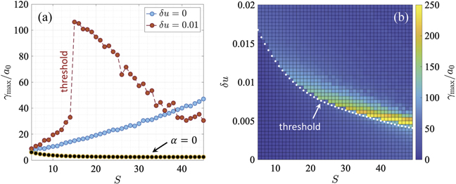
Figure 2. Maximum γ-factor, γmax, achieved by an electron from a laser with a0 = 50 while moving through a static azimuthal magnetic field sustained by a uniform current density that corresponds to α = 15. (a) Scan over S = γi for luminal (δu = 0) and superluminal (δu = 0.01) wave fronts. The black markers show a reference luminal case without the magnetic field, α = 0. (b) Scan over δu for S = γi between 5 and 50. Each marker in (a) and each square in (b) correspond to a time-interval of 3000T.
Download figure:
Standard image High-resolution imageThe energy enhancement occurs if the characteristic frequency of transverse electron oscillations, often called the betatron frequency, is comparable to the Doppler-shifted frequency of the laser. Both of these frequencies change as the electron energy increases. In the luminal case (δu = 0), the Doppler-shifted frequency decreases faster than the betatron frequency, which terminates the energy gain. In the superluminal case (δu > 0), the superluminosity increases the Doppler shifted frequency and, as a result, favorable acceleration conditions can be preserved even as the electron continues to gain energy. This idea was first put forward in [17], albeit for a different physical system.
The red markers in figure 2(a) show γmax for a laser with superluminal wave fronts, δu = 0.01. This data set is qualitatively different from that shown in blue and corresponding to the luminal case. In the superluminal case, γmax sharply jumps as S is increased from 14 to 15. At S ⩾ 15, the energy gain is greatly enhanced due to the superluminosity via the already explained mechanism. The observed threshold behavior was first derived in [17]. Figure 2(b) shows that the threshold value of S depends on the relative degree of superluminosity δu.
Figure 3 provides additional details regarding electron acceleration in the luminal and superluminal regimes shown in figure 2(a). In both cases, the electron has S = 17 and it is 'transversely injected', such that S = γi . The superluminosity maintains the conditions favorable for the prolonged energy gain while the laser electric field performs multiple oscillations, as seen in figure 3(d). In contrast to that, the electron is unable to continue gaining energy for even two Ey oscillations in the luminal case, as shown in figure 3(c). To quantify the rate of the energy gain, we plotted linear functions γfit = γfit(t) in figures 3(a) and (b). We have dγfit/dt ≈ 29.3/T in figure 3(a) and dγfit/dt ≈ 24.9/T in figure 3(b).

Figure 3. Electron energy gain in the luminal and superluminal cases in the absence of radiation friction for an electron with S = γi = 17. (a), (c), and (d) correspond to δu = 0; (b), (d), and (f) correspond to δu = 0.01. The yellow color marks the time intervals when the electron is gaining energy (vy Ey < 0). The dashed line in (a) is dγfit/dt ≈ 29.3/T and the dashed line in (b) is dγfit/dt ≈ 24.9/T.
Download figure:
Standard image High-resolution imageThe value of S, which is equal to γi in out setup, determines the amplitude of transverse electron displacements. It is convenient to re-write equation (28) as

where δu ⩾ 0 is a relative degree of superluminosity defined by equation (5). It follows from equation (30) that the maximum displacement is achieved in the limit of γ − px /me c → 0. We thus set px /me c ≈ γ and obtain that

It is appropriate to refer to the radial location with y = ±ymax as the magnetic boundary since the electron displacement is limited by the plasma magnetic field. An important takeaway from equation (31) is that the width of the magnetic boundary in the luminal case (δu = 0) increases with S. The superluminosity makes the location of the magnetic boundary energy-dependent—it expands with energy gain. The expansion of the magnetic boundary is evident from figure 3(d) where the amplitude of the transverse oscillation increases with γ. In contrast to that, no such expansion occurs in the luminal case shown in figure 3(c). The location of the magnetic boundary is an important quantity because (1) it determines whether or not the accelerated electrons can remain confined within a laser beam with a given width [29] and (2) it limits the amplitude of the plasma magnetic field Bstat sampled by the electron, which has a significant impact on the power of x-ray emissions (see section 8).
6. Estimates of the interplay between radiation friction and superluminosity
It is shown in section 5 that both the energy gain and the location of the magnetic boundary are determined by the value of S, which is a conserved quantity in the absence of radiation friction. The force of radiation friction changes the value of S. In what follows, we estimate this impact of radiation friction and show that there is a significant difference between the luminal (vph = c or δu = 0) and superluminal (vph > c or δu > 0) cases even at a relatively low level of superluminosity.
In order to motivate the analysis of this section, we have performed calculations for the luminal and superluminal cases with the same initial conditions as those used to obtain figure 3 in section 5, but with the radiation friction force now included into the equations of motion. The results are shown in figure 4 in blue. We find that the behavior of S is markedly different in these two cases. In the luminal case, seen in figure 4(c), S slowly decreases over time. In the superluminal case, seen in figure 4(d), S increases and roughly doubles in value during the energy gain. This change in S visibly impacts the maximum energy attained by the electron. Figure 5 provides additional information regarding the electron dynamics for these two cases to facilitate our analysis.

Figure 4. Electron dynamics with radiation friction (blue) and without the radiation friction (black) for luminal and superluminal cases. (a) and (c) correspond to δu = 0; (b) and (d) correspond to δu = 0.01. The electron starts its motion at t = 0 with S = 17. The black curves in (a) and (b) are the same as those in figures 3(a) and (b).
Download figure:
Standard image High-resolution image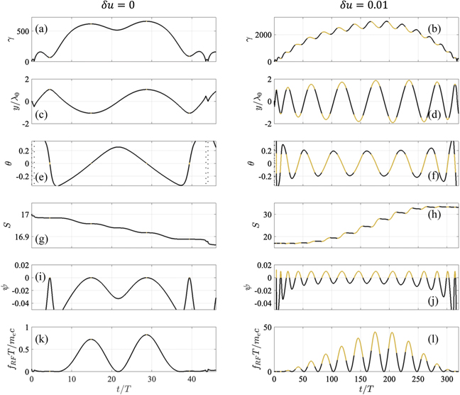
Figure 5. Electron dynamics for luminal ((a), (c), (e), (g), (i) and (k)) and superluminal ((b), (d), (f), (h), (j) and (l)) cases with δu = 0 and δu = 0.01 in the presence of radiation friction. In each case, the yellow segments correspond to ψ > 0. The electron starts its motion at t = 0 with S = γi = 17 in both cases. The curves for γ and S are the same as those shown in blue in figure 4.
Download figure:
Standard image High-resolution imageThe evolution of S is described by equation (29) that we now re-write as

where

The sign of dS/dt is determined by ψ, with dS/dt > 0 for ψ > 0 and dS/dt < 0 for ψ < 0. The rate of change however depends not only on ψ, but also on the amplitude of the radiation friction force | f RF|. The strength of this force, given by equation (18), increases with the relativistic factor γ. We thus assume the electron to be ultra-relativistic in our analysis. Otherwise, the change in S induced by the radiation friction is minimal.
We start by examining ψ and how its sign changes along the electron trajectory. The sign of ψ depends on the orientation of the electron momentum due to its explicit dependence on px . In the case of a transversely moving electron, i.e. px = 0, we have ψ < 0, so this type of motion reduces S. In the case of a laser-accelerated electron, the motion is never fully transverse during the energy gain process, as evident from figure 5(f) that shows

which is the angle between the electron momentum and the direction of the laser propagation. The absolute value of θ shown in figure 5(f) remains below 0.2 along most of the electron trajectory (see figure 5(d)). It is then appropriate to make an additional simplification by assuming that |θ| ≪ 1. We express ψ in terms of θ,

and set cos θ = 1 − θ2/2 to obtain the following approximate expression:

In the θ2-term, we replaced vph with c to take into account that the superluminosity is relatively weak in the regimes under our consideration.
In the luminal case, we have

along the majority of the electron trajectory. This expression needs to be corrected only for very small values of θ2 such as in the vicinity of the radial turning points. It follows form equation (36) that ψ becomes positive for

and it reaches its maximum value of  at θ = 0. This very narrow range of θ and the extremely small value of
  at ultra-relativistic electron energies suggest that ψ can effectively be treated as a negative function in the luminal case. The example shown in figure 5, where the yellow segments correspond to ψ > 0, confirms the validity of this approach (see figure 5(i) for the color-coded plot of ψ). An important implication of our finding is that S, whose time evolution is described by equation (32), decreases over time in the luminal case due to the radiation friction. Figure 5(g) further supports this conclusion.
At δu ≫ 1/2γ2, the superluminosity becomes a major factor in determining the values of ψ and the evolution of S. In this regime, equation (36) reduces to

The function ψ again reaches its maximum value at radial turning points, but this value is now much greater than in the luminal case:  . The transition between ψ < 0 and ψ > 0 occurs at

rather than at  . Since
  , the function ψ remains positive over a much wider range of angles, which translates into a much longer segment of the electron trajectory. For the superluminal case with δu = 0.01 shown in figure 5,
  , whereas max|θ| ≈ 0.2 along the majority of the trajectory (see figure 5(f) for θ as a function of time). As a result, ψ indeed remains positive along an appreciable part of the electron trajectory. It is also worth pointing out that the condition δu ≫ 1/2γ2 that ensures the dominance of the superluminosity is satisfied for γ ≫ 50 at δu = 0.01, which makes our analysis suitable for the majority of the energy gain process.
We have shown that the superluminosity makes ψ positive near radial turning points, which, in turn, causes S to increase while the electron is moving along the corresponding segments of the trajectory. The rate at which S changes over time depends on the amplitude of the radiation friction force. Near the radial turning points, the contributions from the laser electric and magnetic fields tend to compensate each other because the electron momentum is directed almost forward, i.e. |θ| ≪ 1. As a result, the radiation friction force is primarily determined by the plasma magnetic field Bstat, so we have

This expression follows from equation (18) after replacing B with B stat and setting E = 0 (this effectively accounts for the compensation of the effects from the laser electric and magnetic fields, as they are eliminated from the expression). Using equations (13) and (14), we find that

The turning point is located close to the magnetic boundary whose location, y = ±ymax, is given by equation (31). We set  to obtain the following expression:

We combine this estimate with the estimate for ψ near radial turning points,  , to obtain the following maximum rate of increase for S from equation (32):

where we set c/vph = 1 since the superluminosity is assumed to be weak.
Figures 5(l) and (h) that show | f RF| and S in the superluminal case with δu = 0.01 confirm our estimates. It follows from equation (43) that | f RF|T/me c ≈ 55 for γ = 3000 and S = 25, which is in good quantitative agreement with the exact result shown in figure 5(l). We find that S indeed increases near radial turning points and the rate of increase goes up with γ, as predicted by equation (44). The corresponding segments are shown in yellow in figure 5(h).
The sign of dS/dt changes as |θ| increases and exceeds  during electron motion from a radial turning point towards the axis. The net change in the value of S during one transverse oscillation is then determined by how much time the electron spends with
  , when S decreases, compared to the amount of time spent near turning points (
 ), when S increases. This observation allows us to conclude that by increasing the characteristic slope of its trajectory the electron can transition from a regime with a net gain in S to a regime with a net loss. In the next section, we use this observation to analyze long-term electron dynamics.
7. Long-term electron dynamics and attractor behavior
In section 6, we found that the radiation friction force can have opposite effects on the parameter S in the luminal and superluminal cases. In the absence of radiation friction, S is a constant of motion and strongly affects the energy attained by an accelerating electron. In this section, we examine how the changes in S induced by the radiation friction impact the electron energy gain.
7.1. Luminal case
We start by considering the luminal case. In general, the temporal profile of γ is a sequence of peaks similar to that shown in figure 5(a). The value of S changes during each peak, but this change is relatively slow on the time scale of a single peak (see figure 5(g) for the profile of S). This aspect simplifies our analysis, enabling us to treat the maximum energy attained during a single peak as if S were a constant. Figure 4(a) that compares the energy gain for constant and varying S further confirms that this is indeed reasonable. The evolution of the maximum energy attained by the electron can now be predicted from the scan shown in figure 2(a) and obtained in the absence of the radiation friction force. As the value of S gradually decreases, γmax/a0, shown with blue markers, should decrease as well.
Figure 6 shows the evolution of γ and S in the luminal case over 11 000 laser periods for an electron that starts its motion with S = 17. At the end of this time interval, we have S ≈ 7, as seen from the blue curve in figure 6(c). The height of peaks in figure 6(a) decreases as a result, which agrees with our prediction. Figure 6(d) shows ⟨γ⟩, which is the γ-factor averaged over 500 laser periods. This quantity decreases as well due to the reduction of S.
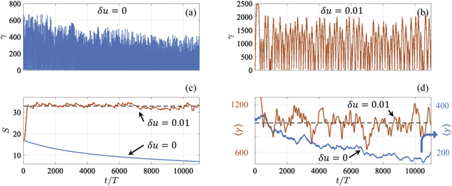
Figure 6. Evolution of γ ((a) and (b)) and S (c) in luminal and superluminal cases over 11 000 laser periods. The electron starts its motion at t = 0 with S = 17 in both cases. Panel (d) shows ⟨γ⟩, which is the γ-factor averaged over 500 laser periods, for the luminal and superluminal cases. The dashed line in (c) corresponds to S = 32.8. The dashed line in (d) corresponds to ⟨γ⟩ = 973.
Download figure:
Standard image High-resolution imageThe scan over the initial value of S shown in figure 7(a) confirms that the gradual reduction of S is a general trend for the luminal case. The reduction in S causes the maximum attainable γ-factor to decrease. Figure 7(c) shows the maximum γ-factor attained by the electron (denoted as γmax) after 1800 laser periods. The color-coding indicates the corresponding value of S. For reference, the black markers shows γmax without the radiation friction (note that this data set is similar to that shown with blue filled markers in figure 2(a)). The reduction in S is more pronounced at higher values of S. This is because the electron is able to reach higher values of γ in this cases, which enhances the amplitude of the radiation friction force that is responsible for the reduction of S.
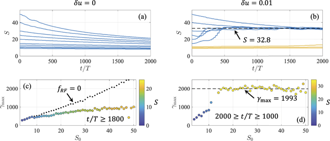
Figure 7. ((a) and (b)) The time evolution of S for luminal, δu = 0, and superluminal, δu = 0.01, cases. The dashed line in (b) is S = 32.8. The yellow curves in (b) correspond to S0 = 9, 10, and 11, where S0 is the value of S at t = 0. (c) The color-coded circles show the maximum γ attained by an electron at t/T ⩾ 1800 as a function of S0 in the luminal case, where the color indicates the value of S at the moment when γ reaches γmax. The solid black markers shows γmax over 2000 laser periods without the radiation friction. (d) The color-coded circles show the maximum γ attained by an electron at 2000 ⩾ t/T ⩾ 1000 as a function of S0 in the superluminal case, where the color indicates the value of S at the moment when γ reaches γmax. The dashed line is γmax = 1993.
Download figure:
Standard image High-resolution image7.2. Superluminal case
The approach used to examine the luminal case can be applied to examine the electron dynamics in a laser pulse with superluminal wave fronts. Without any loss of generality, we again consider the case of δu = 0.01.
Figure 6 shows in red the time evolution of S and γ over 11 000 laser periods for an electron that starts its acceleration with S = 17. In section 6, we examined the dynamics of this electron over the first 350 laser periods, which covers a single energy gain peak. Figure 6(c) shows that, after the initial increase, S stays around the horizontal dashed line that corresponds to S = 32.8. A similar patterns is true for the maximum γ-factor, with the only difference being that it experiences an early drop. The time-averaged γ-factor in figure 6(d) fluctuates around ⟨γ⟩ = 973 shown with a horizontal dashed line.
The observed reduction in γmax is consistent with the dependence of γmax on S in the absence of the radiation friction shown in figure 2(a). The initial value of S = 17 in the considered example is to the right of the discontinuity, so it is in the region where γmax decreases with the increase of S, which is the trend that we observe.
The value of S however stops increasing once it reaches the level of roughly S = 32.8. Rather than remaining constant, S performs fluctuations. In section 6 we showed that the sign of dS/dt is determined by the slope of the electron trajectory through function ψ. Therefore, the considered example suggests that it is possible for the contribution from trajectory regions with ψ > 0 to become on average balanced by the contribution from regions with ψ < 0 in the superluminal case.
A scan over the initial value of S shown in figure 7(b) reveals that S = Sa ≈ 32.8 acts as an attractor at the considered level of relative superluminosity (δu = 0.01). The blue curves correspond to S above the discontinuity for γmax in figure 2(a), whereas the yellow curves correspond to S below the discontinuity. The radiation friction is enhanced for S above the discontinuity because of a much higher γmax and this is what causes the rapid convergence to Sa for the blue curves. A closer look at electron trajectories shows that the characteristic slope of trajectories with S > Sa is steeper than the characteristic slope of trajectories with S < Sa . As a result, the electron with S > Sa spends more time moving along the segments with ψ < 0 that correspond to dS/dt < 0, which causes a net loss of S until it approaches Sa .
The discovered attractor behavior has a major impact on electron energy gain because the parameter S controls γmax attained by an electron. Figure 7(d) shows γmax after 1000 laser periods as a function of initial S, denoted as S0. The color indicates the current value of S at the time when γ = γmax. We find that both γmax and S are roughly the same for the electrons with S0 > 13. Therefore, γmax converges to roughly 2000 as a consequence of the attractor behavior that causes S to converge towards Sa . This result is in stark contrast to the behavior observed in the luminal case and it demonstrates the strong interplay between the superluminosity and the radiation friction.
8. Impact of superluminosity on x-ray emission
We have so far discussed the impact of the superluminosity on electron energy gain under the influence of the radiation friction force. The considered electrons emit x-rays and gamma-rays during their motion, so the changes in the energy gain should necessarily lead to changes in the photon emission. In this section, we show that the attractor behavior discovered in section 7 makes the electrons into efficient emitters of radiation in the superluminal case.
We find the time-evolution of the electron energy by multiplying equation (20) by v , which yields

The second term on the right-hand side is the energy lost per unit time by the electron due to the radiation friction. Therefore, the power of photon emission due to the radiation friction is given by

where we have taken into account that, according to equation (18), f RF is anti-parallel to v .
As shown in the two examples from figure 5, the amplitude of the radiation friction force peaks at radial turning points. The underlying cause is the increase of the plasma magnetic field, Bstat, with the radius. The amplitude of f RF near radial turning points was estimated in section 6 and it is given by equation (41). We use this expression and take into account that the emitting electrons are ultra-relativistic, p ≈ γme c, to find that near radial turning points we have

which means that  . It is more convenient to express this scaling in terms of the amplitude of the transverse electron displacement, y = ±ymax. In order to do this, we use the explicit dependence of Bstat on y given by equation (42), which yields

The main result of our estimates is the scaling  of the radiated power with the amplitude of the transverse displacements and the relativistic factor γ.
Figure 8(a) shows PRF over 500 laser periods for an electron that starts its motion with S = 30. The power of the emission is considerably higher in the superluminal case (δu = 0.01) after 200 laser periods. The underlying cause is the derived scaling for PRF. In the luminal case, the value of S decreases over time, which causes the maximum γ-factor attained by the electron to decrease and the magnetic boundary located at y = ±ymax to shrink (see equation (31)). These two aspects are shown in figure 8(b), where the magnetic boundary calculated using equation (31) is shown with solid black curves above and below the axis. Both aspects contribute to the reduction of PRF, as predicted by equation (48). In the superluminal case, the value of S experiences a modest increase due to the attractor behavior discussed in section 7. The key feature here is that there is no continuous reduction of S, so the electron is able to regularly achieve γmax ≈ 2000 predicted by figure 7(d). Moreover, as the γ-factor increases during the acceleration process, the magnetic boundary inflates due to the superluminosity. This trend is predicted by equation (31) and it is clearly visible in figure 8(c). The much higher γ-factor and the wider magnetic boundary at later times lead to a much higher PRF in the superluminal case than in the luminal case.
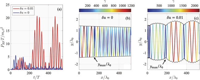
Figure 8. (a) Photon emission power in luminal and superluminal cases over 500 laser periods for an electron that starts its motion at t = 0 with S = 30. ((b) and (c)) The corresponding electron trajectories. The color shows the electron γ-factor. The solid black lines show the magnetic boundary, y = ±ymax, calculated according to equation (31).
Download figure:
Standard image High-resolution imageIn order to confirm that the two considered examples present a general trend, we have performed a scan over the initial value of S, denoted as S0. We are particularly interested in the emission at later times, such that the attractor behavior has enough time to manifest itself. Figure 9 shows ⟨PRF⟩, which is the emission power averaged over 500 laser periods for 2000 ⩾ t/T ⩾ 1500. In agreement with the already discussed examples, ⟨PRF⟩ is roughly an order of magnitude higher in the superluminal case (δu = 0.01) than in the luminal case (δu = 0). At S0 ⩾ 14, ⟨PRF⟩ in the superluminal case fluctuates around ⟨PRF⟩ ≈ 2.36me c2/T, shown with a horizontal dashed line. The near-constant level of ⟨PRF⟩ is a manifestation of the attractor behavior (illustrated in figure 7) that causes γmax to become essentially independent of S0 above S0 ⩾ 14 at t > 1000T. The spike at S0 = 13 is a transient feature associated with the transition from S0 to Sa ≈ 33 during the time-averaging interval. The maximum γ spikes, as predicted by figure 2(a), which, in turn, enhances the emission compared to the emission of the electrons whose S had converged to Sa ≈ 33 prior to the time-averaging.

Figure 9. Time-averaged radiated power in luminal (δu = 0) and superluminal (δu = 0.01) cases as a function of S0, where S0 is the value of S at t = 0. The averaging is performed over 500 laser periods for 2000 ⩾ t/T ⩾ 1500. The square markers show the power in the luminal case multiplied by a factor of 10 in order to improve the visibility of the data-set. The horizontal dashed line is ⟨PRF⟩ ≈ 2.36me c2/T.
Download figure:
Standard image High-resolution imageOur key finding is that, on average, the laser accelerated electrons emit with near-constant power due to the interplay between the superluminosity and the radiation friction. In contrast to that, the emitted power continuously decreases in the luminal case due to shrinkage of the magnetic boundary caused by the radiation friction. Therefore, the superluminosity has the ability to turn electrons into efficient emitters of radiation.
9. Summary and discussion
We have examined direct laser acceleration of electrons within a magnetic filament sustained by a uniform longitudinal plasma current. The laser intensity and the plasma density must satisfy the condition given by equation (3) for this configuration to exist. Our focus is on the regime of ultra-high intensity (a0 = 50) where the force of radiation friction caused by electron emission of electromagnetic radiation must be taken into account. We found that there is a strong interplay between this force and the superluminosity—the feature that has been previously ignored or overlooked.
We have compared two cases: a luminal case with δu = 0 and a superluminal case with δu = 0.01 (vph = 1.01c). It should be noted that a similar degree of superluminosity has been observed in simulations for tightly focused high-intensity laser pulses [29]. In the luminal case, the maximum energy attained by an electron reduces over time due to the radiation friction. This then causes a continuous reduction in the power of x-ray emission by the electron. In the superluminal case, the maximum energy and the emitted power are nearly constant following an initial transition period. Remarkably, the corresponding values are the same for a wide range of initial electron energies. We have shown that this feature is a manifestation of the attractor effect enabled by the interplay between the superluminosity and the radiation friction.
The discovered attractor effect relies on the radiation friction and it therefore requires ultra-high laser intensities to present itself. This regime is well within current capabilities of multiple laser facilities [6], since our results with a0 = 50 correspond to a peak intensity of 5 × 10²¹ W cm−2. The maximum amplitude of the radiation friction in our case roughly scales as  . It is thus possible that the regime can be extended to lower intensities by optimizing the magnetic field accessed by the electrons and the maximum energies they achieve.
The fact that the maximum amplitude of the radiation friction depends on γBstat rather than on a0 is a distinctive feature of the considered regime that must be accounted for when evaluating the photon emission. We have  , so χe also peaks at radial turning points. The maximum value of the quantum nonlinearity parameter χe can then be estimated as
  , where
  is the plasma magnetic field at the magnetic boundary |y| = ymax defined by equation (31). The photon emission near the radial turning points must be treated as a quantum process if the value of χe exceeds 0.1 due to the increase of γ and/or
  . One possible algorithm for accomplishing this is described in [40]. This algorithm was used in [27] for a setup similar to the one considered here. It remains to be seen whether or not the switch to the quantum emission qualitatively changes the conclusions regarding the attractor behavior.
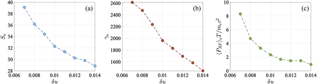
In order to examine the impact of δu, we have performed a scan shown in figure 10. We varied δu between 0.007 and 0.014, which roughly covers the range where we have the threshold associated with the superluminosity in figure 2(b). Our scan shows that γmax and ⟨PRF⟩ increase at lower values of δu for the electrons with S ≈ Sa. This behavior can be understood using figure 2(b) that shows an increase in γmax above the threshold at lower δu. We found that the range of the initial values of S impacted by the attractor effect shrinks at lower values of δu. Again, this can be understood using the scan shown in figure 2(b). According to our analysis of section 7, the attractor value Sa is above the threshold. As the threshold moves to higher values of S, the window of available S shrinks.
Figure 10. The attractor effect as a function of the relative superluminosity δu = (vph − c)/c. Sa is the attractor value of the parameter S. γa is the value of γmax for the electrons with S ≈ Sa.  is the time-averaged emitted power by the electrons with S ≈ Sa.
Download figure:
Standard image High-resolution image
As shown in section 3, δu is a potentially adjustable parameter. We have considered a regime where δu is primarily determined by the electron density, so the adjustment can then be achieved by changing ne inside the channel, with δu ≈ ne/a0 nc. Low density foams (ne ∼ nc), as those used in [14], can be employed to explore the electron dynamics for δu close to 10−2 (as in figure 10) at a0 > 50. The dependence for δu provided by equation (8), i.e. δu ≈ ne/a0 nc, should be interpreted as a scaling relation only. No numerical coefficient is given, as our estimates are not sufficiently accurate to determine such a coefficient. One should use at least 2D and preferably 3D PIC simulations to determine δu [19, 29] for given laser and target parameters. It must be pointed out that the presented analysis must be modified if, for a given target geometry, δu is primarily determined by the channel radius. The changes would affect the relation between Ewave and Bwave (see equations (15) and (16)). Additionally, the longitudinal laser electric field related to the radial field nonuniformity should be included into the model in this regime.
In this work, we have exclusively used the test-particle model, which enabled us to clearly identify the attractor effect. The model is however limited to a single particle, so one has to use a fully self-consistent approach (e.g. a 2D PIC simulation) that can describe the electron injection in order to predict the electron spectrum. However, the test-particle model developed here can serve as an essential tool for selecting and narrowing down the parameter range in scans involving PIC simulations. One of these parameters is the width of the laser beam or, equivalently, the channel radius, since the two are usually matched for better coupling [9]. It has to be less than the width of the magnetic boundary set by ymax. For the parameters used to generate figure 8(c), the radius of the channel and thus the laser beam has to be at least 3λ0. Otherwise, the electrons will be lost before gaining their maximum energy.
The test-particle model also provides constraints on the required propagation length by the laser pulse and the laser pulse duration. The attractor behavior in figure 7(b) manifest itself by t ≈ 500T. The electrons are ultra-relativistic, so the corresponding travel distance with the laser is then roughly 500 μm. The accelerating electrons can also outrun the laser pulse during their acceleration, because the longitudinal velocity vx
is likely to exceed the group velocity vgr. In order to estimate, the required pulse duration, we take into account that, according to equation (9), vgr − c ≈ − cδu. This means that the electron slip with respect to the laser wave-fronts is roughly equal to the distance by which the ultra-relativistic electron advances forward relative to the laser pulse. In figure 5(b), the phase slip for the shown time duration is Δ /2π ≈ 9. This means that the laser pulse has to be longer than 9λ0 or, equivalently, longer than 30 fs for λ0 = 1 μm.
In order to make preliminary predictions based on our results, we note that in a PIC simulation the electrons are injected with a wide range of S values. Recall that the initial value of S corresponds to the initial γ-factor, γi , of the transversely injected electrons. One typically finds that S = γi < a0. We can then conclude that, as the window of initial S values influenced by the attractor effect shrinks, the number of participating electrons can be expected to decrease. In order to maximize the number of participating electrons, one should aim to increase δu. On the other hand, δu needs to be reduced if the goal is to maximize the electron energy gain, as indicated by the scan shown in figure 10(b). Finally, we note that the upper limit on S can be increased by increasing the laser intensity, so a0 can serve as an additional control knob when exploring the described attractor effect.
Acknowledgments
This material is based upon work supported by the Department of Energy National Nuclear Security Administration through the National Laser Users' Facility (NLUF) under Award No. DE-NA0003944; by the Department of Energy National Nuclear Security Administration under Award No. DE-NA0003856; by the University of Rochester, and by the New York State Energy Research and Development Authority.
Data availability statement
The data that support the findings of this study are available upon reasonable request from the authors.
Appendix A.: Field structure of a TM mode in a dielectric wave-guide
We are considering a linear TM mode in a two-dimensional dielectric wave-guide whose geometry is similar to that shown in figure 1. The TM mode has two electric field components, Ex and Ey , and a single magnetic field component, Bz . We assume that the fields depend on x, y, and t only, with the dependence on x and t given by exp(ikx − iωt). The field structure is described by the following two vector equation:


where ɛ is the dielectric constant for the material inside the wave-guide. There are only three non-trivial equations for the considered mode:


It follows from equation (A.4) that there is a general relation between the transverse electric and magnetic fields:

The plane wave limit is obtained by setting ∂/∂y = 0. It follows from equation (A.3) that Ex = 0, which, as expected, means that there is no longitudinal field in a plane wave. Equations (A.4) and (A.5) yield the following dispersion relation:

We use this relation to eliminate ɛ from equation (A.6), which yields the following relation between the transverse electric and magnetic fields in a plane wave:
